Complex reaction noise in a molecular quasispecies model

Abstract

We have derived exact Langevin equations for a model of quasispecies dynamics. The inherent multiplicative reaction noise is complex and its statistical properties are specified completely. The numerical simulation of the complex Langevin equations is carried out using the Cholesky decomposition for the noise covariance matrix. This internal noise, which is due to diffusion-limited reactions, produces unavoidable spatio-temporal density fluctuations about the mean field value. In two dimensions, this noise strictly vanishes only in the perfectly mixed limit, a situation difficult to attain in practice.

, ,

1 Introduction

The study of replicator models of prebiotic evolution has received considerable theoretical attention during the past three decades [1]. There is a renewed and active interest in this subject owing to the crucial fact that the dynamics of real viral populations is known to be described by quasispecies [2, 3, 4]. To date, the bulk of the theoretical work devoted to the analysis of quasispecies dynamics has tacitly assumed spatially homogeneous conditions [1, 2, 3, 4, 5]. The importance of diffusive forces has begun to be recognized and taken into account [6, 7], but rather less attention, if any, has been payed to the presence of the unavoidable internal density fluctuations [8] that are necessarily present in all realistic incompletely mixed and diffusing systems of reacting agents [9]. In the deterministic approach to chemical and molecular species that diffuse and react, the fluctuations are simply ignored. Nevertheless, it is well known that if the spatial dimensionality $d$ of the system is smaller than a certain upper critical dimension $d_{c}$, the intrinsic fluctuations do play a decisive role in the asymptotic late time behavior of decay rates, and the results obtained from the mean field equations are not correct [10]. Even far from asymptotia, these fluctuations can strongly affect the dynamics on local spatial and temporal scales [11]. The mean field limit is strictly valid only in the infinite diffusion limit, because the reactions themselves induce local microscopic density fluctuations that can be amplified by the underlying nonlinear dynamics. This internal noise is multiplicative, and scales as the square root of the product of concentrations, with the consequence that the noise does not necessarily vanish in the large particle-number limit.

Given the relevance of molecular replicator models such as the quasispecies for viral dynamics and the key role played by fluctuations in nonlinear systems, this Letter has a twofold objective. First, we outline a rigorous derivation of the exact stochastic partial differential equations (SPDE) that govern the dynamics of a simple quasispecies model (denotes in this work a system comprised of a master plus mutant molecular species in competition for limited resources). Second, we study the nature of the internal fluctuations on the replicator evolution. But in order to achieve this latter goal, we must also develop and apply a method suitable for simulating multi-component SPDE’s with complex noise [12]. The validity of this approach is confirmed by numerical simulation. Neither of these objectives has been achieved before. We illustrate this method with a simple model that is analytically tractable, but the technique given here can be applied to more realistic chemical and molecular reaction processes.

2 Model

We consider a molecular quasispecies model with error introduced via the faulty self-replication of the master copy into a mutant species. The mutant species or, error-tail, undergoes non-catalyzed self-reproduction, but has no effect on the master species. The system is closed, only energy can be exchanged with the surroundings, where activated monomers react to build up self-replicative units. These energy rich monomers are regenerated from the by-product of the reactions by means of a recycle mechanism (driven by an external source of energy) maintaining the system out of equilibrium. The closure of the system directly imposes a selection pressure on the population. In what follows, ${M}^{*},I,I_{e}$ denote the concentrations of the activated energy rich monomers, the master and the mutant copies, respectively. The kinetic constants are introduced in the following reaction scheme.

Accurate replication with rate $AQ$:

$$\textrm{M}^{*}+\textrm{I}\stackrel{{\scriptstyle AQ}}{{\longrightarrow}}2\textrm{I}.$$ (1)

Error replication with rate $A(1-Q)$:

$$\textrm{M}^{*}+\textrm{I}\stackrel{{\scriptstyle A(1-Q)}}{{\longrightarrow}}\textrm{I}+\textrm{I}_{e}.$$ (2)

Mutant-species replication with rate $A_{e}$:

$$\textrm{M}^{*}+\textrm{I}_{e}\stackrel{{\scriptstyle A_{e}}}{{\longrightarrow}}2\textrm{I}_{e}.$$ (3)

Degradation of the master and mutant copies into monomers with rates $r,r_{e}$, respectively:

$$\textrm{I}\stackrel{{\scriptstyle r}}{{\longrightarrow}}\textrm{M},\qquad\textrm{I}_{e}\stackrel{{\scriptstyle r_{e}}}{{\longrightarrow}}\textrm{M}.$$ (4)

Re-activation of energy-depleted monomers (induced by a generic energy-driven reaction):

$$\textrm{M}\stackrel{{\scriptstyle energy}}{{\longrightarrow}}\textrm{M}^{*}.$$ (5)

The quality factor $Q\in[0,1]$. In order to keep the following development mathematically manageable, we will assume that the monomer reactivation step Eq.(5) proceeds sufficiently rapidly, so that we can in effect, regard the decay of $I$ and $I_{e}$, Eq.(4), plus the subsequent reactivation $\textrm{M}\stackrel{{\scriptstyle energy}}{{\longrightarrow}}\textrm{M}^{*}$ as occurring in one single step, i.e.,

$$\textrm{I}\stackrel{{\scriptstyle r}}{{\longrightarrow}}\textrm{M}\stackrel{{\scriptstyle energy}}{{\longrightarrow}}\textrm{M}^{*} \Rightarrow \textrm{I}\stackrel{{\scriptstyle r^{\prime}}}{{\longrightarrow}}\textrm{M}^{*}$$ (6)

$$\textrm{I}_{e}\stackrel{{\scriptstyle r_{e}}}{{\longrightarrow}}\textrm{M}\stackrel{{\scriptstyle energy}}{{\longrightarrow}}\textrm{M}^{*} \Rightarrow \textrm{I}_{e}\stackrel{{\scriptstyle r^{\prime}_{e}}}{{\longrightarrow}}\textrm{M}^{*}.$$ (7)

Here, $r^{\prime}$, $r_{e}^{\prime}$ are correspondingly, the combined effective decay plus regeneration rates of $I,I_{e}$ to the reactivated monomers $M^{*}$, although in what follows, we will simply write $r$ and $r_{e}$. This means that our continuum field theory, will depend on three $(M^{*},I,I_{e})$, instead of four $(M,M^{*},I,I_{e})$ concentration field variables. If we suppose the system is being bathed continuously by an external energy source, the monomer reactivation Eq.(5) is occurring continuously, and this should be a reasonable approximation. To complete the specification of the model, we allow for spatial diffusion. This is incorporated into the master equation associated with the above reaction scheme. The diffusion constants are denoted by $D_{s},D_{I}$ and $D_{e}$ for $M,I$ and $I_{e}$, respectively. The constraint of constant total particle number is automatically satisfied by the continuous chemical concentration fields in the mean-field limit. Most importantly, this provides a selection pressure on the quasispecies.

3 Complex Langevin equations

It is straightforward to write down the continuous time master equation corresponding to the above reaction scheme Eqs. (1,2,3,6,7). This master equation is then mapped to a second-quantized description following Doi [13]. From Doi’s operator language, we then pass to a path integral representation in terms of continuous stochastic fields [14] to obtain the following action $S$ valid for any space dimension $d$ (D. Hochberg, M.-P. Zorzano and F. Morán, unpublished notes):

$$S = \int dtd^{d}x\,\Big{(}\tilde{a}\big{(}\partial_{t}a-D_{s}\nabla^{2}a+Aab+A_{e}ac-rb-r_{e}c\big{)}$$ (8)

$$+ \tilde{b}\big{(}\partial_{t}b-D_{I}\nabla^{2}b-AQab+rb\big{)}$$

$$+ \tilde{c}\big{(}\partial_{t}c-D_{e}\nabla^{2}c-A(1-Q)ab-A_{e}ac+r_{e}c\big{)}$$

$$- AQab\big{(}{\tilde{b}}^{2}-\tilde{a}\tilde{b}\big{)}-A(1-Q)ab\big{(}\tilde{b}\tilde{c}-\tilde{a}\tilde{b}\big{)}-A_{e}ac\big{(}{\tilde{c}}^{2}-\tilde{a}\tilde{c}\big{)}\Big{)}.$$

In the mean field limit the continuous field variables $a,b,c$ in Eq.(8) correspond to the physical densities of the molecules $M,I,I_{e}$, respectively. The fields $\tilde{a},\tilde{b},\tilde{c}$, are conjugate to the internal fluctuations. Only if this noise is real, do $a,b,c$ continue to represent the physical densities. Otherwise, for imaginary or complex noise, these fields will likewise be imaginary or complex, but their stochastic averages $\langle a\rangle,\langle b\rangle$ , and $\langle c\rangle$ do however correspond to the real physical densities [15].

Since the $\tilde{a},\tilde{b},\tilde{c}$ fields appear quadratically in $S$, we can make use of the Hubbard-Stratanovich transformation to integrate over them exactly in the path integral $\int\mathcal{D}a\mathcal{D}{\tilde{a}}\mathcal{D}b\mathcal{D}{\tilde{b}}\mathcal{D}c\mathcal{D}{\tilde{c}}\,e^{-S[a,\tilde{a},b,\tilde{b},c,\tilde{c}]}$. This final step yields a product of delta-functional constraints which directly imply a set of exact coupled stochastic partial differential equations with specific noise properties (see below).

In particular, in a two-dimensional space and making the reasonable assumption that both master and mutant species diffuse equally $D_{Ie}=D_{I}=D$ and have equal effective degradation plus reactivation rates, i.e. $r_{e}/r=1$, the reaction-diffusion system in dimensionless variables is given as follows:

$$\frac{\partial\bar{a}}{\partial\tau} = (D_{s}/D)\nabla^{2}\bar{a}-\bar{a}\bar{b}-\bar{a}\bar{c}+\bar{b}+\frac{1}{\delta}\bar{c}+\hat{\eta}_{a}$$

$$\frac{\partial\bar{b}}{\partial\tau} = \nabla^{2}\bar{b}+Q\bar{a}\bar{b}-\bar{b}+\hat{\eta}_{b}$$

$$\frac{\partial\bar{c}}{\partial\tau} = \nabla^{2}\bar{c}+\delta(1-Q)\bar{a}\bar{b}+\delta\bar{a}\bar{c}-\bar{c}+\hat{\eta}_{c},$$

where $\nabla^{2}=\frac{\partial^{2}}{\partial\hat{x}^{2}}+\frac{\partial^{2}}{\partial\hat{y}^{2}}$ and $\vec{{\eta}}=(\hat{\eta}_{b},\hat{\eta}_{c},\hat{\eta}_{a})$ is the noise with $\langle\vec{{\eta}}\rangle=0$ and correlation matrix $B=\langle\vec{{\eta}}\vec{{\eta}}^{\prime T}\rangle$:

$$B(\hat{x},\hat{y};\tau)=\left(\begin{array}[]{ccc}\epsilon Q\bar{a}\bar{b}&\frac{1}{2}\epsilon\delta(1-Q)\bar{a}\bar{b}&-\frac{1}{2}\epsilon\bar{a}\bar{b}\\ \frac{1}{2}\epsilon\delta(1-Q)\bar{a}\bar{b}&\epsilon\delta^{2}\bar{a}\bar{c}&-\frac{1}{2}\epsilon\delta\bar{a}\bar{c}\\ -\frac{1}{2}\epsilon\bar{a}\bar{b}&-\frac{1}{2}\epsilon\delta\bar{a}\bar{c}&0\end{array}\right).$$ (12)

The initial condition $\bar{a}_{0},\bar{b}_{0},\bar{c}_{0}$ and the ratio of replication rates $\delta=A_{e}/A<1$ defines the scaled number of particles in the closed system $\bar{N}=\int\int d\hat{x}d\hat{y}(\bar{a}_{0}+\bar{b}_{0}+\frac{\bar{c}_{0}}{\delta})$. In the two-dimensional case the total number of particles is given by the ratio $N=\bar{N}/\epsilon$ where $\epsilon=A/D_{I}$ is the ratio of the reaction to the diffusion processes (in any dimension $d$, we have $\epsilon=(r/D_{I})^{d/2}A/r$). In the absence of noise $\vec{{\eta}}$ this reaction-diffusion system has a set of homogeneous solutions: (i) $\bar{b}=\bar{c}=0,\ \bar{a}=\bar{N}$, (the trivial solution); (ii) $\bar{b}=0,\ \bar{c}/\delta=\bar{N}-\frac{1}{\delta},\ \bar{a}=\frac{1}{\delta}$, if $\delta>1/\bar{N}$ and $\delta\leq Q$; and (iii) $\bar{c}/\delta=\frac{(\bar{N}Q-1)(1-Q)}{Q(1-\delta)},\ \bar{b}=\frac{(\bar{N}Q-1)(Q-\delta)}{Q(1-\delta)}$, $\bar{a}=1/Q$ if $Q>\delta$ and $Q>1/\bar{N}$. We want to understand how this deterministic, mean-field homogeneous solution, is modified by the internal multiplicative noise term with defined spatio-temporally varying covariance (the fields vary in both space and time). From inspection of the covariance matrix $B$ we see that this noise is proportional to $\epsilon$, the ratio between the reaction and diffusion processes. In the limit $\epsilon\rightarrow 0$ (infinite diffusion, i.e., a perfectly homogeneous system) there are no fluctuations, and we recover the mean field result. The noise term vanishes when $\bar{b}(\hat{x},t)=\bar{c}(\hat{x},t)=0$ (the trivial solution is an inactive state) and/or when $\bar{a}(\hat{x},t)=0$. If the system stays close to the mean field result, then $\bar{a}=1/Q$ and $\bar{b}$ and $\bar{c}$ scale as $(\bar{N}Q-1)$. Therefore the noise covariance is expected to scale with $\epsilon\bar{N}$. Our main interest here is the limit when the stochastic term makes a significant contribution $\epsilon\bar{N}=\epsilon^{2}N>1$. In this regime the problem can not be analyzed by perturbation theory and thus must be treated numerically .

Note that $B$ is a symmetric matrix with $\det B=-\frac{Q}{4}\bar{a}^{3}\bar{b}\bar{c}\epsilon^{3}\delta^{2}(\bar{b}+\bar{c})$, i.e. it is negative definite. Thus it either has one or three negative eigenvalues, suggesting that at least one noise component will have negative auto-correlation, and will therefore be imaginary. We expect this situation to be relatively common in reaction-diffusion systems with multiple species.

4 Results

We next apply the Cholesky decomposition, which is used when the symmetric matrix is positive definite, to relate this correlated noise to an uncorrelated one. We apply this algorithm for the first time here to a case with negative definite correlation matrix to obtain the “square root” $L$, where some of the terms are manifestly imaginary. This is very useful for relating the noise $\vec{\eta}$ to a new real white Gaussian noise $\vec{\xi}$ with $\langle\vec{\xi}\vec{\xi}^{\prime T}\rangle=1$, such that $\vec{\eta}=L\vec{\xi}$ :

$$\hat{\eta_{b}}= \sqrt{\epsilon\bar{a}} \sqrt{Q\bar{b}}\xi_{1},\qquad\hat{\eta_{c}}=\sqrt{\epsilon\bar{a}}\left(\frac{\delta(1-Q)\sqrt{\bar{b}}}{2\sqrt{Q}}\xi_{1}+\frac{\delta\sqrt{4Q\bar{c}-(1-Q)^{2}\bar{b}}}{2\sqrt{Q}}\xi_{2}\right),$$

$$\hat{\eta_{a}}= \sqrt{\epsilon\bar{a}} \left(-\frac{\sqrt{b}}{2\sqrt{Q}}\xi_{1}+\frac{1}{2\sqrt{Q}}\frac{(1-Q)\bar{b}-2Q\bar{c}}{\sqrt{4Q\bar{c}-(1-Q)^{2}\bar{b}}}\xi_{2}\right)$$

$$+ \sqrt{\epsilon\bar{a}} \frac{\sqrt{-1}\sqrt{Q}\sqrt{\bar{b}\bar{c}+\bar{c}^{2}}}{\sqrt{4Q\bar{c}-(1-Q)^{2}\bar{b}}}\xi_{3}.$$ (13)

This transformation allows us to separate the real and imaginary parts of the noise, a extremely useful feature to have for setting up and running a stable numerical simulation.

The noise $\hat{\eta_{a}}$ for the nutrient field $\bar{a}$, Eq.(4), always has an imaginary component and since all the equations are coupled to the nutrient $\bar{a}$, even if the initial condition for $\bar{a},\bar{b},\bar{c}$ is real, the fields will, in principle, have both real and imaginary parts, and thus we have to solve a system of 6 partial differential equations, one for each field ($\Re\bar{a},\Im\bar{a},\Re\bar{b},\Im\bar{b},\Re\bar{c},\Im\bar{c}$) with two-dimensional diffusion and noise. We expect the imaginary fields to be zero in the average, since the stochastic averages $\langle a\rangle,\langle b\rangle$ , and $\langle c\rangle$ correspond to the physical densities [15].

Integrating the system numerically we confirmed that the scaled number of particles was conserved and remained real $\Re\bar{N}=\bar{N}$, and $\Im\bar{N}=0$ (within computational errors) . We found that, independently of the initial condition and noise intensity, it always converged to the same state with spatial fluctuations around this value: $\langle\frac{\bar{c}}{\delta}\rangle_{\hat{x},\hat{y}}=\frac{(\bar{N}Q-1)(1-Q)}{Q(1-\delta)},\ \langle\bar{b}\rangle_{\hat{x},\hat{y}}=\frac{(\bar{N}Q-1)(Q-\delta)}{Q(1-\delta)}$, $\langle\bar{a}\rangle_{\hat{x},\hat{y}}=1/Q$, which is the mean-field solution An example of these spatial fluctuations is shown in Fig. (1) at $\tau=25$ for $\epsilon=1$ and $N=\bar{N}=10^{3}$, with $D_{s}/D=10$, $Q=0.92$, and $\delta=0.8$. In the case of $\bar{b}$ and $\bar{c}$, the densities show spatial fluctuations of up to $+1\%$ (in white) and $-1\%$ (in black) with respect to the mean field value. Inspection of the figure clearly shows that the master copy and mutant species are spatially anti-correlated. In the case of $\bar{a}$, the fluctuations range in the order of $\pm 5\%$ about the mean field value $\bar{a}=1/Q$.

$\bar{a}(\hat{x},\hat{y},\tau=25)$	$\bar{b}(\hat{x},\hat{y},\tau=25)$	$\bar{c}(\hat{x},\hat{y},\tau=25)$

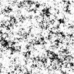
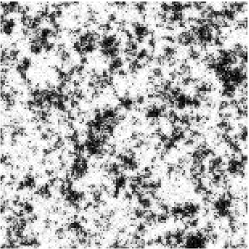
Figure 1: Long-time spatial distribution of the fields when $Q=0.92,\delta=0.8,D_{s}/D=10$ and $\epsilon=1$, $N=\bar{N}=10^{3}$. The three fields show fluctuations greater than $1\%$ about the mean-field value.

Next we explore the dependence of the spatio-temporal field fluctuations $\sigma^{2}_{\bar{b}(\tau)}=\langle(\bar{b}(\tau)-\langle\bar{b}(\tau)\rangle_{\hat{x},\hat{y}})^{2}\rangle_{\hat{x},\hat{y}}$ etc., in $\epsilon$ and $N$. In Fig. 2-left we show the deviation $\sigma_{\bar{b}(\tau)}$ scaled by $\sqrt{N}\epsilon$ for $N=\frac{\bar{N}}{\epsilon}=10^{3}$ and two different cases of $\epsilon$. As expected, $\sigma_{\bar{b}}$ scales with $\sqrt{N}\epsilon$, in this case as $0.04\times\sqrt{N}\epsilon$. Next we show the same for $N=10^{4}$, the mean value of $\sigma_{\bar{b}}$ is the same but the deviations with respect to it (which is related to the kurtosis of the distribution) increase with $N$. Notice that the relative weight of these fluctuations with respect to the mean-field value decreases with the number of particles since $\bar{b}\propto\bar{N}$ and therefore $\sigma_{\bar{b}}/\bar{b}\propto 0.04\sqrt{N}\epsilon/(N\epsilon)\propto 0.04/\sqrt{N}$.

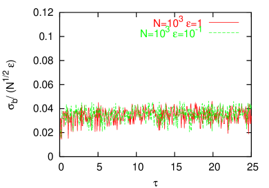
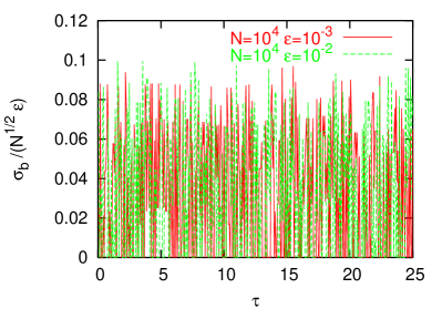
Figure 2: Time evolution of the fluctuations $\sigma_{\bar{b}(\tau)}=\sqrt{\langle(\bar{b}(\tau)-\langle\bar{b}(\tau)\rangle)^{2}\rangle}$ scaled by $\sqrt{N}\epsilon=\sqrt{\bar{N}\epsilon}$ for $N=10^{3}$ (left) and $N=10^{4}$ (right) with $\epsilon$ between $10^{-3}$ and $1$. The fluctuations around the mean-field value increase with $N$ and $\epsilon$.

5 Conclusions

Deriving the Langevin equation description from the Master equation provides a quick analytic survey of the global system dynamics (stationary states, etc), as well as the strength and characteristics of the internal noise and its dependence on the spatial dimensionality. For any dimension, the system can be solved numerically with high accuracy. This is in contrast to the direct Monte Carlo simulation of the system, such as in [16], where no preliminary analytic information can be given on the effects of reaction noise or dimensionality dependence. We have shown that the local deviations with respect to the mean-field solution scale with the number of particles and the ratio between the reaction and diffusion processes. The fluctuations vanish only in the perfectly mixed limit, when the diffusion processes are infinitely fast ($\epsilon=0$). Thus, even in the case of very high diffusion rates, an autocatalytic system can show important deviations with respect to the perfect mixing limit, provided that the number of particles in the reactor system is sufficiently high. For systems with a higher degree of non-linearity (i.e., third-order), these deviations may eventually lead the system to new asymptotic states and also induce the formation of spatial patterns [8]. Regarding the error catastrophe, this concept differs from virology to molecular replicator dynamics. In the former, the error catastrophe implies the proliferation of lethal mutations with the subsequent loss of viral infectivity, and consequently, the extinction of the viral population. This is reflected in our model as the trivial solution (i). On the other hand, solution (ii) corresponds to the error catastrophe state predicted by molecular replicator dynamics where there is no wild type population, while there is an error tail. We have found that this solution is an absorbing barrier. Finally, spatial diffusion and internal noise must in fact play an important role in the correct description of viral infection dynamics, where typically, bottlenecks of different intensities may lead to infection of host cells by limited numbers of viral particles [17].

We thank Carlos Escudero for many useful discussions and for working through some preliminary analytic calculations and Esteban Domingo for reading the manuscript and suggesting additional references. M.-P.Z. is supported by an INTA fellowship. The research of D.H. is supported in part by funds from CSIC and INTA and F.M. by grant BMC2003-06957 from MEC (Spain).

References

- [1] M. Eigen and P. Schuster, The Hypercycle–A Principle of Natural Self-Organization, Springer, Berlin, 1979.
- [2] E. Domingo, C.K. Biebricher, M. Eigen and J.J. Holland, Quasispecies and RNA Viruses: Principles and Consequences, Eureka.com, Austin, 2001.
- [3] C. Biebricher and M. Eigen, Virus Research 107 (2005) 117.
- [4] C.K. Biebricher and M. Eigen, Current Topics in Microbiol. Immunol. 299 (2006) 1.
- [5] M.A. Andrade, J.C. Nuño, F. Morán, F. Montero and G.J. Mpitsos, Physica D 63 (1993) 21.
- [6] P. Chacón and J.C. Nuño, Physica D 81 (1995) 398.
- [7] M.B. Cronhjort and C. Blomberg, Physica D 101 (1997) 289.
- [8] D. Hochberg, M.-P. Zorzano and F. Morán, J. Chem. Phys. 122 (2005) 214701.
- [9] I.R. Epstein, Nature 374 (1995) 321.
- [10] K. Kang and S. Redner, Phys. Rev. Lett. 52 (1984) 955.
- [11] M.P. Zorzano, D. Hochberg and F. Morán, Physica A 334 (2004) 67.
- [12] An imaginary noise Langevin equation without diffusion has been treated in O. Deloubrière, L. Frachebourg, H.J. Hilhorst and K. Kitahara, Physica A 308 (2002) 135.
- [13] M. Doi, J. Phys. A: Math. Gen. 9 (1976) 1465.
- [14] L. Peliti, J. Physique 46 (1985) 1469.
- [15] M.J. Howard and U.C. Täuber, J. Phys. A:Math. Gen. 30 (1997) 7721.
- [16] S. Altmeyer and J.S. McCaskill, Phys. Rev. Lett. 86 (2001) 5819.
- [17] C. Escarmís, E. Lázaro and S.C. Manrubia, Current Topics in Microbiol. Immunol. 299 (2006) 141.