Stochastic Model of Yeast Cell Cycle Network

Abstract

Biological functions in living cells are controlled by protein interaction and genetic networks. These molecular networks should be dynamically stable against various fluctuations which are inevitable in the living world. In this paper, we propose and study a stochastic model for the network regulating the cell cycle of the budding yeast. The stochasticity in the model is controlled by a temperature-like parameter $\beta$. Our simulation results show that both the biological stationary state and the biological pathway are stable for a wide range of “temperature”. There is, however, a sharp transition-like behavior at $\beta_{c}$, below which the dynamics is dominated by noise. We also define a pseudo energy landscape for the system in which the biological pathway can be seen as a deep valley.

1 Introduction

Quantitative understanding of biological systems and functions from their components and interactions presents a challenge as well as an opportunity for interested scientists of various disciplines. Recently, a considerable amount of attention has been paid to the quantitative modeling and understanding of the budding yeast cell cycle regulation [1, 2, 3, 4, 5, 6, 7, 8, 9, 10]. In particular, Li et al. [3] introduced a deterministic Boolean network model and investigated its dynamic and structural properties. Their main results are that the network is both dynamically and structurally stable. The biological stationary state is a global attractor of the dynamics; the biological pathway is a globally attracting dynamic trajectory. These properties are largely preserved with respect to small structural perturbations to the network, e.g. adding or deleting links. However, one crucial point left unaddressed in their study is the effect of stochasticity or noise, which inevitably exists in a cell and may play important roles [11]. In this paper, we advance a probabilistic Boolean network [12, 13] on the protein interaction network of yeast cell cycle. We found that both the biological stationary state and the biological pathway are well preserved under a wide range of noise level. When the noise is larger than a value of the order of the interaction strength, the network dynamics quickly becomes noise dominating and loses its biological meaning.

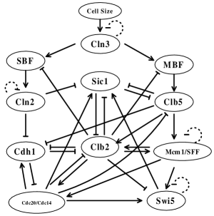
Figure 1: The cell-cycle network of the budding yeast. Each node represents a protein or a protein complex. Arrows are positive regulation, “T”-lines are negative regulation, dotted “T”-loops are degradation.

2 Method

Our stochastic model is based on the updated protein interaction network of Li et al. [3], which is depicted in Fig. 1. Nodes in the figure represent proteins or protein complexes. Arrows represent positive interaction, or “activation”. Lines with a bar at the end represent negative interaction, or “repression”. Dotted loops with a bar represent self-degradation. We refer the reader to Ref. [3] for a full biological account of this network. Here we only give a very brief summary. There are four phases in the cell cycle process: the G1 phase in which the cell grows, the S phase in which the DNA is copied, the G2 phase in which the cell prepares for mitosis, and the M phase in which the two chromosome copies are separated and the cell divides into two. There are several checkpoints during the process to ensure that the next event will not happen until the current event is finished. So the process could be blocked at checkpoints. Following Ref. [3], we keep only one such checkpoint in the model: “cell size”. Thus the picture for the cell division process is the following: The cell is resting on a stationary state G1 (blocked at the checkpoint until it grows big enough). The “signal” to start the cell-cycle process comes from the “cell size” which turns on a cyclin Cln3. Cln3 activates a pair of nodes, SBF and MBF. SBF and MBF stimulate the transcription of G1/S genes, including those of Cln2 and Clb5. The S phase cyclin Clb5 initiates DNA replication, after which the transcription factor complex Mcm1/SFF is turned on, which stimulates the transcription of many G2/M genes including the gene of the mitotic cyclin Clb2. The cell will exit from mitosis and divide into two after Clb2 is being inhibited and degraded by Cdc20, Cdh1 and Sic1. The cell (or two cells: the mother and the daughter) now comes back to the stationary G1 state, waiting for the signal for another round of division. So from a dynamics point of view, the cell’s stationary state G1 is a fixed point. A “start” signal will take it out of the fixed point, and it will then go through a specific dynamic trajectory (the biological pathway for cell division), and come back to the fixed point.

In our model, the 11 nodes in the network shown in Fig. 1, namely, Cln3, MBF, SBF, Cln2, Cdh1, Swi5, Cdc20, Clb5, Sic1, Clb2, and Mcm1 are represented by variables $(s_{1},s_{2},...,s_{11})$, respectively. Each node $i$ has only two values: $s_{i}=1$ and $s_{i}=0$, representing the active state and the inactive state of the protein $i$, respectively. Mathematically we consider the network evolving on the configuration space $S={\{0,1\}}^{11}$; the $2^{11}=2048$ “cell states” are labelled by ${\{n=0,1,...,2047\}}$. The statistical behavior of the cell state at the next time step is determined by the cell state at the present time step. That is, the evolution of the network has the Markov property [14]. The time steps here are logic steps that represent causality rather than actual times. The stochastic process is assumed to be time homogeneous. Under these assumptions and considerations, we define the transition probability of the Markov chain as follows:

$$P_{r}(s_{1}(t+1),...,s_{11}(t+1)|s_{1}(t),...,s_{11}(t))$$

$$=\prod_{i=1}^{11}P_{r}(s_{i}(t+1)|s_{1}(t),...,s_{11}(t)),$$ (1)

where

$$P_{r}(s_{i}(t+1)=\sigma_{i}|s_{1}(t),...,s_{11}(t))=$$

$$\frac{\exp(\beta(2\sigma_{i}-1)T)}{\exp(\beta T)+\exp(-\beta T)},$$

if   $T=\sum_{j=1}^{11}a_{ij}s_{j}(t)\neq 0,\sigma_{i}\in\{0,1\}$; and

$$P_{r}(s_{i}(t+1)=s_{i}(t)|s_{1}(t),...,s_{11}(t))=\frac{1}{1+e^{-\alpha}},$$ (2)

if   $T=\sum_{j=1}^{11}a_{ij}s_{j}(t)=0$. We define $a_{ij}=1$ for a positive regulation of $j$ to $i$ and $a_{ij}=-1$ for a negative regulation of $j$ to $i$. If the protein $i$ has a self-degradation loop, $a_{ii}=-0.1$. The positive number $\beta$ is a temperature-like parameter characterizing the noise in the system [15]. Noticeably, the actual noises within a cell might not be constant everywhere, but here we use a system-wide noise measure for simplicity. To characterize the stochasticity when the input to a node is zero, we have to introduce another parameter $\alpha$. This parameter controls the likelihood for a protein to maintain its state when there is no input to it. Notice that when $\beta$, $\alpha\rightarrow\infty$, this model recovers the deterministic model of Li et al. [3]. In this case, they showed that the G1 state (the purple node in Fig. 3) is a big attractor, and the path (blue nodes $\rightarrow$ olive-green nodes $\rightarrow$ dandelion nodes $\rightarrow$ red nodes $\rightarrow$ purple node in Fig. 3) is a globally attracting trajectory. Our study focuses on the stochastic properties of the system.

Because the Markov chain consists of finite states and is irreducible, every state is accessible to all others. Therefore all of the 2048 states constitute a communicated recurrent class, and the Markov chain is ergodic. In this case, there exists a probability distribution $\Pi=(\pi_{0},\pi_{1},...,\pi_{2047})$, an invariant measure, such that for all states $m,n\in\{0,1,...,2047\}$,

$$\lim_{r\to\infty}p_{mn}(r)=\pi_{n}$$

where $p_{mn}(r)$ is $r$-step transition probability from the initial state $m$ to the target state $n$. That is to say, when $r$ is big enough, the probability for the system to reach state $n$ is almost independent of the starting position $m$. Even though each state has a positive probability, the order of the magnitudes of the probabilities are very different among the states; some are so small that in realistic cases they can never be observed.

Our interests are in the asymptotic behavior of the dynamic system. Steady state probability distribution $\Pi=(\pi_{0},\pi_{1},...,\pi_{2047})$ can be found by solving linear equations $\Pi P=\Pi$, where $P$ is the transition matrix of the Markov chain. The net probability flux from $m$ to $n$ is then $\pi_{m}p_{mn}-\pi_{n}p_{nm}$, where $p_{mn}$ is the transition probability from $m$ to $n$. For a given $\beta$, one can define a pseudo energy for the state $n$ as [16]

$$E_{n}=-\frac{\log\pi_{n}}{\beta}.$$ (3)

We first study the property of the biological stationary state G1 and define an “order parameter” as the probability for the system to be in the G1 state, $\pi_{G1}$. Plotted in Fig. 2 is the value of the order parameter ($\pi_{G1}$) as a function of the control parameter $\beta$ with different $\alpha$. At large $\beta$ (low “temperature” or small noise level), the G1 state is the most probable state of the system and $\pi_{G1}$ has a significant value. Note that for a finite $\alpha$ there are always “leaks” from the G1 state, so that the concept of attractor in the deterministic model in Ref. [3] cannot applied here. $\pi_{G1}$ decreases with the decrease of $\beta$; one observes a transition-like behavior as the function of $\beta$ (similar behavior has been seen in [13]). In order to compare this transitional behavior to the transition in the system of thermodynamic equilibrium, we define

$$\varphi(\beta)=b|\frac{\beta}{\beta_{c}}-1|^{a},$$ (4)

to fit the order parameter ($\pi_{G1}$) curves in Fig. 2, where $\beta_{c}$, $b$, $a$ are parameters. When $\alpha$ is fixed to 5, we obtain $\beta_{c}\approx 1.03$, $b\approx 0.36$, $a\approx 0.36$ (See Fig. 2(b)).

At around $\beta_{c}=1.03$, $\pi_{G1}$ drops to a very small value, indicating a “high temperature” phase in which the network dynamics cannot converge to the biological steady state G1. The system is, however, rather resistant to noise. The “transition temperature” is quite high: the value of $\beta_{c}\approx 1.03$ implies that the system will not be significantly affected by noise until approx $10\%$ of the updating rules are wrong ($e^{-1.03}/(e^{1.03}+e^{-1.03})\approx 0.1$).

Figure 2: The probability of the stationary G1 state and the biological pathway. The order parameter $\pi_{G1}$ as a function of $\beta$ with (a), $\alpha=2$; (b), $\alpha=5$, and (c),$\alpha=10$. The solid line in (b) is the fitting function $\varphi(\beta)=0.36|\frac{\beta}{1.03}-1|^{0.36}$.

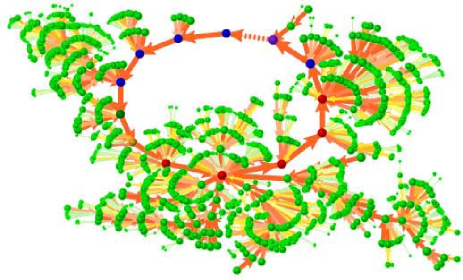
Figure 3: The probability flux. For a node, only the largest flux from it is shown. The nodes on the biological pathway are denoted with different colors: purple, the stationary G1 state; blue, the other G1 states; olive-green, S state; dandelion, G2 state; and red, M states. All other states are noted in normal green. The simulations were done with $\alpha=5$ and $\beta=6$.

We next study the statistical properties of the biological pathway of the cell-cycle network. We search the probability for the system to be in any of the biological states along the biological pathway, as a function of $\beta$. One observes a similar transition-like behavior as shown in Fig. 2. The jump of the probability of the states along the biological pathway in the low temperature phase is due to the fact that in this phase the probability flux among different states in the system is predominantly the flow along the biological pathway. To visualize this, we show in Fig. 3 an example of the probability flux among all 2048 states. Each node in Fig. 3 represents one of the 2048 states. The size of a node reflects the stationary distribution probability of the state. If the stationary probability of a state is larger than a given threshold value, the size of the node is in proportion to the logarithm of the probability. Otherwise, the node is plotted with the same smallest size. The arrows reflect the net probability flux (only the largest flux from any node is shown). The probability flux is divided into seven grades, which are expressed by seven colors: light-green, canary, goldenrod, dandelion, apricot, peach and orange. The warmer the color is, and the wider the arrow is, the larger the probability flux. The width of an arrow is in proportion to the logarithm of the probability flux it carries. The arrow representing the probability flux from the stationary G1 state to the excited G1 state (the START of the cell-cycle) is shown in dashed lines. One observes that once the system is “excited” to the START of the cell cycle process (here by noise ($\alpha$) and in reality mainly by signals like “cell size”) the system will essentially go through the biological pathway and come back to the G1 state. Another feature of Fig. 3 is that the probability flux from any states other than those on the biological pathway is convergent onto the biological pathway. Notice that this diagram also characterizes the properties of fixed points that are ignored by Li (Ref. [3]). Those fixed points also converge onto biological pathway. For $\beta<\beta_{c}$, this feature of a convergent high flux bio-pathway disappears.

In the previous discussions, we see that there is a “phase transition” as a function of the “temperature” in the stochastic cell-cycle model. The next step is to try to understand this transition-like behavior. For this purpose, we define a “potential” function and study the change of the “potential landscape” as a function of $\beta$. Specifically, we define

$$S_{n}=-\log\pi_{n}=\beta E_{n},$$ (5)

where $E_{n}$ is the pseudo energy defined in Eq. [3]. Fig. 4 shows four examples of $\Delta S_{n}=S_{n}-S0$ distribution, where the reference potential $S0$ in each plot is set as the highest potential point in the system. Note that the 11-dimensional phase space is reduced to two dimensions and there is no distance metric among the states in the 2D phase space. The states in 2D are arranged for clarity, which reflect a kind of dynamic relationship as in Fig. 3. One observes that far from the critical point ($\beta=0.01$, Fig. 4(a)), the potential values are high (around -4), and the landscape is flat. Near but below the critical point ($\beta=0.6$, Fig. 4(b)), some local minima (blue points) become more pronounced, but the landscape still remains rather flat. We notice that these minimum points do not correspond to the biological pathway. Right after the critical point ($\beta=1.5$, Fig. 4(c)), the system quickly condenses into a landscape with deep valleys [17]. The state with the lowermost potential value corresponds to the stationary G1 state. A linear line of blue dots from up-left to down-middle corresponds to the biological pathway, which forms a deep valley. Some deep blue dots out of the biological pathway are local attractors in Ref. [3]. Notice that although their potential values are low, they attract only a few nearby initial states–all these points are more or less isolated. After the critical point, the potential landscape does not change qualitatively (see Fig. 4(d) with $\beta=6$). As $\beta$, $\alpha\rightarrow\infty$, the landscape becomes nine deep holes, each corresponding to an attractor of the determinate system.

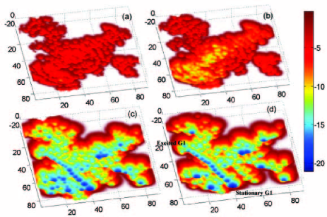
Figure 4: The “potential” landscape of the system before and after the critical point. (a) $\beta=0.01$, (b) $\beta=0.6$, (c) $\beta=1.5$, (d) $\beta=6.0$, all for $\alpha=5$. The color code gives the relative value of the potential function.

3 Conclusion

In conclusion, we introduced a stochastic model for the yeast cell cycle network. We found that there exists a transition-like behavior as the noise level is varied. With large noise, the network behaves randomly; it cannot carry out the ordered biological function. When the noise level drops below a critical value, which is of the same order as the interaction strength ($\beta_{c}\approx 1.03$), the system becomes ordered: the biological pathway of the cell cycle process becomes the most probable pathway of the system and the probability of deviating from this pathway is very small. So in addition to the dynamical and the structural stability [3], this network is also stable against stochastic fluctuations. We used a pseudo potential function to describe the dynamic landscape of the system. In this language, the biological pathway can be viewed as a valley in the landscape [18, 19, 17]. This analogy to equilibrium systems may not be generalizable, but it would be interesting to see if one can find more examples in other biological networks, which are very special dynamical systems.

4 Acknowledgments

We thanks W.Z. Ma for preparing the Fig. 4 and H. Yu for helpful discussion. This research is supported by the grants from National Natural Science Foundation of China (No. 90208022, No. 10271008, No. 10329102), the National High Technology Research and Development of China (No. 2002AA234011) and the National Key Basic Research Project of China (No. 2003CB715903)

References

- [1] K. C. Chen, A. Csikasz-Nagy, B. Gyorffy, J. Val, B. Novak, J. J. Tyson, Kinetic analysis of a molecular model of the budding yeast cell cycle, Mol Biol Cell 11 (1) (2000) 369–91.
- [2] F. R. Cross, V. Archambault, M. Miller, M. Klovstad, Testing a mathematical model of the yeast cell cycle, Mol Biol Cell 13 (1) (2002) 52–70.
- [3] F. Li, T. Long, Y. Lu, Q. Ouyang, C. Tang, The yeast cell-cycle network is robustly designed, Proc Natl Acad Sci U S A 101 (14) (2004) 4781–6.
- [4] H. C. Chen, H. C. Lee, T. Y. Lin, W. H. Li, B. S. Chen, Quantitative characterization of the transcriptional regulatory network in the yeast cell cycle, Bioinformatics 20 (12) (2004) 1914–27.
- [5] K. C. Chen, L. Calzone, A. Csikasz-Nagy, F. R. Cross, B. Novak, J. J. Tyson, Integrative analysis of cell cycle control in budding yeast, Mol Biol Cell 15 (8) (2004) 3841–62.
- [6] F. R. Cross, L. Schroeder, M. Kruse, K. C. Chen, Quantitative characterization of a mitotic cyclin threshold regulating exit from mitosis, Mol Biol Cell 16 (5) (2005) 2129–38.
- [7] B. Futcher, Transcriptional regulatory networks and the yeast cell cycle, Curr Opin Cell Biol 14 (6) (2002) 676–83.
- [8] A. W. Murray, Recycling the cell cycle: cyclins revisited, Cell 116 (2) (2004) 221–34.
- [9] N. T. Ingolia, A. W. Murray, The ups and downs of modeling the cell cycle, Curr Biol 14 (18) (2004) R771–7.
- [10] M. Tyers, Cell cycle goes global, Curr Opin Cell Biol 16 (6) (2004) 602–13.
- [11] C. V. Rao, D. M. Wolf, A. P. Arkin, Control, exploitation and tolerance of intracellular noise, Nature 420 (6912) (2002) 231–7.
- [12] M. Brun, E. R. Dougherty, I. Shmulevich, Steady-state probabilities for attractors in probabilistic boolean networks, Signal Processing 85 (10) (2005) 1993–2013.
- [13] X. Qu, M. Aldana, L. P. Kadanoff, Numerical and theoretical studies of noise effects in the kauffman model, Journal of Statistical Physics 109 (5-6) (2002) 967–986.
- [14] K. Chung, Markov chains with stationary transition probability, Springer, New York, 1967.
- [15] S. Albeverio, J. Feng, M. Qian, Role of noises in neural networks, Physical Review. E. Statistical Physics, Plasmas, Fluids, and Related Interdisciplinary Topics 52 (6) (1995) 6593–6606.
- [16] M. Qian, D. Chen, J. Feng, Metastability of exponentially perturbed markov chains, Sci. in China, Ser.A 39 (1996) 7.
- [17] Waddington, The Strategy of the Genes, Geo Allen and Unwin, London, 1957.
- [18] P. Ao, Potential in stochastic differential equations: novel construction, Journal of Physics A: Mathematical and General (3) (2004) L25–L30.
- [19] X. M. Zhu, L. Yin, L. Hood, P. Ao, Calculating biological behaviors of epigenetic states in the phage life cycle, Funct. Integr. Genomics 4 (3) (2004) 188–195.