Chaotic itinerancy, temporal segmentation and spatio-temporal combinatorial codes

Abstract

We study a deterministic dynamics with two time scales in a continuous state attractor network. To the usual (fast) relaxation dynamics towards point attractors (“patterns”) we add a slow coupling dynamics that makes the visited patterns to loose stability leading to an itinerant behavior in the form of punctuated equilibria. One finds that the transition frequency matrix between patterns shows non-trivial statistical properties in the chaotic itinerant regime. We show that mixture input patterns can be temporally segmented by the itinerant dynamics. The viability of a combinatorial spatio-temporal neural code is also demonstrated.

Several complex systems present a non-uniform rate of change, where stationary states (“patterns”) suddenly loose their stability and are substituted by new ones. Such punctuated behavior has been observed in a wide range of time scales from evolutionary, economic, social and weather dynamics, to brain behavior and laboratory devices such as laser cavities Newman1985 ; Drossel ; Kaneko2003 . Usually this “itinerancy” between states is thought as “thermal” transitions between deep valleys in a rugged landscape, possibly in the glassy dynamics regime. Such process, by definition, is stochastic so that times of transition and the choice of the next pattern are random. In this work, we consider the opposite spectrum of systems where the loss of the patterns stability is due to internal deterministic mechanisms Kaneko ; Tsuda ; Nara ; Okuda . Of course, natural systems certainly falls between these two descriptions.

The specific model studied here is a multistable system where the relevant transitions occur when a stationary state (a point attractor) looses stability so that the system falls into a new point attractor, and so on, forming an itinerant trajectory (see Fig. 1). The more general case of itinerancy between several kinds of attractors (limit cycles, torus and low dimensional chaotic attractors) has also been studied (see, for example, the special volume Kaneko2003 ).

Our model consists of a continuous state attractor network Marcus storing $P$ patterns with an added slow anti-Hebbian dynamics vanHemmen1997 ; Anderson1985 ; Hoshino (which may represent some coupling self-regulation by negative feedback). The model has a discrete time parallel dynamics with a full connected network, that is, it is a mean field coupled maps model:

$$S_{i}(t+1)=\mbox{tanh}[\gamma(h_{i}(t)+I_{i}(t))]\>,$$ (1)

where $S_{i}$, the state of neuron $i=1,\ldots,N$, is a real variable in the interval $[-1,1]$, $h_{i}$ is the local field $h_{i}(t)=\sum_{j=1}^{N}J_{ij}S_{j}(t)$, and $I_{i}(t)$ is an (eventual) external input. The parameter $\gamma$ is the transfer function gain (in this paper, $\gamma=10$). Notice that we have called the units “neurons” only by convention, since they could be better interpreted as neural populations or basic units in a network (like glomeruli in the olfactory system, species in ecological systems, population of agents in social systems etc). With this interpretations, the mean field character present in the model is more plausible.

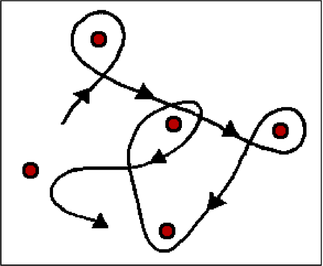
Figure 1: Schematic phase space showing an itinerant walk between point attractors.

Eq. (1) defines the dynamics for the fast variables $S_{i}(t)$ given the coupling matrix $J_{ij}$. In our model, this matrix is slowly time dependent:

$$J_{ij}(t)=J_{ij}^{H}+J_{ij}^{A}(t)\>,$$ (2)

where there is a constant Hebbian (“correlational”) component $J_{ij}^{H}$ that stores $P$ patterns, defining a basic attractor landscape, and a time dependent anti-Hebbian part $J_{ij}^{A}(t)$ that modulates this landscape and produces the escape events.

The Hebbian component has the usual form:

$$J_{ij}^{H}=\frac{1}{N}\sum_{\mu}^{P}\xi_{i}^{\mu}\xi_{j}^{\mu}\>,$$ (3)

where $\mathbf{\xi}^{\mu}=\{\xi_{i}^{\mu}\},i=1,\ldots,N;\mu=1,\ldots,P$ are random patterns to be stored. For convenience, we use binary random variables $\xi_{i}^{\mu}=\pm 1$. As usual, we set $J_{ii}=0$.

The present state $\mathbf{S}(t)$ of the system modulates the “energy” landscape (defined by slow variables $J_{ij}(t)$), so that if the system is visiting a local minimum, that minimum slowly looses its stability until turning out a saddle or a maximum and an escape event occur. The change in the attractor landscape, however, is transient, having only an exponentially decreasing memory of the past visited states. So, the anti-Hebbian component has the form

$$J_{ij}^{A}(t+1)=(1-\frac{1}{\tau})J_{ij}^{A}(t)-\frac{\epsilon}{N}S_{i}(t)S_{j}(t)\>.$$ (4)

The initial condition is $J_{ij}^{A}(0)=0$. The first term (the “coupling memory decay”) guarantees that any change produced by visiting some state vanishes with characteristic time $\tau$ after the escape from that state. The second term is the anti-Hebbian contribution, parametrized by a step size $\epsilon$ and scaled by $1/N$ to preserve compatibility with Eq. (3). So, the transition rate between patterns (or even the possibility of such transitions) depends on the two parameters $\tau$ and $\epsilon$.

The matrix $J_{ij}^{H}$ defines a permanent landscape of attractor basins that is reversibly modulated but not destroyed by the anti-Hebbian term. We notice that a similar dynamics has been studied by Kawamoto and Anderson for the particular case $P=2$ intending to model visual pattern reversion in the Necker cube Anderson1985 . Here we extend that study to general number of patterns $P$. Also Hoshino et al. Hoshino used a similar anti-Hebbian dynamics with an asymmetric coupling matrix to study transitions between fixed points and cycles. Here we are interested in the chaotic itinerancy phase that already appears with the simpler Hebbian matrix.

Our results are presented in terms of low dimensional order parameters (“overlaps”) that measure the correlation (cosine) between the state vector of the network and the stored patterns, $m_{\mu}(t)\equiv\sum_{j=1}^{N}S_{j}(t)\xi_{j}^{\mu}/(|\mathbf{S(t)}||\mathbf{\xi^{\mu}}|)$, where $|\mathbf{\xi^{\mu}}|=\sqrt{N}$ and $|\mathbf{S(t)}|$ are the vector Euclidian norms. In Fig. 2 we show an example of time series of the overlaps for $P=10$ patterns. We define an (arbitrary but not crucial) threshold $\lambda=0.8$ so that we consider that a pattern (or its anti-pattern) is being visited if $|m^{\mu}|>\lambda$. The $S(t)$ trajectory is indeed chaotic, as can be verified by observing the distance $d(t)=\sum_{i}^{N}(S_{i}(t)-S_{i}^{\prime}(t))^{2}$ between two orbits $\mathbf{S}(t)$ and $\mathbf{S}^{\prime}(t)$ with very small differences in initial conditions (Fig. 3).

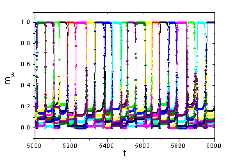
Figure 2: Time series of overlaps moduli $|m^{\mu}|$ for $P=10$, with $\epsilon=0.009$, $\tau=600$ and $N=100$.

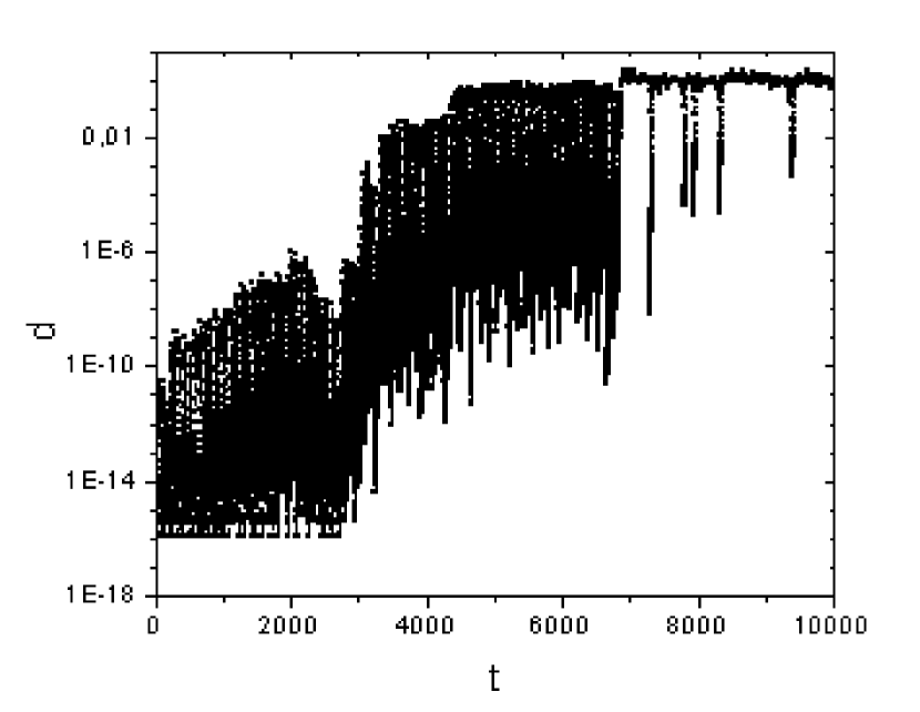
Figure 3: Distance between trajectories $d(t)$ as a function of time. The two systems have identical initial coupling matrixes and differ only in the first neuron, $|S_{1}(0)-S_{1}^{\prime}(0)|=10^{-15}$.

From the time series one gets the symbolic time series where only appears the pattern (if any) being visited (Fig. 4). Although we report here only simulations with $N=100$ and $\alpha=P/N=0.1$, we have checked that the itinerancy occurs until a effective critical storage $\alpha_{c}\propto 0.2$. This value is higher than the standard critical capacity $\alpha_{c}=0.14$ due to the effect of the anti-Hebbian term which is similar to unlearning algorithms vanHemmen1997 .

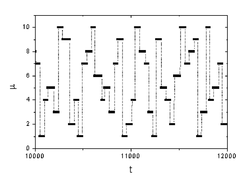
Figure 4: Label of the visited pattern as a function of time. The system itinerates chaotically but with almost equal frequency between the stored patterns ($P=10$ and $N=100$).

From extensive symbolic time series one obtains statistics about transitions and residence times (Fig 5). A not so obvious result is that, in a large parameter region, all patterns are visited with almost equal frequency (Fig. 5 inset). This finding is similar to that found in Nara model Nara .

We define $T_{\mu\nu}$ as the relative frequency matrix of transitions from pattern $\nu$ to pattern $\mu$. In simple stochastic trap models Bouchaud ; Martinez2004 the $T_{\mu\nu}$ elements are similar (there is no preferential transitions between attractors). In our deterministic model, in contrast, the transition matrix is very inhomogeneous, as can be seem by a rank plot of $T_{\mu\nu}$ values (Fig. 5).

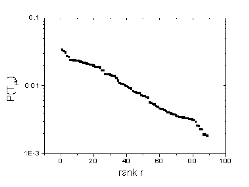
Figure 5: Rank plot of the values of the transition frequencies $T_{\mu\nu}$. Inset: Average residence times near each pattern.

Up to now we have reported the presence of chaotic itinerancy between the stored patterns without external input ($I_{i}=0$). This corresponds to a spontaneous itinerant network activity, as devised by Freeman Freeman . This author postulates that, under the presence of some input, the chaotic itinerancy should collapse to an attractor of lower dimension representing that input. Our model is a computational implementation of Freeman’s ideas. A new feature is that this lower dimensional attractor also has a chaotic itinerant nature (with less components).

Think about a mouse receiving a complex mixture of odours (each odour being represented by an initial pattern in its olfactory glomeruli layer). Galan et al. have recently observed experimentally that glomerulli show Hebbian (correlational) plasticity, and that a Hopfield network is a viable model of the glomerular layer Galan . Following Adachi et al.AAC , we propose that chaotic itinerancy between input components may be a mechanism to analyse such complex input by using temporal segmentation. In a loose sense, we have a chaotic itinerancy projected into the subspace spanned by the patterns that compose the mixture input vector AAC ; Matykiewicz .

In Fig. 6a we show the network response to inputs made of a mixture of $Q$ patterns $I_{i}=(H/\sqrt{Q})\sum_{\nu=1}^{Q}\xi_{i}^{\nu}$, where the input intensity is $H$. In Fig. 6b we have a bifurcation plot as a function of $H$ showing that there is a robust interval where the system itinerates only between the $Q$ vectors that form the total input. This result is generic in parameter space and is valid from $Q=1$ up to $Q=0.6P$. This means that the system makes a temporal segmentation even if the input is composed by an extensive number of patterns. For increasing odor intensity $H$ the nature of itinerancy changes following a series of plateaus. We conjecture that this could be the theoretical correlate of a well known phenomenon where smells change abruptly of subjective character as a function of odour concentration smell .

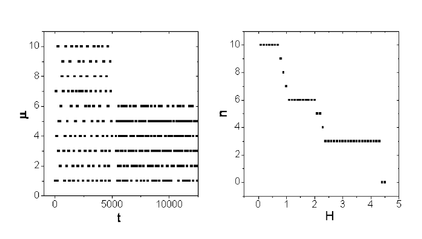
Figure 6: a) Network response to an input composed by $Q=6$ patterns ($\mu=1$ to $\mu=6$) with $H=1.2$. The input starts at $t=5000$. b) Total number of patterns visited as a function of the input intensity $H$. Notice that for $n\leq 6$, all patterns are input components.

Although temporal segmentation is an intersting feature of the model, the more recent view is that odours are represented as sequences of patterns of glomerular activation, that is, a spatio temporal combinatorial code Laurent ; Cleland . The model allows such interpretation, if we think the patterns $\xi^{\mu}$ as being not odour representations but as forming a basis to combinatorially represent odours. In this scenario, we have upt to $C=P!/(Q!(P-N)!)$ possible representations with $Q$ components. For example, with a typical vertebrate glomerular layer with $N=1000$ glomeruli and assuming $P=50$ and $Q=3$ (that is, odours will be represented as sequences of three patterns), we have $C=\approx 20,000$ odours, which is already above the conjectured number of odours recognized by mammals.

Another possible application for chaotic itinerancy phenomena is as a theoretical framework for understanding multistability in visual phenomena Multistability . Here, an ambiguous figure would correspond to a mixture input where the $Q$ components are the $Q$ possible interpretations of the figure (see Fig. 7). Visual multistability phenomena will be studied computationally and experimentally in another work. A preliminary finding is that, both in the model and in experiments, the transition frequency between patterns grows with $Q$, showing that competition between the $Q$ patterns (and not only fatigue factors) modulates the rate of transition between patterns.

Figure 7: Example of visual multistability Multifigure where transitions between several patterns can be observed.

Our model differs from previous itinerant systems in regard to:

• In contrast to Kaneko coupled lattices Kaneko , the number $P$ of quasi-attractors (patterns) can be set in advance and a study in function of $\alpha=P/N$ can be done;

• Differently from Nara model Nara , we do not need to dilute the network to obtain itinerancy. This preserves a large capacity $\alpha_{c}$ without requiring sophisticated (pseudo-inverse) learning matrixes. This large capacity (and larger stability of each individual pattern) enables us to show that pattern separation (by temporal segmentation) can be done for inputs with a high level of mixture (up to $0.6\alpha$ or higher). This should be contrasted to very recent attempts of using chaotic itinerancy for pattern separation where mixture inputs have only two or three components Matykiewicz ;

• In contrast to Aihara Aihara and Kaneko Kaneko models, we do not need to use individual chaotic elements to obtain global chaotic itinerancy. We think that it is important to stress this point: chaotic itinerancy and local chaos are independent concepts;

• Of course, the advantages have a price: our system is composed of a $O(N^{2})$ number of equations in contrast to $O(N)$ equations of previous itinerant systems.

We notice that the same anti-Hebbian process can be implemented in other rugged landscapes systems like, for example, a Sherrington-Kirkpatric (SK) model with zero temperature parallel dynamics. We expect a similar or more complex itinerant evolution due to the exponential number of minima in these systems. In such spin glass-like system, however, since we do not know a priori where the minima lie, we may study energy and autocorrelation functions instead of the overlap $m_{\mu}(t)$ available in neural networks systems. In these systems, our anti-Hebbian slow process could be though as an energy paving search method with some similarity to other methods proposed in the literature Hansmann .

A final observation is that we studied only the itinerant “equilibrium regime”, meaning that in the parameter region examined the transition frequency matrix appear to have a time independent form. However, for small step sizes $\epsilon$, one should expect a scenario where the overall trajectory is transient, stopping at the most stable attractors. So, transient itinerant dynamics could be relevant as an alternative proposal for fast (non thermal) dynamical mechanism to produce convergence to a “native” state in the protein folding problem. It is also conceivable an out of equilibrium “glassy” scenario, probably in the large $\alpha$ regime, where the residence times may strongly depend on the relative stability of the local minima and the mean residence time diverges like in trap models Bouchaud ; Martinez2004 .

Out-of-equilibrium chaotic itinerancy is a topic for future work. These transient and glassy regimes are of interest because the complex time evolutions of the biological or socio-economical systems cited in the introduction are primary examples of such out-of-equilibrium (“historical”) dynamics. As at least one concrete suggestion for these problems, our study illustrates the idea that the competitio (“dialectics”) between short term stabilizing and long term corrosive internal factors is a sufficient conditions to produce a punctuated, revolutionary history where, even following a deterministic dynamics, future is not predictable.

Acknowledgments: Research supported by FAPESP, CNPq and CAPES. We acknowledge discussions with I. Tsuda, A. Roque da Silva, P. Zambianchi, bibliographic aid from M. Adachi and K. Aihara and C. F. Schmidt for allowing the use of figure 7.

References

- (1) C. M. Newman, J. E. Cohen, and C. Kipnis, Nature 315, 400 (1985).
- (2) B. Drossel, Adv. Phys 50(2), 209 (2001).
- (3) K. Kaneko and I. Tsuda, Chaos 13(3), 926 (2003).
- (4) K. Kaneko, Phys. Rev. Lett. 78, 2736 (1997).
- (5) I. Tsuda, Behav. Brain Sci. 24, 793 (2001).
- (6) S. Nara and P. Davis Prog. Theoret. Phys. 88, 845 (1992).
- (7) H. Okuda and I. Tsuda, Int. J. Bifurcation Chaos 4, 1011 (1994).
- (8) C. M. Marcus, F. R. Waugh, and R. M. Westervelt, Phys. Rev. A 41, 3355 (1990).
- (9) J. L. van Hemmen, Network: Comput. Neural Syst. 8, V1-V17 (1997).
- (10) A. H. Kawamoto and J. A. Anderson, Acta Psychol. 59, 35 (1985).
- (11) O. Hoshino, Y. Kashimori, and T. Kambara. PNAS textbf93, 3303 (1996).
- (12) R. A. Denny, D. R. Reichman, and J.P. Bouchaud Phys. Rev. Lett. 90, 025503 (2003).
- (13) Martinez A. S., Kinouchi O., and Risau-Gusman S., Phys. Rev. E. 69, 017101 (2004).
- (14) C. H. Skarda and W. Freeman, Behav. Brain Sci. 1, 161 (1987).
- (15) R. F. Galan, M. Weidert, R. Menzel, A. V. Herz, and C. G. Galizia, Neural Comput. 18, 10 (2006).
- (16) M. Adachi, K. Aihara, and A. Cichocki, in International Symposium on Nonlinear Theory and its Application (NOLTA), Katsurahama-so, Kochi, Japan 93 (1996).
- (17) P. Matykiewicz, ICAISC 2004 Lecture Notes in Artificial Intelligence 3070, 235 (2004).
- (18) Laurent, G. Nat. Rev. Neurosci. 11, 884 (2002).
- (19) T. A. Cleland and C. Linster Chem. Senses 30, 801 (2005).
- (20) R. Gross-Isserof and D. Lancet, Chem. Senses 13,191 (1988).
- (21) Wright GA, Thomson MGA, Smith BH Proc. Royal Society B - Biol. Sci. 272, 2417 (2005).
- (22) D. A. Leopold, M. Wilke, A. Maier, and N. K. Logothetis, Nat. Neurosci. 5, 605 (2002).
- (23) The figure has been downloaded from http://www.rci.rutgers.edu/
- (24) M. Adachi M. and K. Aihara, Neural Networks 10, 83 (1997).
- (25) U. H. E. Hansmann and L. T. Wille, Phys. Rev. Lett. (88), 068105 (2002).