Physics-based analysis of Affymetrix microarray data

Abstract

We analyze publicly available data on Affymetrix microarrays spike-in experiments on the human HGU133 chipset in which sequences are added in solution at known concentrations. The spike-in set contains sequences of bacterial, human and artificial origin. Our analysis is based on a recently introduced molecular-based model [E. Carlon and T. Heim, Physica A 362, 433 (2006)] which takes into account both probe-target hybridization and target-target partial hybridization in solution. The hybridization free energies are obtained from the nearest-neighbor model with experimentally determined parameters. The molecular-based model suggests a rescaling that should result in a “collapse” of the data at different concentrations into a single universal curve. We indeed find such a collapse, with the same parameters as obtained before for the older HGU95 chip set. The quality of the collapse varies according to the probe set considered. Artificial sequences, chosen by Affymetrix to be as different as possible from any other human genome sequence, generally show a much better collapse and thus a better agreement with the model than all other sequences. This suggests that the observed deviations from the predicted collapse are related to the choice of probes or have a biological origin, rather than being a problem with the proposed model.

I Introduction

DNA microarrays Schena et al. (1995) allow to measure the gene expression level of thousands of genes simultaneously. This is a major step forward compared to traditional methods in molecular biology (as Northern blots) which are applicable only to a limited set of genes at a time. The determination of gene expression levels is not the only application of DNA microarrays, which have been used also for the analysis of genetic variance between individuals (single nucleotide polymorphisms), as efficient tools for DNA sequencing, for the study of chromosomal defects and for the determination of alternative splicing events.

Despite the increasing popularity that microarrays have known in the recent years there are still some problems with the technology. There has been, for instance, only a moderate effort in comparing different microarrays platforms on the same biological system Marshall (2004). When this comparison was made, as in a recent study on expression analysis of stressed-out pancreas cells, it was found that different commercial platforms produced wildly incompatible data Tan et al. (2003). These problems call for a better fundamental understanding of the functioning of the microarrays. Such understanding will help researchers to design better algorithms for microarray data analysis based on the physical-chemistry of the underlying hybridization process.

In the past years several experiments were addressing the analysis of equilibrium and dynamical properties of DNA hybridization to probes anchored on solid surfaces with different techniques as, for instance, surface plasmon resonance Peterson et al. (2002) and by quartz microbalance Okahata et al. (1998). At the same time several papers Vainrub and Pettitt (2002); Held et al. (2003); Naef and Magnasco (2003); Hagan and Chakraborty (2004); Halperin et al. (2004); Binder and Preibisch (2005); Carlon and Heim (2006) have been dedicated to theoretical aspects of hybridization, mostly discussing the Langmuir model and variances thereof.

In a previous paper Carlon and Heim (2006) we have analyzed a series of publicly available data of experiments performed on Affymetrix microarrays, using a simple model of the hybridization process. In these experiments a set of selected genes are “spiked-in” at fixed concentrations into a solution containing other types of RNAs. This set of data has been widely used as testground for algorithms designed to extract gene expression levels from the raw data. Affymetrix is one of the major commercial producers of microarrays. In Affymetrix arrays the surface-bound probes are prepared in situ by photolitographic techniques. Although the technique is limited to rather short oligos (25 nucleotides long) one of the advantages is that a high density of probe sequences per array can be obtained. In the latest generation 1,400,000 different probes have been placed in a single array. The large number of probes compensate for their limited length. Indeed Affymetrix uses multiple probes per gene, which define a probe set. Another special feature of Affymetrix chips is that it uses as control a mismatch (MM) probe sequence, which differs from a perfect-matching (PM) sequence only at the base at position 13: a nucleotide A is interchanged with T and a nucleotide C is interchanged with G.

In our previous work Carlon and Heim (2006) we focused on the spike-in data set of the HGU95 human chipset. More recently this has been substituted by the HGU133 chipset. Probe sets have been completely redesigned in the HGU133 chipset; moreover there are only 11 probes per probe set compared to the 16 probes of the HGU95 array. In this paper we focus on the analysis of publicly available spike-in data on the HGU133 chip, building on our previous work Carlon and Heim (2006) on HGU95. This will allow us to test the robustness of the model introduced in Ref. Carlon and Heim (2006) to a new set of data. There is another interesting feature of the spike-in data of the HGU133 chipset: differently from the HGU95 data where spikes correspond to human genes, the spikes in the HGU133 have been selected between human, bacterial and “artificial” sequences. The latter were selected by Affymetrix to avoid cross-hybridization with any known human coding sequence.

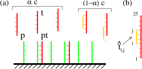
Figure 1: (a) The simple model of hybridization in Affymetrix microarrays used throughout this paper is defined by two basic reactions: 1) Hybridization between target molecules (t) to surface anchored probes (p) leading to a duplex pt and 2) The hybridization between target molecules in solution leading to the partial duplexes $t{\hat{t}}_{i,j}$. In the model, the effect of the hybridization in solution amounts to a reduction of the original target concentration $c$ to a value $\alpha c$. (b) Partial hybridization of a fragment in solution complementary to the target RNA sequence from base $i$ to base $j$ ($1\leq i<j\leq 25$).

II A simple model for hybridization in Affymetrix arrays

In this section we briefly recall the model introduced in Ref. Carlon and Heim (2006). Two basic processes are considered: 1) Target-probe hybridization and 2) Target-target hybridization in solution. According to the model the fluorescence signal measured from a given probe is:

$$I=I_{0}+\frac{A\alpha ce^{\beta\Delta G}}{1+\alpha ce^{\beta\Delta G}}$$ (1)

where $I_{0}$ indicates a background level due to non-specific hybridization, $A$ sets the scale of intensities, $c$ is the target concentration (a measure of the gene expression level), $\Delta G$ the target/probe hybridization free energy, $\beta=1/RT$ the inverse temperature, $R$ the universal gas constant. Here, $\alpha$ models the reduction in the concentration of available targets due to the target-target hybridization in solution: only a fraction $\alpha c$ is available for the hybridization with probes as the remaining $(1-\alpha)c$ form stable duplexes with other partners in solution (see Fig. 1(a)).

In the model introduced in Ref. Carlon and Heim (2006), we approximate the target-target hybridization with the expression

$$\alpha\approx\frac{1}{1+\tilde{c}\exp{\left(\beta^{\prime}\Delta G_{R}^{(37)}\right)}}$$ (2)

with $\beta^{\prime}$ and $\tilde{c}$ fitted parameters and $\Delta G_{R}^{(37)}\equiv\Delta G_{R}(1,25)$ the (sequence dependent) RNA/RNA free energy for duplex formation in solution at 37 degrees calculated over the whole 25-mer length; in close approximation, the binding free energies at 37 and 45 degrees (the actual experimental temperature) are almost identical, apart from a small scaling factor, which is adsorbed into the rescaled temperature $\beta^{\prime}$. In the next section, we will discuss the steps leading to Eq. (2) in more detail.

The model defined in Eqs. (1) and (2) contains the four fitting parameters $A$, $\beta$, $\beta^{\prime}$ and $\tilde{c}$ which were fitted against the spike-in data of the Affymetrix array HGU95a in Ref. Carlon and Heim (2006). The parameters $\beta^{\prime}$, $\tilde{c}$ and $A$ will be discussed in Sec. III and Sec. IV. The parameter $\beta$ is the inverse temperature. Instead of fixing it to the experimental value we have kept it as a fitting parameter as explained in Ref. Carlon and Heim (2006). The hybridization free energies $\Delta G$ and $\Delta G_{R}$ are calculated from tabulated experimental data for DNA/RNA Sugimoto et al. (1995, 2000) and RNA/RNA Xia et al. (1998) duplex formation in solution.

We note that we fit mismatches and perfect matches with the same model. The difference between the two is that there is a different hybridization free energy $\Delta G$: one expects a lower signal for mismatches compared to perfect matches, due to weaker binding. This is not always the case; as remarked in several studies for a substantial fraction of probes (30%, as reported in Ref. Naef and Magnasco (2003)) one observes “bright mismatches” for which the mismatch intensity $I_{\rm MM}$ exceeds the intensity $I_{\rm PM}$ of the perfect match. However, it has been observed Binder and Preibisch (2005) that bright MM come predominantly from probes with low intensity, which suggests that bright mismatches are associated with weak specific hybridization when the signal $I$ is dominated by $I_{0}$ in Eq. (1).

In recent work Heim et al. (2006) we also compared the current model with the approach based on position-dependent effective affinities as for instance described in Refs. Naef and Magnasco (2003); Binder and Preibisch (2005). The conclusion is that the two approaches are fully consistent with each other, provided that various effects are incorporated such as partial unzipping of the probe-target complex, less than 100% efficiency in the probe growth during lithography, and entropic repulsion between the target and the substrate. These additional effects are the main factors causing position-dependence (and thus allowing for a comparison with position-dependent effective affinities); for a quantitative prediction of the intensities, their combined effect can be well approximated by a slight decrease of $\beta$ in Eq. (1) and they are therefore not included in the current study.

III On the hybridization in solution

We now discuss the approximations leading to the form of $\alpha$. We denote the concentration of free 25-mer targets in solution as $[t]$, the concentration of free target strands that are complementary from nucleotide $i$ up and including nucleotide $j$ as $[\hat{t}_{i,j}]$, and the concentration of duplexes between these two as $[t\,\hat{t}_{i,j}]$. Chemical equilibrium (see Fig. 1(b)) yields for the equilibrium constant:

$$K_{i,j}=\frac{[t][\hat{t}_{i,j}]}{[t\hat{t}_{i,j}]}=e^{-\beta\Delta G_{R}(i,j)},$$ (3)

where $\Delta G_{R}(i,j)$ is the RNA/RNA hybridization free energy for target molecules in solution, which are complementary from nucleotide $i$ up and including $j$, and $\beta=1.59$ mol/kcal (corresponding to the experimental temperature of 45 degrees). For a given gene, the measure of the gene expression level which one wants to determine is the total target concentration $c$ given by

$$c=[t]+\sum_{i,j}[t\hat{t}_{i,j}].$$ (4)

Solving Eqs.(4) and (3) we find for the fraction of single stranded target in solution:

$$\alpha_{f}=\frac{[t]}{c}=\frac{1}{1+\sum_{i,j}[\hat{t}_{i,j}]\exp(\beta\Delta G_{R}(i,j))}.$$ (5)

Note that the summation in the denominator of Eq. (5) was replaced in the approximate expression Eq. (2) by the single term $\tilde{c}\exp(\beta^{\prime}\Delta G_{R}^{(37)})$, with fitting parameters $\tilde{c}$ and $\beta^{\prime}$.

Eq. (5) requires as input estimates of the concentration $[\hat{t}_{i,j}]$ of complementary sequences with length $l=j-i+1$, present in solution. Assuming that all four nucleotides are roughly equally abundant, and that there are no correlations along the sequence, the abundance of short sequences with length $l$ will decrease as $[\hat{t}_{i,j}]\sim 4^{-l}$. This scaling breaks down beyond some length $L$; assuming for the human transscriptome a total length of $10^{7}$ nucleotides, a random sequence longer than 12 is more likely not present at all, since $4^{12}\gtrsim 10^{7}$. We therefore take as our approximation

$$[\hat{t}_{i,j}]=\left\{\begin{array}[]{cc}c_{0}\cdot 4^{-(j-i)}&{\rm for\ j-i<12,}\\ 0&{\rm otherwise.}\end{array}\right.$$ (6)

Here, $c_{0}$ is a measure of the RNA concentration. Using this approximation for the concentration of complementary strands, we can now compare Eqs. (2) and (5). Fig. 2 shows the more elaborate model Eq.(5) as a function of the approximate form Eq. (2), with the values for the fitting parameters $\beta^{\prime}$ and $\tilde{c}$ taken from Ref. Carlon and Heim (2006). There is a reasonable agreement between the two.

Figure 2: Comparison of the summation in Eq. (5), equal to $\alpha_{f}^{-1}-1$, and its approximation in Eq. 2), equal to $\alpha^{-1}-1$, for the first 1,000 spike-in sequences of HGU133. Note that a change in $c_{0}$ corresponds to a vertical shift over $\log(c_{0})$; in this figure, we used $c_{0}=1$. The straight line is a fit, given by $y=x+b$ with $b=-14.1$.

Since Eq. (5) has a better microscopic foundation than Eq. (2), it should in principle allow for a better estimate of the hybridization in solution. There are however severe limitations to the use of Eq. (5). In the hybridization in solution, there is a competition between the contributions of short sequences, which are abundant but have a low affinity, versus long sequences, for which the concentration is low but the affinity high. The concentration drops on average approximately by a factor of 4 per added length (see Eq. (6)), but the affinity grows by approximately $\langle\Delta G\rangle\approx$ 2 or 3 kcal/mol, the average value of RNA/RNA interaction parameters Bloomfield et al. (2000). Since $\exp(\beta\langle\Delta G\rangle)>4$, the longer sequences dominate the hybridization in solution. However, as discussed above, beyond length $L\approx 12$, there simply are no complementary strands. The accuracy of the more elaborate model Eq. (5) thus hinges crucially on knowing the longest complementary strand which is transcribed, as well as its affinity and its concentration. Since the approximate model Eq. (refalpha) is not expected to perform worse than the more elaborate model Eq. (5), we keep using the former.

The data points in Fig. 2 can be fitted by a straight line with slope 1: the value of $\beta^{\prime}=0.67$ mol/kcal in Ref.Carlon and Heim (2006), corresponding to 725 K, apparently is the appropriate value to describe the experiments at a temperature of 45 degrees. The offset in the straight-line fit is equal to $\log(\tilde{c})-\log(c_{0})$. Since the straight-line fit has an offset of -14.1, and since we used the fitted value of $\tilde{c}=2\cdot 10^{-2}pM$ in Ref. Carlon and Heim (2006), an estimate of the RNA concentration is $c_{0}=\exp(14.1)\cdot\tilde{c}=30$ nM. Even if we do not use the more elaborate model Eq. (5), it provides us with a microscopic basis for the values of the parameters $\beta^{\prime}$ and $\tilde{c}$ in the approximate model Eq. (2).

Figure 3: Plot on intensity vs. concentration for three spike-in genes of the HGU133 chipset. $I_{\rm max}$ indicates the saturation value obtained from a three parameters ($I_{0}$, $A$ and $K$) non-linear fit based on Eq. (8).

IV On the signal saturation level

If the target concentration $c$ and the binding energy $\Delta G$ are sufficiently high, the Langmuir isotherm saturates to a maximal value. From Eq. (1) we find for $c\exp(\beta\Delta G)\gg 1$

$$I_{\rm max}=I_{0}+A\approx A,$$ (7)

where we have used the fact that typically the background level, $I_{0}$, is much lower than the value of $A$. The saturation intensity arises if targets are bound to almost all probes. Since the number of probes does not vary between the sequences being measured, this saturation intensity is also expected to be sequence-independent, and more specifically, should not distinguish between perfect matches and mismatches. A recent analysis of the Latin square set Held et al. (2003); bur reported widely different values for the saturation intensity. It is worth clarifying further this issue here.

The obvious procedure to determine the saturation intensity, is to look at the intensity of a probe as a function of concentration. Assuming an effective affinity $K_{s}$ for probe sequence $s$, the intensity $I_{s}(c)$ as a function of concentration $c$ is given by

$$I_{s}(c)=I_{0,s}+\frac{A_{s}cK_{s}}{1+cK_{s}},$$ (8)

in which $I_{0,s}$ is the (sequence-dependent) background intensity due to non-specific binding. A plot of $I_{s}$ vs. $c$ for two probes of the HGU133 spike-in set is shown in Fig. 3. Taking $I_{0}$, $A$ and $K$ in eq. (8) as fitting parameters, and extrapolating to high concentration then yields the saturation intensity.

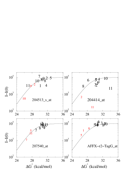
Figure 4: Plot of $I-I_{0}$ as a function of $\Delta G-RT\log\alpha$ for 4 sequences spiked-in at a concentration of $c=512$ pM. The numbers indicate the probe set numbers. Smaller characters are used for the MM signals. Solid lines represent the Langmuir model as given by Eq. (2). The data are consistent, except few outliers, with the Langmuir model with roughly constant saturation level $A\approx 10^{4}$.

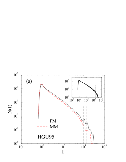
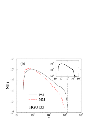
Figure 5: Histograms of the PM and MM intensities for the Latin square experiments in log-log scale for the chips HGU95a (a) and HGU133 (b). The plots contain 19 histograms referring to different experiments (a) and 12 experiments (b). The dashed lines are positioned at $I=10000$ and $I=15000$ (intensities are given in Affymetrix scale). Insets: histograms of the total intensity of PM and MM together.

Two research groups Held et al. (2003); bur followed this procedure, and both found saturation intensities that vary wildly between different sequences. A first effect that can cause deviations from the Langmuir fit Eq. (8) is that the lithographic process, through which the probes are synthesized in situ in Affymetrix chips, is not 100% efficient. As estimated by Burden bur , only about 10% of the probes reach the full length of 25 nucleotides. At low intensities far from saturation, the incomplete probes can be safely ignored since their affinity is much lower than that of the fully grown probes. However, under conditions where the fully grown probes are saturated, clearly there will be contributions to the fluorescent intensity from the almost complete probes, and an even further increase in concentration will bring into play shorter and shorter incomplete probes. Consequently, the Langmuir fit Eq. (8) breaks down near saturation; extrapolation to high concentration is an unreliable procedure.

A second cause of worry is that comparing fluorescent intensities from different chips is also potentially unreliable, since the microarrays might have undergone slightly different processing during the washing and staining. Since Affymetrix microarrays cannot be reused, the spike-in measurements used in Refs. Held et al. (2003); bur required a new chip for each concentration.

To avoid these two potential sources of error, we therefore consider the intensities for a given probe set at a specific concentration, i.e. $c$ constant and $\Delta G$ and $\alpha$ variables in Eq. (1). The data belong to the same array. An example of this type of analysis is shown in Fig. 4 for a concentration of $c=512$ pM. On the horizontal axis we plot $\Delta G^{*}=\Delta G-RT\log\alpha$. The solid lines are given by the Langmuir curve Eq. (1). Note that the large majority of the probes align along the expected curve, with few exceptions as for instance probe 11 (both PM and MM) for the probe set 204414_at. Therefore, the data are consistent with a value of $A$ roughly constant in Eq. (1), which suggests indeed that the large variations in $I_{\rm max}$ obtained from the extrapolations of the data in the earlier analysis are more likely to be an artifact of the extrapolations. Note however that some variability of the saturation level can be seen in the data of Fig. 4. Typically this variability is of about $20\%$. In order to keep the model simple we will keep $A$ constant in the rest of the paper. An interesting possible explanation of the variability of $A$ has been given in Ref. bur , i.e. that this variation is due to the post-hybridization washing of the array.

Yet another different way of addressing the issue of the saturation intensities is to analyze the histogram of the intensities on the whole chip, as in Fig. 5, which shows both the intensities for the HGU95 and HGU133 spike-in data. To reveal the data at high intensities, they are plotted in a log-log scale. In the figure we note a drop in the histogram around $I\approx 10\ 000$, sharper in the HGU133 chipset, which is consistent with the estimate of the saturation intensity obtained from the fits of intensities vs $\Delta G-RT\log\alpha$, as given in Fig. 4. Note that in Fig. 5(b) the drop is 100-fold in the range $10\ 000<I<15\ 000$, which suggests that the data are consistent with a roughly constant value of the saturation. However a more close inspection of the histogram of the HGU133 for PM and MM intensities separately, reveals that the estimated saturation value for the two may be different. In the case of PM intensities alone the drop is rather sharp at around $I\approx 10\ 000$, however the MM intensities seem to saturate at lower intensities, which is not seen in the HGU95 data (Fig. 5(a)). The number of MM probes reaching an intensity close to the saturation level in the histogram of Fig. 5(b) is quite small so the fact that the the MM and PM reach a different saturation level cannot be concluded for sure.

Also the low-intensity side of the histograms in Fig. 5 contain interesting information. Both for the HGU95 and HGU133, the intensity drops steeply below a minimal intensity. For HGU95, this drop occurs around $I_{\rm min}\approx 70$, while for HGU133 the drop occurs around $I_{\rm min}\approx 30$. This increase of the dynamical intensity range by more than a factor of two is a clear demonstration of the fast rate of improvement in microarray technology.

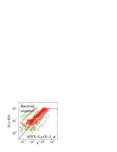
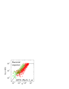
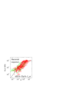
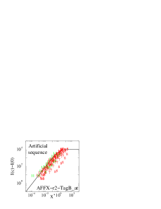
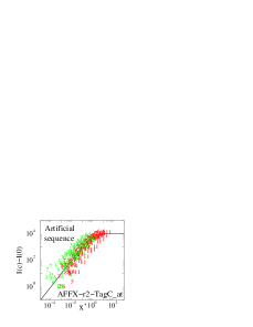
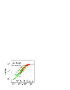
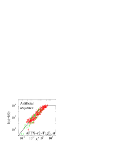
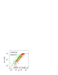
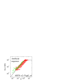
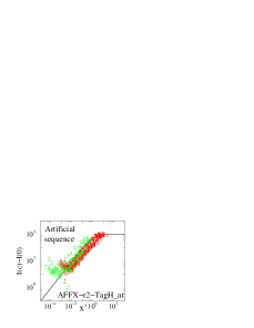
Figure 6: Collapse plots for the 4 bacterial and the 8 artificial sequences of the HGU133 spike-in set. In these plots the background subtracted intensities for a given probe set are plotted as functions of the rescaled variable $x^{\prime}$ given in Eq. (9). The data corresponds to all spike-in concentrations for a given probe sets. Solid lines correspond to the Langmuir isotherm. Compared with the human and bacterial sequences the artificial sequences are characterized by the best collapses.

V Analysis of data collapses

As a test of the validity of the model we plotted Carlon and Heim (2006) the data as a function of the rescaled variable:

$$x^{\prime}=\alpha ce^{\beta\Delta G}.$$ (9)

If the model is to be trusted the data for different values of $c$ and different probe sequences (i.e. different $\Delta G$ and $\alpha$) ought to “collapse” onto a single master curve

$$I-I_{0}=\frac{Ax^{\prime}}{1+x^{\prime}}.$$ (10)

This collapse has indeed been observed in the large majority of the spike-in genes of the HGU95a chipset Carlon and Heim (2006). Interestingly, the very few outliers observed in that case could be explained as annotation errors or unbalance of free energies used for specific nucleotides, as discussed in Ref. Carlon and Heim (2006).

We choose here the same fitting parameters used in Ref. Carlon and Heim (2006) for the HGU95 chipset, that is: $A=10\ 000$, $\beta=0.74$ mol/kcal, $\beta^{\prime}=0.67$ mol/kcal and $\tilde{c}=10^{-2}$ pM. These parameters fit equally well the HGU133 spike-in data.

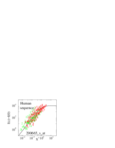
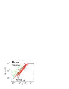
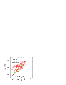
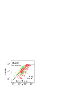
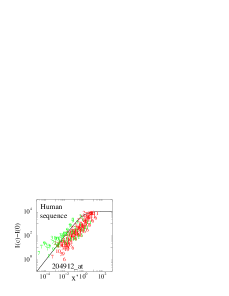
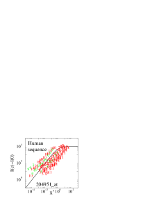
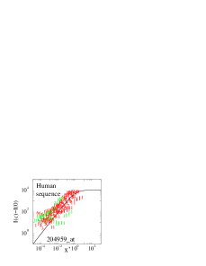
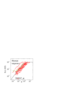
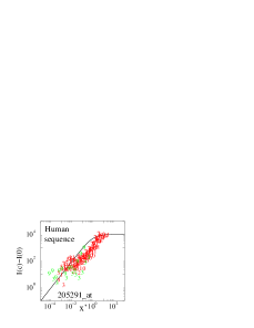
Figure 7: Collapse plots for Human sequences of the HGU133 spike-in set (part 1). The probes which are complementary to targets which the largest folding free energies are emphasized (see Table 3). They correspond to probes 204912_at10 and 204513_s_at4.

Table 1: List of values of $\langle w\rangle$ and $\sigma_{w}$ for the bacterial and the artificial sequences in the spike-in set HGU133.

Probe set	$\langle w\rangle$	$\sigma_{w}$	Probe set	$\langle w\rangle$	$\sigma_{w}$
AFFX-DapX-3_at	0.08	1.49	AFFX-PheX-3_at	0.16	1.55
AFFX-LysX-3_at	0.89	2.46	AFFX-ThrX-3_at	0.22	1.59
AFFX-r2-TagA_at	-1.05	0.97	AFFX-r2-TagE_at	-0.32	0.82
AFFX-r2-TagB_at	-0.51	0.83	AFFX-r2-TagF_at	-0.46	1.09
AFFX-r2-TagC_at	0.43	1.08	AFFX-r2-TagG_at	-0.11	0.90
AFFX-r2-TagD_at	-0.03	0.90	AFFX-r2-TagH_at	0.11	1.22

Table 2: List of values of $\langle w\rangle$ and $\sigma_{w}$ for the human sequences in the spike-in set HGU133.

Probe set	$\langle w\rangle$	$\sigma_{w}$	Probe set	$\langle w\rangle$	$\sigma_{w}$
200665_s_at	0.54	1.26	205569_at	-0.28	1.12
203471_s_at	0.39	1.43	205692_s_at	0.24	1.27
203508_at	0.45	1.83	205790_at	-0.78	0.76
204205_at	0.86	2.11	206060_s_at	0.52	1.66
204417_at	-0.24	1.18	207160_at	-0.32	1.06
204430_s_at	-0.48	1.13	207540_s_at	-0.29	0.62
204513_s_at	-0.68	1.16	207641_at	0.24	2.72
204563_at	-0.57	1.44	207655_s_at	0.76	1.06
204836_at	-0.04	1.41	207777_s_at	-0.14	1.11
204912_at	-0.31	1.35	207968_s_at	-0.85	1.66
204951_at	-0.15	1.48	209354_at	0.04	1.41
204959_at	1.33	1.62	209606_at	0.77	1.44
205267_at	0.36	1.23	209734_at	-0.20	1.51
205291_at	-0.44	1.24	209795_at	0.63	1.71
205398_s_at	-0.15	1.37	212827_at	0.61	2.53

In Figs. 6, 7 and 8 we show the collapse plots for all the 42 genes of the spike-in data set HGU133. Each plot contains about 200 points, which all tend to cluster (in some cases much better than others) along the Langmuir curve $Ax^{\prime}/(1+x^{\prime})$. All the 13 concentrations, which range from $0.125$ pM to $512$ pM in the spike-in experiment, are shown. The intensities measured at $c=0$ are taken as estimates of the background level $I_{0}$ in Eq.(10). In the collapse plots only the MM sequences for which a $\Delta G$ could be estimated are shown, as the mismatch free energies in RNA/DNA duplexes are known only for a limited set of mismatches Sugimoto et al. (2000) (we could associate a free energy to about 30% of mismatches, as discussed in Ref. Carlon and Heim (2006)).

The HGU133 spike-in set contains 4 bacterial sequences and 8 artificial sequences (Fig. 6) and 30 human sequences (Fig. 7 and 8). A perfect agreement with the Langmuir theory would imply that the data all align along the curve given by Eq. (10) and shown as a solid line in the Figs. 6, 7 and 8. In general the agreement is best for the artificial sequences. Occasionally, also some human sequences collapse well into a single curve in good agreement with the Langmuir model, but in general their behavior is worse than artificial ones. In order to measure the data dispersion we introduce the variable:

$$w=\log\left(\frac{I}{I_{\rm th}}\right),$$ (11)

where $I$ is the measured intensity and $I_{\rm th}$ the theoretical value as predicted from the Langmuir isotherm (Eq. (10)) for the $x^{\prime}$ corresponding to the measured $I$. For the definition of $w$ in Eq. (11) we have kept only the values of $I$ in the range $100<I<10000$. We determine its average $\langle w\rangle$ and standard deviation $\sigma_{w}$. If the data are well-centered around the expected behavior one has $\langle w\rangle=0$, while $\sigma_{w}$ is a measure of the spread in the data.

The values of $\langle w\rangle$ and $\sigma_{w}$ for the bacterial, artificial and human sequences are given in the tables 1 and 2, respectively. We note that $\sigma_{w}$ is on average the lowest for the artificial sequences with typical value $\sigma_{w}\approx 1$. Only for two human probe sets (205790_at and 207540_s_at with $\sigma_{w}\approx 0.7$) the collapse is better than that of the artificial sequences. For three human probe sets (204205_at, 207641_at and 212827_at) the collapse is very poor as indicated by a $\sigma_{w}>2$. The collapses in the four bacterial sequences have somewhat higher dispersion compared to human sequences.

A very interesting feature of the whole analysis is that the quality of collapses is much better for artificial sequences than for any other sequence. Artificial sequences have been chosen by Affymetrix to be as different as possible from any human RNA so to minimize the effects of cross-hybridization. Their preparation, as labeling and target fragmentation are concerned, is the same as for all other spikes pri . As in all collapses the same set of parameters is used, the high $\sigma_{w}$ for some probe sets is very likely an indication that the selected probes are not yet optimal. Possible deviations from the theory are due to cross-hybridization.

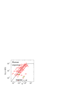
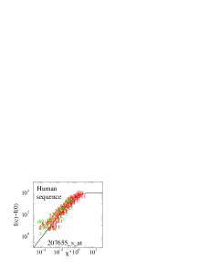
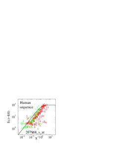
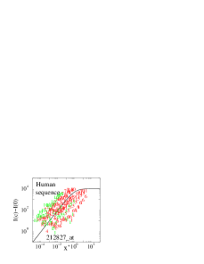
Figure 8: Collapse plots for Human sequences of the HGU133 spike-in set (part 2). The probes which are complementary to targets which the largest folding free energies are emphasized (see Table 3). They correspond to probes 207641_at5 and 209354_at8.

VI Determination of the expression level

The model defined by Eqs. (1) and (2), once all parameters have been fixed, can be used to fit the concentration $c$ starting from the measured intensities. The target concentration in solution is a measurement of the gene expression level and it is the quantity one wants to compute from the raw microarray data. As the concentrations in the spike-in experiments are known, we can compare the known values with the fitted ones. Figure 9 shows a plot of fitted concentration vs. spike-in concentration for the artificial sequences. We limit ourselves here to show the data for these sequences, but the trend is quite general and valid for other genes as well. The solid line in Fig. 9 corresponds to a line $y=x$, which means perfect agreement between spike-in and fitted values. The two other lines correspond to $y=2x$ and $y=x/2$, drawn as a guide to the eye.

As shown in Fig. 9, most of the data fall in the range between the two lines, except for the spikes TagA and TagF which give a much lower fitted concentration. All the points follow approximately straight lines with slope 1, except for the highest spike-in concentrations, corresponding to $256$ and $512$ pM. This is due to the fact that at high concentrations many probes are very close to saturation.

We note also that the fitted concentrations are all systematically lower than the spike-in values, as most of the concentrations fall in the interval $[c_{\rm spike-in}/2,c_{\rm spike-in}]$. This is a consequence of our choice to use the fitting parameters which we took from a previous study Carlon and Heim (2006) of spike-in experiments on the HGU95. We have chosen not to refit these parameters here again for HGU133, to illustrate their universal validity. The slight underestimation of the absolute concentration is not a problem, since in gene expression measurements one is only interested in fold-variations of expression levels between different experimental conditions. The fact that the data of Fig. 9 follow lines with a slope of approximately one guarantees that the fold-change in concentration in different experiments is correctly estimated.

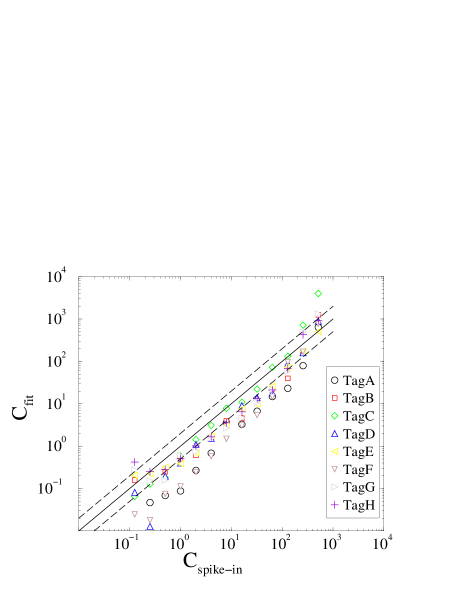
Figure 9: Plot of the fitted target concentration as a function of the spike-in concentration for the artificial sequences. The solid line correspond to the diagonal $y=x$, while the two dotted lines are $y=x/2$ and $y=2x$ and are drawn as guides to the eye. We note a systematic shift of the estimated absolute concentration compared to the spike-in one, although the fold-variations of the concentrations are correctly estimated as the majority of the data follow lines parallel to the diagonal in the plot.

Table 3: Minimal folding free energies for the targets (assumed to be 25-mers) complementary to the probes forming the spike-in HGU133 data set. These free energies are calculated with the program RNAfold.

Probe set	Probe number	-$\Delta G_{\rm fold}$(kcal/mol)
204513_s_at	4	8.70
207641_at	5	8.16
204430_s_at	10	7.79
209354_at	8	7.67
207540_s_at	10	7.45
AFFX-r2-TagA_at	1	6.52
205398_s_at	1	6.43
AFFX-PheX-3_at	10	6.18
204836_at	10	6.17
203508_at	2	6.10
206060_s_at	3	6.05

VII One cause of outliers: Target secondary structures

It is well-known that single stranded nucleic acids, particularly RNA, tend to form stable folded conformations by binding of complementary bases. Currently, algorithms that calculate RNA secondary structures are to be trusted for sufficiently short molecules, say less than 50 nucleotides, which is the situation of Affymetrix microarrays, where RNA targets are fragmented before hybridization. The average target length is $50$, but probably only shorter fragment contribute to hybridization.

We used the Vienna package Hofacker (2003) for the calculation of folded RNA structures that may form in solution and impede hybridization. We considered first 25-mer targets in solution exactly complementary to the probes of the HGU133 spike-in data set. Table 3 shows a list of probes in this set, whose complementary target has the lowest folding free energy, i.e. that of the most stable conformation, calculated at the experimental temperature of $45^{\circ}$ C. Given a folding free energy $\Delta G_{\rm fold}$, one can use the two state model approximation to find $p_{\rm fold}$ the probability that the sequence is folded into the most stable conformation:

$$p_{\rm fold}=\frac{e^{-\Delta G_{\rm fold}/RT}}{1+e^{-\Delta G_{\rm fold}/RT}}$$ (12)

where we use $T=45^{\circ}$ C. According to this expression for a folding free energy $\Delta G_{\rm fold}=-8$ kcal/mol one finds $1-p_{\rm fold}\approx 4\cdot 10^{-6}$ and $\Delta G_{\rm fold}=-6$ kcal/mol $1-p_{\rm fold}\approx 10^{-4}$. Therefore the large majority of the targets complementary to the probes listed in Table 3 are folded and not expected to participate to hybridization.

Figure 10 shows the folding configurations for the four targets with the lowest free energy of Table 3. As shown in Figs. 7 and 8 the corresponding probes have a signal which is few order of magnitude lower than that expected from the Langmuir model, although not as low as derived from Eq. (12), using the $\Delta G_{\rm fold}$ listed in Table 3. For instance, from the measured signals we find an intensity lower by a factor $10^{3}$ for the probe 204513_s_at4, instead of a factor $10^{6}$ as deduced from Eq. (12). This difference could have several origins. First, the hybridization in solution described by the term $\alpha$ in Eq. (2) may already take into account some secondary structure formation. Second, the RNA in solution is present with sequences of all lengths. The free energies listed in Table 3 refer to 25-mers, so shorter sequences will have lower folding probability than that deduced from Eq. (12) on the basis of the free energies of 25-mers. Third, even if some secondary structure is present, hybridization with the surface-bound probes is still possible if the folded configuration has some dangling ends from which binding can initiate.

We have analyzed the folding free energies of 25-mers complementary to all the probes in the HGU spike-in set. We found that about $50\%$ of the targets have folding free energy lower than $1$ kcal/mol, so that secondary structure formation can be safely neglected. About $10\%$ of the targets have a folding free energy higher than $4$ kcal/mol, so that for this fraction the secondary structure formation may interfere with the target-probe hybridization.

Summarizing, the correct estimate of the folding probability involves a complex calculation over fragments of all lengths, possibly including sequences neighboring the 25-mer part complementary to the probe. However the folding is expected to have a relevant effect for at most $10\%$ of the probes. A possible way out is that of excluding from the analysis of the gene expression levels those probes whose 25-mers folding free energy is above a certain threshold.

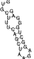
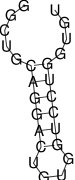
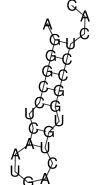
Figure 10: Folding configurations for the four targets with the lowest free energy. From left to right: 204513_s_at4, 207641_at5, 204430_s_at10 and 209354_at8.

VIII Conclusion

In this paper we have extended a previous study Carlon and Heim (2006) of Affymetrix spike-in experiments on the chip HGU95, to a novel HGU133 chipset. We used the model introduced in Ref. Carlon and Heim (2006) which takes into account both target-probe and target-target hybridization in solution. The hybridization free energies are calculated from the nearest-neighbor model Bloomfield et al. (2000) using the experimental parameters for RNA/DNA Sugimoto et al. (1995, 2000) and RNA/RNA Xia et al. (1998). There are four global fitting parameters in the model that we took from Ref. Carlon and Heim (2006). We found that these parameters fit well also the current data on the HGU133 chipset, apart for a systematic small shift of all the estimates of the absolute target concentrations.

There are several features that make the spike-in data of the more recent HGU133 chip interesting. First of all the spike-in set contains a larger number of sequences compared to the HGU95 experiments (42 instead of 14) and the chip has been entirely redesigned. Secondly, the spike-in sequences contain some of artificial origin, designed to avoid any cross hybridization with human RNAs, but prepared and labeled exactly as all other spikes. We find that these artificial sequences fit best the hybridization model, as they show the best collapses when the data are rescaled and plotted as function of an appropriate thermodynamic variable. The good agreement suggests indeed that the simple model describes rather well the hybridization in Affymetrix arrays and that the deviations observed for some human sequences are probably related to the non-optimal design of the sequences for a given probe.

When compared to the human sequences of the HGU95 spike-in experiments analyzed in Ref. Carlon and Heim (2006), we find that the artificial spikes of the HGU133 set show definitely better collapses. However, when comparing the human sequences of the HGU133 with those in the HGU95 experiment we find on average a better collapse for the latter. Only few probes out of the 32 human spikes of the HGU133 experiment have a better collapse than those of the HGU95.

Interestingly, the physics-based modeling developed here allows to assign to each probe set a quality score based on the level of agreement on the Langmuir model. This information may be used to reconsider and eventually redesign the probe sets of low quality.

Finally, we have discussed the physical basis of hybridization in solution and of RNA secondary structure formation. The latter effect, according to the statistics over the spike-in probes, will be relevant for about 10% of the probes only. The sequences with the highest folding probability correspond to probes whose measured fluorescent intensities is well-below that predicted from the Langmuir model.

According to our current understanding of the system (see also Refs. Carlon and Heim (2006); Heim et al. (2006)), the hybridization in solution of partially complementary RNA molecules has a strong influence. One of the reasons for that is that RNA/RNA interaction parameters are, at given temperature and salt concentration, stronger than the DNA/DNA or RNA/DNA parameters. The simple approximation given in Eq.(2) captures the major features of the hybridization in solution. However, an improvement over this approach, as discussed above, remains an open challenge.

We acknowledge financial support from the Van Gogh Programme d’Actions Intégrées (PAI) 08505PB of the French Ministry of Foreign Affairs and the NWO grant 62403735.

References

- Schena et al. (1995) M. Schena, D. Shalon, R. W. Davis, and P. O. Brown, Science 270, 467 (1995).
- Marshall (2004) E. Marshall, Science 306, 630 (2004).
- Tan et al. (2003) P. K. Tan et al., Nucleic Acids Res. 31, 5676 (2003).
- Peterson et al. (2002) A. W. Peterson, L. K. Wolf, and R. M. Georgiadis, J. Am. Chem. Soc. 124, 14601 (2002).
- Okahata et al. (1998) Y. Okahata et al., Anal. Chem. 70, 1288 (1998).
- Vainrub and Pettitt (2002) A. Vainrub and B. M. Pettitt, Phys. Rev. E 66, 041905 (2002).
- Held et al. (2003) G. A. Held, G. Grinstein, and Y. Tu, Proc. Natl. Acad. Sci. 100, 7575 (2003).
- Naef and Magnasco (2003) F. Naef and M. O. Magnasco, Phys. Rev. E 68, 011906 (2003).
- Hagan and Chakraborty (2004) M. F. Hagan and A. K. Chakraborty, J. Chem. Phys. 120, 4958 (2004).
- Halperin et al. (2004) A. Halperin, A. Buhot, and E. B. Zhulina, Biophys. J. 86, 718 (2004).
- Binder and Preibisch (2005) H. Binder and S. Preibisch, Biophys. J. 89, 337 (2005).
- Carlon and Heim (2006) E. Carlon and T. Heim, Physica A 362, 433 (2006).
- Sugimoto et al. (1995) N. Sugimoto et al., Biochemistry 34, 11211 (1995).
- Sugimoto et al. (2000) N. Sugimoto, M. Nakano, and S. Nakano, Biochemistry 39, 11270 (2000).
- Xia et al. (1998) T. Xia et al., Biochemistry 37, 14719 (1998).
- Heim et al. (2006) T. Heim, J. Klein Wolterink, E. Carlon, and G. T. Barkema, J. Phys.: Cond. Matt. 18, S525 (2006).
- Bloomfield et al. (2000) V. A. Bloomfield, D. M. Crothers, and I. Tinoco, Jr., Nucleic Acids Structures, Properties and Functions (University Science Books, Mill Valley, 2000).
- (18) C. J. Burden and Y. Pittelkow and S. R. Wilson, “An adsorption model of hybridization behaviour on oligonucleotide microarrays”, preprint q-bio.BM/0411005.
- (19) Affymetrix Europe, private communication.
- Hofacker (2003) I. L. Hofacker, Nucleic Acids Res. 31, 3429 (2003).