Structure and function of negative feedback loops at the interface of genetic and metabolic networks

1 abstract

The molecular network in an organism consists of transcription/translation regulation, protein-protein interactions/modifications and a metabolic network, together forming a system that allows the cell to respond sensibly to the multiple signal molecules that exist in its environment. A key part of this overall system of molecular regulation is therefore the interface between the genetic and the metabolic network. A motif that occurs very often at this interface is a negative feedback loop used to regulate the level of the signal molecules. In this work we use mathematical models to investigate the steady state and dynamical behaviour of different negative feedback loops. We show, in particular, that feedback loops where the signal molecule does not cause the dissociation of the transcription factor from the DNA respond faster than loops where the molecule acts by sequestering transcription factors off the DNA. We use three examples, the bet, mer and lac systems in E. coli, to illustrate the behaviour of such feedback loops.

2 Introduction

Gene expression in bacterial cells is modulated to enhance the cell’s performance in changing environmental conditions. To this end, transcription regulatory networks continuously sense a set of signals and perform computations to adjust the gene expression profile of the cell. A subset of such signals contains molecules that the cell can metabolize. These molecules range from nutrients to toxic compounds. A commonly occurring motif in the networks sensing such signal molecules is a negative feedback loop.  In this motif an enzyme used to metabolize the signal molecule is controlled by a regulator whose action, in turn, is regulated by the same signal molecule. This motif allows for genes that are not transcription factors to negatively regulate their own synthesis.

Because these negative feedback loops are situated at the interface of genetic [1, 2] and metabolic [2, 3] networks, understanding their behavior is crucial for building integrated network models, as well as synthetic gene circuits [4, 5, 6]. In fact, if one ignores the interface, the network topology gives the impression that feed back mechanisms are less frequent than feed forward loops [7, 8]. In addition, by ignoring feedback associated to signal molecules one would also tend to overemphasize the modular features of the overall system [9] and underemphasize the average number of incoming links to proteins.

Even within the framework of a negative feedback loop there are several different mechanisms possible both for transcriptional regulation and for the action of the signal molecule. We list below four mechanisms which are present in living cells, with examples taken from E. coli (Fig. 1):

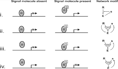
Figure 1: Schematic diagrams of four types of negative feedback loops containing proteins and signal molecules. Regulation of the promoter (arrow) transcribing the enzyme (E) that can metabolize the signal molecule (s) is shown in the first two columns. R represents the regulator. A network representation of each regulation mechanism is shown in the rightmost column. This is not a complete logical list of all combinatorial possibilities, it includes only the ones where real examples have been found.

(i) The regulator, R, represses the transcription of the enzyme, E, which metabolizes the signal molecule, s. The signal molecule binds to the repressor resulting in the dissociation of the R-operator complex and an increase in the production of E. This mechanism is exemplified by a negative feedback loop in the lac system [10], where the roles of R, E and s are played by LacI, $\beta$-galactosidase, and lactose, respectively.

(ii) R represses the transcription of E which metabolizes s. But here the signal molecule can bind to R even when it is at the operator site. When this happens the effect of R on the promoter activity is cancelled, or even reversed. Two examples of this kind are the bet [11, 12] and mer [13] systems, which are involved in the response of cells to the harmful conditions of osmotic stress and presence of mercury ions, respectively.

(iii) Here the regulator, R, is an activator of the transcription of E when s is bound to it. Without the signal molecule, R cannot bind to the DNA site and activate transcription. For instance, MalT in complex with maltose is a transcriptional activator of genes which metabolize maltose. This mechanism differs from (ii) in that in the absence of s, R is a repressor in (ii) while here it does not affect the promoter activity.

(iv) Here too, R alone cannot bind to the operator site. However, in contrast to (iii), R bound to s represses the transcription of E. Further, in this case E increases the production of the signal molecule, rather than metabolizing it, thereby again making the overall feedback negative. One such example is the regulation of de novo purine nucleotide biosynthesis by PurR [14, 15].

A major difference between these four loops is the manner in which the signal molecule acts. In (i) the binding of s to R drastically reduces its affinity to the DNA site. On the other hand, in (ii), (iii) and (iv), the signal molecule increases, or does not significantly alter, the binding affinity of R and can also affect the action of the regulator when it is bound to the DNA. Henceforth we will refer to these two methods of action as ‘mechanism (1)’ and ‘mechanism (2)’.

In this paper we have investigated how this difference in the mechanism of action of the signal molecule translates to differences in the steady state and dynamical behaviour of the simplest kind of negative feedback loops containing proteins and signal molecules. These loops have only one step, E, between the regulator and the signal molecule. Further, the regulator is assumed to have only one binding site on the DNA. We concentrate on the cases where R is a repressor and s lifts the repression (i and ii). In particular, we show that the two mechanisms differ substantially in their dynamic behaviour when R is large enough to fully repress the promoter of E in the absence of s. We illustrate how the difference is used in cells by the examples of the bet, mer and lac systems.

3 Results

3.1 Steady state behaviour of feedback loops

First we consider how the steady state activity of the promoter of E responds to changes in the concentration of s for each of the mechanisms.

Consider a feedback loop, like Fig. 1 (i), where the operator can be found in one of two states: free, $O_{\rm free}$, and bound to the regulator, $(RO)$, with the total concentration of operator sites being a constant: $O_{\rm tot}=O_{free}+(RO)$. We assume that the promoter is active only when the operator is free, and completely repressed when it is bound by R. This loop uses mechanism (1) and is an idealization of the lac system in E. coli. The promoter activity is given by:

$$A_{1}=\frac{O_{\rm free}}{O_{\rm tot}}=\frac{O_{\rm free}}{O_{\rm free}+(RO)}.$$ (1)

In steady state, $O_{\rm free}$ and $(RO)$ can be expressed as functions of the total concentration of regulators, $R_{\rm tot}$, and the concentration of signal molecules, $s$. The expression also contains the parameters $K_{RO}$ and $h$ (the equilibrium binding constant for R-operator binding and the corresponding Hill coefficient), $K_{Rs}$ and $h_{s}$ (for R-s binding.) Equation 6 in the Methods section contains all the details. The main effect of s is to decrease the amount of free R because $R_{\rm tot}=R_{\rm free}+(Rs)$, where $(Rs)$ is the concentration of the R-s complex.

For a feedback loop using mechanism (2), the operator can be found in one of three states: free, $O_{\rm free}$, bound to the regulator, $(RO)$, and bound to the regulator along with the signal molecule, $(RsO)$. The total concentration of operator sites, $O_{\rm tot}=O_{free}+(RO)+(RsO)$, is constant. The promoter activity has a basal value (normalized to 1) when the operator is free. When the regulator alone is bound it represses the activity. We assume the activity in this state is zero. When the operator is bound by R along with s the activity returns to the basal level. This is an idealization of the bet system. Here, the promoter activity is given by:

$$A_{2}=\frac{O_{\rm free}+(RsO)}{O_{\rm free}+(RO)+(RsO)}.$$ (2)

The main effect of s comes from the second term in the numerator of equation 2, which is the concentration of the R-s-operator complex. As in the case of $A_{1}$, in steady state the activity can be expressed in terms of $R_{\rm tot}$ and $s$. Because of the third state of the operator, $(RsO)$, the expression for $A_{2}$ includes one more parameter, $K_{RsO}$, the equilibirum binding constant for R-operator binding when s is bound to R (see equation 8 in the Methods section for details.)

For mechanism (2), we mainly consider the case where $K_{RsO}=K_{RO}$, i.e., the binding of the signal molecule does not change the binding affinity of the regulator to the operator. This is the simplest situation and illustrates the basic differences between the two mechanisms. In real systems these binding constants are often different. However, as we show, for bet and mer the inequality of $K_{RsO}$ and $K_{RO}$ does not obscure the differences caused by the two mechanisms of action of the signal molecule. This is because the main effect of changing $K_{RsO}$ is simply to shift the position of the response curve. Only when $K_{RsO}$ becomes very large (which results in dissociation of R from the operator when s binds to it, as in lac) does mechanism (2) effectively reduce to mechanism (1).

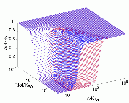
Figure 2: Promoter activities for the two mechanisms as a function of $R_{\rm tot}$ and $s$. Red: $A_{1}$ (equation 1 and 6); Blue: $A_{2}$ (equation 2 and 8.) Parameter values (see equations 6 and 8) are: $K_{RO}=1,K_{Rs}=100,h=2,h_{s}=1$ and $K_{RsO}=1$ for mechanism (2). Choosing $h=2$ assumes that two protein subunits are involved in the R-operator binding.

Figure 2 shows the activities $A_{1}$ and $A_{2}$ for a range of values of $R_{\rm tot}$ and $s$. The following observations can be made from the figure:

• For sufficiently small values of $R_{\rm tot}$ there is no difference between $A_{1}$ and $A_{2}$.

• From $R_{\rm tot}/K_{RO}=1$ and higher, $A_{1}$ requires larger and larger s to rise to its maximum value, i.e., its effective binding constant $K_{\rm eff}$ increases with $R_{\rm tot}$ (where we define $K_{\rm eff}$ to be the value of $s$ at which the activity is half-maximum.)

• $A_{2}$, on the other hand, has a $K_{\rm eff}$ which is remarkably robust to changes in $R_{\rm tot}$, remaining close to $K_{Rs}$ for $R_{\rm tot}/K_{RO}>1$.

• Zooming in to the low $s$ region shows that $A_{2}$ rises more steeply than $A_{1}$ for small $s$ values.

All these features can be explained by taking a closer look at the equations for $A_{1}$ (eq. 1 and 6) and $A_{2}$ (eq. 2 and 8.) Taking the observations in reverse order, first we see that for small values of $s$, the promoter activities rise as a power of $s$: $A(s)\approx A(0)+{\rm const.}\times s^{a}$. From equations 6 and 8 we find that this power $a=h_{s}$ for mechanism (1) and $a=h\times h_{s}$ for mechanism (2). Thus, as long as $h>1$, mechanism (2) will have a steeper response at small values of $s$.

Next, let us consider the amount of inducer $\;s=K_{\rm eff}$ needed to half-activate the promoter under the two mechanisms. The fact that $K_{\rm eff}$ is close to $K_{Rs}$ for $A_{2}$ is because of the term $(RsO)$, which occurs in both the numerator and the denominator of equation 2. When $R_{\rm tot}$ is large enough (i.e., $R_{\rm tot}>K_{R0}$), the operator is rarely free, and the constant term (=1) in eq. 8 can be disregarded from both numerator and denominator. In that case $A_{2}$ only depends on the ratio between the binding affinities $K_{RsO}/K_{RO}$. Accordingly $A_{2}$ becomes independent of the value of $R_{tot}$ for $R_{tot}>K_{RO}=1$.

On the other hand, the activity $A_{1}$ is always highly dependent on $R_{tot}$. From equation 6 we see that $A_{1}$ reaches half-maximum when $(RO)=O_{\rm free}$. This happens when $(s/K_{Rs})^{h_{s}}\approx(R_{\rm tot}/K_{RO})$. Therefore $K_{\rm eff}$ is an increasing function of $R_{\rm tot}$ for mechanism (1).

For both mechanisms, when $R_{\rm tot}$ drops below $min(K_{RsO},K_{RO})$ we enter a regime where the inducer is not needed for derepression. For our standard parameters, repressor concentration $R_{\rm tot}<K_{RO}$ implies that $O_{\rm free}$ and $(RO)$ dominate $(RsO)$ in equation 2. Thereby the functional form of the activity $A_{2}$ approaches that of $A_{1}$, as indeed seen from the $R_{\rm tot}/K_{RO}<1$ regime in Fig. 2.

In addition to these mathematical arguments, the above observations can be understood physically from the nature of the processes allowed in mechanisms (1) and (2). Consider the case of a fully repressed promoter (when $R_{\rm tot}\gg K_{RO}$). Mechanism (1) then requires dissociation of $R$ from the operator for the activity to rise and this is associated with a free energy cost proportional to ${\rm ln}(R_{\rm tot}/K_{RO})$. In mechanism (2) there is no such cost and therefore a smaller amount of $s$ is required to achieve the same level of inhibition of R. Thus, for genes which are typically completely repressed, and transcription of which, on the other hand, may be needed suddenly, mechanism (1) is inferior to mechanism (2) because it needs a larger amount of $s$. After first discussing three real systems, we will elaborate on this response advantage by comparing the explicit time dependence of the two mechanisms in the next section.

The most general framework within which the promoter activities of the enzymes in the bet, mer and lac systems can be represented is the following generalization of equations 1 and 2:

$$A=\frac{\alpha O_{\rm free}+\beta(RO)+\gamma(RsO)}{O_{\rm free}+(RO)+(RsO)}.$$ (3)

Equation 9 in the Methods section shows the dependence of $A$ on $R_{\rm tot}$ and $s$. $\alpha,\beta,\gamma$ are constants dependent on which system we are trying to describe. $\alpha$ is the promoter activity in the absence of R and is used as a reference (1.00). $\beta$ and $\gamma$ are the relative promoter activities in the presence of R alone, and R together with s, respectively. Table 1 shows the values of $\alpha,\beta,\gamma$ as well as how the binding affinity of R to the operator is changed by the binding of s (the ratio $K_{RsO}/K_{RO}$) for the three systems. We have used the Hill coefficients $h=2$ (assuming that two protein subunits are involved in DNA binding) and $h_{s}=1$ (for simplicity and to compare with Fig. 2.) Mechanism (1) and (2) are special cases of this equation. Equations 1 and 6, for mechanism (1), are obtained by setting $\alpha=1,\;\beta=0$ and taking the limit $K_{RsO}\rightarrow\infty$ (the value of $\gamma$ is irrelevant in this limit). Equations 2 and 8, for mechanism (2), are obtained by setting $\alpha=1,\;\beta=0,\;\gamma=1$. From Table 1, it is clear then that lac uses mechanism (1) and bet uses mechanism (2). mer is an even more extreme case of mechanism (2) where the $(RsO)$ term has a much larger weight ($\gamma\gg 1$) than the idealized mechanism (2).

System	$\alpha$	$\beta$	$\gamma$	$K_{RsO}/K_{RO}$	References
bet	1	0.32	0.83	0.29	[11, 12]
mer	1	0.13	13.71	3.5	[13]
lac	1	0.06	1	1000	[16, 17]

Table 1: Values of parameters in equation 3 for three systems found in E. coli. In the case of lac we used a simplified case, where the lac promoter is repressed by LacI binding to a single operator, O1.

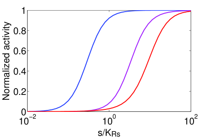
Figure 3: Promoter activity, $A$, (see equation 3 and 9) versus $s$ for the bet (blue), mer (purple), lac (red) systems in E. coli. Because the promoter activities for the three systems have different minimum and maximum values, for easier comparison we have plotted $(A-A_{\rm min})/(A_{\rm max}-A_{\rm min})$, where $A_{\rm min}=A(s=0)$ and $A_{\rm max}=A(s=\infty)$. In all cases, we kept $R_{tot}/K_{RO}=10$.

Fig. 3 shows the response curves for the bet, mer and lac systems. bet and mer, representatives of mechanism (2), and lac, a representative of mechanism (1), indeed behave similar to the idealized versions of the two mechanisms investigated in Fig. 2. The difference between bet and mer is the result of changes in the binding affinity of R in the absence and presence of s.

A further complication that could occur in real systems is that the probabilities of RNA polymerase recruitment could be different for different states of the operator. We find that taking the changing probabilities of RNA polymerase recruitment into account does not change the mathematical form of the equations for the promoter activities (see Methods.) Thus, this additional complication does not affect our results.

3.2 Dynamical behaviour of feedback loops

We now turn to an analysis of differences in the temporal behaviour of the feedback mechanisms. We model the dynamics by two coupled differential equations:

$$\frac{dE}{dt}=A(R_{\rm tot},s)-E$$

and

$$\frac{ds}{dt}=c-kEs.$$

$E$ and $s$ represent the concentrations of the enzyme and signal molecule, respectively. The first term in the $dE/dt$ equation is the rate of production of E which is equal to the promoter activity, $A$ (equations 3 and 9). The second term represents degradation of E. The second equation describes the evolution of the concentration of s; it increases if there is a source, $c>0$, of s (for instance from outside the cell) and decreases due to the action of the enzyme E. In the first equation both terms could be multiplied by rate constants, representing the rates of transcription, translation and degradation. However, we have eliminated these constants by measuring time, $t$, in units of the degradation time of E, and by rescaling $E$ appropriately (see the Methods section for details.) Thus, in these equations, $E$ and $t$ are dimensionless, with $E$ lying between 0 and 1. $k$ can then be interpreted as the maximum rate of degradation of s in units of the degradation rate of E.

a.

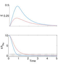
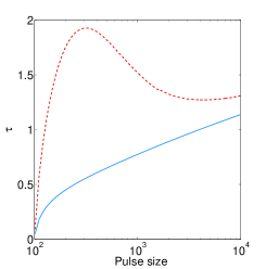
b.

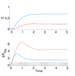
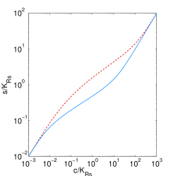
Figure 4: a. Left panel: time course for levels of E and s when there is no source of s ($c=0$) and the system is subject to an instantaneous pulse lifting the value of $s$ from zero to $10\times K_{Rs}$ at time $t=0$. The shaded region corresponds to $s<K_{Rs}$. Right panel: the time (after the pulse), $\tau$, required for each mechanism to reduce the value of $s$ down to $K_{Rs}$, for different sizes of the initial pulse. b. Left panel: time course of levels of E and s when a source of s ($c=10\times K_{Rs}$ per degradation time of E) is suddenly introduced at time $t=0$. Right panel: Difference between the steady state values of $s$ for the two mechanisms as a function of the value of the source term, $c$. In all plots the red, dashed line indicates mechanism (1) and the blue, solid line, mechanism (2). Parameter values are: $K_{RO}=1,K_{Rs}=100,h=2,h_{s}=1,k=10$, and $K_{RsO}=1$ for mechanism (2). The active degradation rate $k$ has been chosen to be much larger than the degradation rate of E (which is unity).

Fig. 4a (left panel) shows what happens if the cell is subject to a sudden pulse of s. That is, the source $c=0$ always, but at time $t=0$ the concentration of s abruptly jumps from zero to $10\times K_{Rs}$. This triggers an increase in the production of E which then starts to decrease the concentration of s. There is no further addition of s to the system, so eventually all of it is removed and the system returns to its condition before the pulse. From the figure we see that, for the same parameter values, mechanism (2) results in a much faster removal of s because the response of E to the pulse is larger. The right panel adds further evidence to this conclusion. It shows, for both mechanisms, perturbed by varying sized pulses of s, the time taken for the concentration of s to fall to $K_{Rs}$. This measure shows that mechanism (2) generally responds faster than mechanism (1). The two mechanisms converge for small perturbations because there is no signal to respond to (levels of $s$ are very low), and for very large perturbations because then the promoter becomes fully activated by the huge concentration of the inducing molecule s.

Fig. 4b shows what happens when the cell is subject to the appearance of a constant source of s. At time $t=0$ the value of $c$ abruptly jumps from zero to $10\times K_{Rs}$ per degradation time of E. In response, the production of E is increased and eventually reaches a new steady state value to deal with the constant influx of s (left panel). From the right panel of the figure it is evident that mechanism (2) is able to suppress the amount of s much more than mechanism (1) for most values of the rate of influx. Again, for similar reasons, the two mechanisms converge at small and large values of $c$.

These observations apply for the case when $K_{RsO}=K_{RO}$ for mechanism (2). The only effect on the dynamical equations caused by changing the ratio $K_{RsO}/K_{RO}$ lies in the expression for $A$ in the first term of the $dE/dt$ equation. As mentioned in the previous section, changing this ratio mainly results in shifting of the response curve and as $K_{RsO}$ is increased, $A_{2}$ approaches $A_{1}$. For the dynamics this results in an increase in $\tau$ (for a pulse) and in the steady state value of $s$ (for a source) as $K_{RsO}/K_{RO}$ is increased. These values approach those for mechanism (1) in the limit $K_{RsO}/K_{RO}\rightarrow\infty$. The amount by which $K_{RsO}$ has to be boosted to effectively reduce mechanism (2) to mechanism (1) increases with increasing $R_{\rm tot}$, as in the steady state case.

4 Discussion

In the present paper we have discussed various strategies for negative feedback mechanisms involving the action of one signal molecule on a transcription factor. In particular, we have investigated two broadly different ways in which the signal molecule may change the action of the transcription factor: first, it could inhibit its action by sequestering it, and second, it could bind to the transcription factor while it is on the DNA site and there alter its action. The first mechanism occurs when the binding of the signal molecule reduces the affinity of the transcription factor to such an extent that it cannot subsequently remain bound to the DNA. This kind of inhibition of the transcription factor occurs in the lac system, where (allo)lactose reduces the binding affinity of LacI to the operator O1 by a factor of 1000 [17]. This mechanism has also been exploited in synthetic gene networks [4, 5]. In the second mechanism the binding affinity is not altered that much; bet and mer belong to this category. In the case of mer the presence of the signal molecule reverses the action of the transcription factor, changing it from a repressor to an activator [13].

In steady state, the two mechanisms differ most when the levels of the transcription factor are large enough to ensure substantial repression in the absence of the signal molecule. The underlying reason for these differences is that, in this regime of full repression, for each transcription factor that binds to the signal molecule there is, for mechanism (1), an extra energy cost for the dissociation of the transcription factor from the DNA. The dynamical behaviour of feedback loops based on mechanisms (1) and (2) also differ substantially when promoters are in the fully repressed regime. We have shown that when the systems are perturbed by the sudden appearance of either a pulse or a source of signal molecules, mechanism (2) is generally faster and more efficient than mechanism (1) in suppressing the levels of the molecule. This prediction could be tested using synthetic gene circuits which implement these two mechanisms, for instance by extending the circuits built in ref. [6]. In addition, this observation fits neatly with the fact that the bet and mer systems use versions of mechanism (2), because they respond to harmful conditions (osmotic stress and the presence of mercury ions, respectively) and therefore need to respond quickly, while mechanism (1) is associated with lac, a system involved in metabolism of food molecules which therefore does not need to be as sensitive to the concentration of the signal molecules. In the case of lac it is probably energetically disadvantageous for the cell to respond to low levels of lactose sources [18].

The differences between mechanisms are clear when they are compared keeping all parameters constant. In cells, however, parameter values vary widely from one system to another which can obscure the differences caused by the two mechanisms. For instance, it is possible to increase the speed of response of mechanism (1) by reducing the $K_{Rs}$ value (i.e., increasing the binding strength between the regulator and the signal molecule.) Keeping all other parameters constant $K_{Rs}$ needs to be decreased by a factor 10 for mechanism (1) to behave the same as mechanism (2) when $R_{\rm tot}=10\times K_{RO}$. This factor increases as $R_{\rm tot}$ increases, i.e., as the repression is more complete. This can again be understood in terms of the extra energy cost for mechanism (1): increasing $K_{Rs}$ sufficiently makes the extra energy cost insignificant compared to the R-s binding energy. Thus, a negative feedback loop in a real cell which needs to respond to signals on a given fast timescale could do so either by using mechanism (2), or by using mechanism (1) with a substantially larger R-s binding affinity. For signal molecules where it is not possible for the R-s binding to be arbitrarily strengthened, mechanism (2) would be the better choice. On the other hand, mechanism (2) also has its disadvantages. For instance, at promoters with complex regulation the DNA bound transcription factor using mechanism (2) may interfere with the action of other transcription factors.

In Figure 1 we showed 4 examples, and have extensively discussed example (i) and (ii). Another implementation of mechanism (2) is example (iii), with an activity $A_{3}=(RsO)/[O_{\rm free}+(RsO)]$. In general this regulatory module is at least as efficient as mechanism (2), with a dynamical response which is even more efficient in the intermediate range of $s$ (around $K_{Rs}$). The loop in Fig. 1(iv) is, on the other hand, a different kind of negative feedback from the other three examples. It involves synthesis of the signal molecule, and thus is aimed at maintaining a certain concentration of the molecule, rather then minimising or consuming it. In practice, it is the kind of feedback that is common in biosynthesis pathways, where it helps maintain a certain level of amino acids, nucleotides, etc., inside the cell.

The simple one-step, single-operator negative feedback loops investigated here clearly indicate that the mechanism of action of the signal molecule is a major determinant of the steady state and dynamical behaviour of the loop. Additional complexity in the mechanism of regulation (e.g., cooperative binding of a transcription factor to multiple binding sites) or of the regulatory region (competing transcription factors or multiple regulators responding to different signals) [19, 20] would open up more avenues for the differences between the two mechanisms to manifest themselves.

These feedback loops form the link connecting the genetic and metabolic networks in cells. In fact, such loops involving signal molecules are likely to be a dominant mechanism of feedback regulation of transcription. Feedback using only regulatory proteins, without signal molecules, is probably too slow because it relies on transcription to change the levels of the proteins. Negative auto-regulation can speed up the response of transcription regulation [21]. Nevertheless, feedback loops based on translation regulation [22, 23], active protein degradation [24, 25] or metabolism of signal molecules will certainly be able to operate on much faster timescales. This is probably why feedback loops are rare in purely transciptional networks, which has contributed to the view that feed forward loops are dominant motifs in transcription regulation. Taking feedback loops involving signal molecules into account alters this viewpoint substantially. In E. coli the number of feedforward loops in the transcription regulatory network has been reported to be 40 [7, 8]. Based on data in the EcoCyc database [2], we know that there are more than 40 negative feedback loops involving signal molecules where the regulation is by a transcription factor. Adding this many feedback loops to the genetic network would also change the network topology substantially. In particular, it would diminish the distinction between portions of the network that are downstream and upstream of a given protein. The effect of this would be to make the network more interconnected and reduce the modularity of the network by increasing the number of links between apparently separate modules.

5 Methods

5.1 Promoter activity for mechanism (1)

The operator can exist in one of two states: (i) free, $O_{\rm free}$, and (ii) bound to the regulator, $(RO)$. If the concentration of free regulators is $R_{\rm free}$ then

$$(RO)=\left(\frac{R_{\rm free}}{K_{RO}}\right)^{h}O_{\rm free}.$$

Similarly, the concentration of regulators bound to signal molecules is

$$(Rs)=\left(\frac{s}{K_{Rs}}\right)^{h_{s}}R$$

and the total concentration of regulators, a constant, is given by

$$R_{\rm tot}=R_{\rm free}+(RO)+(Rs).$$

We assume that the number of signal molecules is much larger than the number of regulators which, in turn, is much larger than the number of operator sites, i.e., $s\gg R_{\rm tot}\gg O_{\rm tot}$. Then we can take $s$ to be approximately constant and we can take $(RO)\ll(Rs)$, giving:

$$R_{\rm tot}=R_{\rm free}+\left(\frac{s}{K_{Rs}}\right)^{h_{s}}R_{\rm free},$$

$$\Rightarrow R_{\rm free}=\frac{R_{\rm tot}}{1+(s/K_{Rs})^{h_{s}}}$$ (4)

and

$$(RO)=\left[\frac{(R_{\rm tot}/K_{RO})}{1+(s/K_{Rs})^{h_{s}}}\right]^{h}O_{\rm free}$$ (5)

Using these and $O_{\rm tot}=O_{\rm free}+(RO),$ we get:

$$A_{1}\equiv\frac{O_{\rm free}}{O_{\rm tot}}=\frac{1}{1+\left[\frac{(R^{tot}/K_{RO})}{1+(s/K_{Rs})^{h_{s}}}\right]^{h}}.$$ (6)

5.2 Promoter activity for mechanism (2)

The operator can exist in one of three states: (i) free, $O_{\rm free}$, (ii) bound to the regulator, $(RO)$, and (iii) bound to the regulator along with the signal molecule, $(RsO)$.

Again, with similar assumptions, we get equation 4 and 5 for $R_{\rm free}$ and $(RO)$ plus an additional expression for $(RsO)$:

$$(RsO)=\left[\frac{(R_{\rm tot}/K_{RsO})(s/K_{Rs})^{h_{s}}}{1+(s/K_{Rs})^{h_{s}}}\right]^{h}O_{\rm free}.$$ (7)

Using $O_{\rm tot}=O_{\rm free}+(RO)+(RsO)$ and equation 2 for $A_{2}$, we get:

$$A_{2}=\frac{1+\left[\frac{(R^{tot}/K_{RsO})(s/K_{Rs})^{h_{s}}}{1+(s/K_{Rs})^{h_{s}}}\right]^{h}}{1+\left[\frac{(R^{tot}/K_{RO})}{1+(s/K_{Rs})^{h_{s}}}\right]^{h}+\left[\frac{(R^{tot}/K_{RsO})(s/K_{Rs})^{h_{s}}}{1+(s/K_{Rs})^{h_{s}}}\right]^{h}}.$$ (8)

5.3 General expression for promoter activity

The most general expression for the activity, shown in equation 3, can also be rewritten using the expressions for $(RO)$ and $(RsO)$ calculated above:

$$A=\frac{\alpha+\beta\left[\frac{(R^{tot}/K_{RO})}{1+(s/K_{Rs})^{h_{s}}}\right]^{h}+\gamma\left[\frac{(R^{tot}/K_{RsO})(s/K_{Rs})^{h_{s}}}{1+(s/K_{Rs})^{h_{s}}}\right]^{h}}{1+\left[\frac{(R^{tot}/K_{RO})}{1+(s/K_{Rs})^{h_{s}}}\right]^{h}+\left[\frac{(R^{tot}/K_{RsO})(s/K_{Rs})^{h_{s}}}{1+(s/K_{Rs})^{h_{s}}}\right]^{h}}.$$ (9)

5.4 Taking into account RNA polymerase recruitment

A more correct, but more cumbersome, way to calculate the promoter activities is to explicitly take RNA polymerase into account. Then, in the most general case, the system can be in one of 6 states:

• R not bound to operator, RNAP not recruited: weight=1.

• R not bound to operator, RNAP recruited: wt=$p_{1}P$.

• R bound to operator, RNAP not recruited: wt=$(RO)$.

• R bound to operator, RNAP recruited: wt=$(RO)p_{2}P$.

• R-s bound to operator, RNAP not recruited: wt=$(RsO)$.

• R-s bound to operator, RNAP recruited: wt=$(RsO)p_{3}P$.

Here $p_{1,2,3}$ are the probabilities (per concentration) for recruitment of RNA polymerase in the three different states of the operator, and $P$ is the concentration of RNA polymerase. Taking the promoter activity to be 0 when the polymerase is not recruited and $\alpha^{\prime},\beta^{\prime},\gamma^{\prime}$ in states (2), (4) and (6), respectively, the activity can be written as follows:

$$A=\frac{(p_{1}\alpha^{\prime}+p_{2}\beta^{\prime}(RO)+p_{3}\gamma^{\prime}(RsO))P}{1+p_{1}+(1+p_{2})(RO)+(1+p_{3})(RsO)}.$$

By absorbing the constants $p_{1,2,3}$ into $K_{Rs}$, $K_{RO}$ and $K_{RsO}$, we recover equation 9.

5.5 Rescaling of the dynamical equations

With all rate constants included, the dynamical equations for the time evolution of the concentrations of E and s can be written as follows:

$$\frac{dE}{dt}=k_{1}A(R_{\rm tot},s)-\gamma E,$$

$$\frac{ds}{dt}=c^{\prime}-k^{\prime}Es.$$

Now measuring time in units of the degradation time of E: $t^{\prime}=\gamma t$, and transforming E using $E^{\prime}=E(\gamma/k_{1})$, we get

$$\frac{dE^{\prime}}{dt^{\prime}}=A(R_{\rm tot},s)-E^{\prime}$$

$$\frac{ds}{dt^{\prime}}=\frac{c^{\prime}}{\gamma}-\frac{k^{\prime}k_{1}}{\gamma^{2}}E^{\prime}s$$

which, with $c\equiv c^{\prime}/\gamma$ and $k\equiv k^{\prime}k_{1}/\gamma^{2}$, are the equations used in the main text.

6 Acknowledgements

This work was supported by the Danish National Research Foundation.

REFERENCES

- [1] Salgado, H., Santos-Zavaleta, A., Gama-Castro, S., Millan-Zarate, D., Diaz-Peredo, E., Sanchez-Solano, F., Perez-Rueda, E., C. Bonavides-Martinez, C., and Collado-Vides, J. (2001) Regulondb (version 3.2): Transcriptional regulation and operon organization in escherichia coli k-12. Nucleic Acids Res., 29, 72–74.
- [2] Keseler, I., Collado-Vides, J., Gama-Castro, S., Ingraham, J., Paley, S., Paulsen, I., Peralta-Gil, M., and Karp, P. (2005) Ecocyc: A comprehensive database resource for escherichia coli. Nucleic Acids Res., 33, D334–D337.
- [3] Edwards, J. S. and Palsson, B. O. (2000) The escherichia coli mg1655 in silico metabolic genotype: Its definition, characteristics, and capabilities. Proc. Natl. Acad. Sci. (USA), 97, 5528–5533.
- [4] Gardner, T. S., Cantor, C. R., and Collins, J. J. (2000) Construction of a genetic toggle switch in escherichia coli. Nature, 403, 339–342.
- [5] Kobayashi, H., Kaern, M., Araki, M., Chung, K., Gardner, T. S., Cantor, C. R., and Collins, J. J. (2004) Programmable cells: interfacing natural and engineered gene networks. Proc. Natl. Acad. Sci. (USA), 101, 8414–8419.
- [6] Guido, N. J., Wang, X., Adalsteinsson, D., McMillen, D., Hasty, J., Cantor, C. R., Elston, T. C., and Collins, J. J. (2006) A bottom-up approach to gene regulation. Nature, 439, 856–860.
- [7] Shen-Orr, S. S., Milo, R., Mangan, S., and Alon, U. (2002) Network motifs in the transcriptional regulation network of escherichia coli. Nat. Genetics, 31, 64–68.
- [8] Mangan, S. and Alon, U. (2003) Structure and function of the feed-forward loop network motif. Proc. Natl. Acad. Sci. (USA), 100, 11980–11985.
- [9] Hartwell, L. H., Hopfield, J. J., Leibler, S., and Murray, A. W. (1999) From molecular to modular cell biology. Nature, 402, C47–C52.
- [10] Jacob, F. and Monod, J. (1961) Genetic regulatory mechanisms in the synthesis of proteins. J. Mol. Biol., 3, 318–356.
- [11] Lamark, T., Rokenes, T. P., et al. (1996) The complex bet promoters of escherichia coli: regulation by oxygen (arca), choline (beti), and osmotic stress. J. Bacteriol., 178, 1655–1662.
- [12] Rokenes, T. P., Lamark, T., et al. (1996) Dna-binding properties of the beti repressor protein of escherichia coli: the inducer choline stimulates beti-dna complex formation. J. Bacteriol., 178, 1663–1670.
- [13] Ansari, A. Z., Bradner, J. E., et al. (1995) Dna-bend modulation in a repressor-to-activator switching mechanism. Nature, 374, 371–375.
- [14] Meng, L. M., Kilstrup, M., et al. (1990) Autoregulation of purr repressor synthesis and involvement of purr in the regulation of purb, purc, purl, purmn and guaba expression in escherichia coli. Eur. J. Biochem., 187, 373–379.
- [15] Meng, L. M. and Nygaard, P. (1990) Identification of hypoxanthine and guanine as the co-repressors for the purine regulon genes of escherichia coli. Mol. Microbiol., 4, 2187–2192.
- [16] Oehler, S., Eismann, E. R., et al. (1990) The three operators of the lac operon cooperate in repression. EMBO J., 9, 973–979.
- [17] Barkley, M. D., Riggs, A. D., et al. (1975) Interaction of effecting ligands with lac repressor and repressor-operator complex. Biochemistry, 14, 1700–1712.
- [18] Dekel, E. and Alon, U. (2005) Optimality and evolutionary tuning of the expression level of a protein. Nature, 436, 588–592.
- [19] Bintu, L., Buchler, N. E., et al. (2005) Transcriptional regulation by the numbers: models. Curr. Opin. Genet. Dev., 15, 116–124.
- [20] Bintu, L., Buchler, N. E., et al. (2005) Transcriptional regulation by the numbers: applications. Curr. Opin. Genet. Dev., 15, 125–135.
- [21] Rosenfeld, N., Elowitz, M. B., and Alon, U. (2002) Negative autoregulation speeds the response times of transcription networks. J. Mol. Biol., 323, 785–793.
- [22] Gottesman, S. (2002) Stealth regulation: biological circuits with small rna switches. Genes Dev., 16, 2829–2842.
- [23] Axelsen, J. B. and Sneppen, K. (2004) Quantifying the benefits of translation regulation in the unfolded protein response. Phys. Biol., 1, 159–165.
- [24] Gragarov, A., Zeng, L., Zhao, X., Burkholder, M., and Gottesman, M. E. (1994) Specificity of dnak-peptide binding. J. Mol. Biol., 235, 848.
- [25] Arnvig, K. B., Pedersen, S., and Sneppen, K. (2000) Thermodynamics of heat shock response. Phys. Rev. Lett., 84, 3005–3008.