Non-equilibrium theory of the allele frequency spectrum

Abstract.

A forward diffusion equation describing the evolution of the allele frequency spectrum is presented. The influx of mutations is accounted for by imposing a suitable boundary condition. For a Wright-Fisher diffusion with or without selection and varying population size, the boundary condition is $\lim_{x\downarrow 0}xf(x,t)=\theta\rho(t)$, where $f(\cdot,t)$ is the frequency spectrum of derived alleles at independent loci at time $t$ and $\rho(t)$ is the relative population size at time $t$. When population size and selection intensity are independent of time, the forward equation is equivalent to the backwards diffusion usually used to derive the frequency spectrum, but this approach allows computation of the time dependence of the spectrum both before an equilibrium is attained and when population size and selection intensity vary with time. From the diffusion equation, a set of ordinary differential equations for the moments of $f(\cdot,t)$ is derived and the expected spectrum of a finite sample is expressed in terms of those moments. The use of the forward equation is illustrated by considering neutral and selected alleles in a highly simplified model of human history. For example, it is shown that approximately 30% of the expected total heterozygosity of neutral loci is attributable to mutations that arose since the onset of population growth in roughly the last $150,000$ years.

1. Introduction

The allele-frequency spectrum is the distribution of allele frequencies at a large number of equivalent loci. The term “site-frequency spectrum” (Braverman et al., 1995), is equivalent but emphasizes the application to individual nucleotides rather than alleles at different genetic loci. Here, we will use the frequency spectrum for both terms.

Although models assuming reversible mutation predict an equilibrium distribution of allele frequencies (Wright, 1931), all recent studies of frequency spectra assume irreversible mutation. Under that assumption, an equilibrium is not reached at any locus, but the distribution across polymorphic loci reaches an equilibrium if both population size and selection intensities are constant. The theory predicting the frequency spectrum under irreversible mutation was developed by Fisher (1930), Wright (1938), and Kimura (1964). Kimura (1969) noted that this theory was applicable to nucleotide positions and introduced the “infinitely many sites model.” Sawyer and Hartl (1992) incorporated the theory of Fisher, Wright and Kimura into a Poisson random field model for the purpose of estimating the selection intensity from the observed frequency spectrum in a finite sample of chromosomes. Their method has been tested and refined by Bustamante et al. (2001) and Williamson et al. (2004).

Past population growth affects the frequency spectrum. Nei et al. (1975) showed that rapid growth resulted in more low frequency alleles than expected under neutrality. Tajima (1989) confirmed that conclusion and examined the effect of past population growth on other aspects of the frequency spectrum. Griffiths and Tavaré (1998) developed the coalescent theory for the frequency spectrum of neutral alleles in a population that has experienced arbitrary changes in population size. Nielsen (2000) implemented the Griffiths and Tavaré (1998) simulation method and applied it to human SNP data for the purpose of estimating the growth rate of human populations. Although Nielsen (2000) was not able to reject the hypothesis of no growth, he noted that his analysis was of a small data set. Wakeley et al. (2001) considered the same problem and developed a method that allowed for both ascertainment bias and population subdivision. Wakeley et al. (2001) analyzed a larger SNP data set and found evidence of recent growth. Wooding and Rogers (2002) and Polanski and Kimmel (2003) also modeled the coalescent process underlying the spectrum of neutral alleles and developed analytic theory that allows for exact calculation of the spectrum for large sample sizes.

Griffiths (2003) reviewed and extended the theory of the frequency spectrum, making clear the role of time-reversal. He generalized that theory in two ways. He showed that the spectrum in a finite sample could be obtained from the solution to a backwards equation by assuming sampling with replacement, and he showed that the frequency spectrum in a population of variable size could be derived from the spectrum for a population of constant size when a transformation of the time scale reduces the backwards equation to one for a population of constant size. The transformation of time scales is always possible for neutral alleles, in which case the frequency spectrum in a finite population is the same as that derived by Griffiths and Tavaré (1998). For selected alleles, the frequency spectrum cannot be obtained by the method of Griffiths (2003) except in the special case in which the selection intensity is inversely proportional to the population size at all times in the past.

The frequency spectrum of alleles closely linked to selected loci is also of interest. Braverman et al. (1995), Fay et al. (2002), Kim and Stephan (2002), and others have simulated the effects of selected sites on the frequency spectrum of closely linked neutral sites, with the goal of finding evidence of background selection against deleterious mutations and genetic hitchhiking caused by positive selection of advantageous mutations.

Williamson et al. (2005) recently considered the combined effects of population growth and selection on the frequency spectrum. Their model was of a population that was of a constant size until $\tau$ generations in the past, at which time it grew instantaneously by a factor $\nu$ and remained at the new size until the present. Williamson et al. (2005) developed a likelihood method for estimating both $\tau$ and $\nu$ from the spectrum of sites assumed to be neutral and for estimating $\tau$, $\nu$ and a scaled selection intensity $\gamma$ for non-neutral sites. Their method was based on numerical solutions for the frequency spectrum using both Kimura (1955) series solution for neutral alleles and numerical solutions to the backwards equation for selected alleles. Williamson et al. (2005) applied their method to a previously published data set of $301$ genes in the human genome and found evidence both of population growth and of purifying selection at non-synonymous sites. In a related study, Bustamante et al. (2005) found evidence of differences in selection intensity among different classes of genes in a data set for more than $6000$ loci in humans.

In this paper, we will explore in more detail the allele frequency spectrum in a population of variable size. Our goal is similar to that of Williamson et al. (2005) in modeling the combined effects of selection and population growth. We derive the frequency spectrum from the forward equation, first for a Markov chain and then for a diffusion approximation to that Markov chain. The forward equation provides a natural way to compute the spectrum as it approaches an equilibrium from an arbitrary initial condition and to model the time-dependence of the spectrum resulting from the time-dependence of population size and selection intensity. Furthermore, the forward equation provides a way to incorporate the effects of immigration. We show that our approach recovers known results for an equilibrium population and present some numerical results for an idealized model of recent human populations.

2. Markov chain

The model is of a monoecious randomly-mating diploid population containing $N(t)$ individuals at time $t$, which in this section takes integer values representing discrete non-overlapping generations. We assume a large number of identical and independent loci. At each locus there are only two alleles A, the derived allele, and a, the ancestral allele. In generation $t$, the set of loci is described by the row vector with $j^{\mathrm{th}}$ element $f_{j}(t)$ that is the expected numbers of loci at which A is found on $j$ chromosomes, $1\leq j\leq 2N(t)$. Thus $f_{2N(t)}(t)$ is the expected number of loci fixed for A in generation $t$. The model assumes that the pool of loci fixed for a is so large that it can be assumed to be not reduced by the creation of polymorphic loci by mutation – the infinitely many sites model of Kimura (1969).

The change in $f_{j}(t)$ because of genetic drift and mutation is described by the set of difference equations

(1) $$f_{j}(t+1)=\sum_{i=1}^{2N(t)}f_{i}(t)p_{ij}(t)+M_{j}(t),\quad 1\leq j\leq 2N(t+1).$$

The first term on the right hand side represents the combined effect of genetic drift and natural selection on loci that are already polymorphic: in the notation of Ewens (2004), $p_{ij}(t)$ is the probability that a locus with $i$ copies of A in generation $t$ will have $j$ copies in generation $t+1$. The $p_{ij}(t)$ are easily derived for the Wright-Fisher and other models (Ewens, 2004).

The second term on the right hand side represents the creation of new polymorphic loci by mutation and immigration. The influx of mutations is modeled by assuming that each of the $2N(t)$ copies of a at a monomorphic locus mutates to an A with probability $\mu$ per generation. Therefore

(2) $$M_{j}(t)=2N(t)\mu\delta_{1,j}$$

for mutation alone, where $\delta_{1,j}=1$ if $j=1$ and $0$ otherwise. Under the infinitely many sites model, the mutation rate is assumed to be so low that the effect of mutation on loci already polymorphic can be ignored. However, mutation can be incorporated into $p_{ij}(t)$ if necessary.

Immigration from another population can be accounted for both by modifying $p_{ij}$ to allow for the effect of immigration on loci that are already polymorphic and $M_{j}(t)$ to allow for the creation of new polymorphic loci. Immigration, unlike mutation, can create polymorphic loci for which $j>1$ immediately. In this paper, we will restrict our analysis to the case with mutation only.

Given an initial frequency spectrum, $f_{j}(0)$, Equation (1) can be iterated to obtain the frequency spectrum at any time in the future. Even if $N$ is constant, there is no equilibrium solution to Equation (1) because the number of loci fixed for A will increase each generation. However, an equilibrium solution for $f_{j}$, $1\leq i\leq 2N-1$, the spectrum for polymorphic loci, does exist and is found by solving the matrix equation

(3) $$\hat{f}=\hat{f}P+\frac{\theta}{2}e$$

where $P$ is the $(2N-1)\times(2N-1)$ matrix with elements $p_{ij}$ for $1\leq i,j<2N$, $e$ is a row vector with the first element $1$ and the remaining elements $0$, and $\theta=4N\mu$. The solution is

(4) $$\hat{f}=\frac{\theta}{2}e(I-P)^{-1},$$

where $I$ is the $(2N-1)\times(2N-1)$ identity matrix.

This result is equivalent to that obtained using the backwards equation for the Markov chain. The frequency spectrum of polymorphic loci is proportional to the sojourn times ($\bar{t}_{1,j}$ in the notation of Ewens (2004)). Equation (4) is obtained from the solution to Equation (2.143) of Ewens (2004) by multiplying by $\theta/2$, which is the rate of influx of mutations each generation.

The advantage of the formulation presented here is that it also describes the approach to the equilibrium. The rate of approach depends on the second largest eigenvalue of $P$, which for a neutral allele is $1-\frac{1}{2N}$ (Ewens, 2004). The mean number of loci fixed for A increases by

(5) $$\sum_{j=1}^{2N-1}f_{j}(t)p_{j,2N}$$

per generation, which reduces to $2N\mu P_{1}$ at equilibrium, where $P_{1}$ is the probability of fixation of each mutant.

3. Diffusion approximation and new boundary condition

Let us start by considering the time-homogeneous case with no mutation from the ancestral type, but where we can start at time $0$ with some derived alleles already present. Because we want to eventually allow varying population sizes, assume that that the population is described by a time-homogeneous Markov chain with state-space $\{0,1,\ldots,2N\rho\}$. Suppose that if we shrink space by a factor of $2N\rho$ and speed time up by a factor of $2N$, then this chain converges to a diffusion process on $[0,1]$ with generator ${\mathcal{G}}=a(x)\frac{d}{dx}+\frac{1}{2}b(x)\frac{d^{2}}{dx^{2}}$ for appropriate coefficients (this is the scaling regime that is appropriate for models such as the Wright-Fisher chain with or without selection).

Suppose at time $0$ that there are countably many loci at which derived alleles are present, with respective (non-random) frequencies $x_{1},x_{2},\ldots$. Once we have passed to the diffusion limit, the frequency spectrum at time $t$ is just the intensity measure (that is, the expectation measure) of the point process that comes from starting independent copies of the diffusion process at each of the $x_{i}$ and letting them run to time $t$. In other words, the intensity measure is obtained by taking the sum of point masses and moving it forwards an amount of time $t$ using the semigroup associated with the generator ${\mathcal{G}}$.

More generally, if the initial configuration of frequencies is random (so that it can be thought of as a point process on $(0,1)$), then the frequency spectrum at time $t$ is obtained by taking the measure that is the intensity of that point process and again moving it forwards an amount of time $t$ using this semigroup.

For $t>0$ the resulting measure will be absolutely continuous with respect to Lebesgue measure and have a density $f^{o}(y,t)$ at frequency $y\in(0,1)$. We will also refer to this density as the frequency spectrum. It is immediate that $f^{o}$ satisfies the Kolmogorov forward equation equations that go with the generator $\mathcal{G}$ (with initial conditions corresponding to the intensity measure of the point process of initial frequencies). That is,

(6) $$\frac{\partial}{\partial t}f^{o}(y,t)=-\frac{\partial}{\partial y}[a(y)f^{o}(y,t)]+\frac{1}{2}\frac{\partial^{2}}{\partial y^{2}}[b(y)f^{o}(y,t)],$$

with $\lim_{y\downarrow 0}f^{o}(y,t)$ and $\lim_{y\uparrow 1}f^{o}(y,t)$ both finite and appropriate boundary conditions at $t=0$ (in particular, if the point process of initial frequencies has intensity $h(y)\,dy$, then $\lim_{t\downarrow 0}f^{o}(y,t)=h(y)$).

Now we want to introduce mutation from the ancestral type as time progresses. In the Markov chain model, this corresponds to new mutants arising in the population at rate $\frac{\theta}{2}\rho$ per unit of Markov chain time, where $\theta$ is independent of $N$. The initial number of mutants at a locus is $1$. This is equivalent to mutants appearing at rate $2N\frac{\theta}{2}\rho$ per unit of rescaled time, with the initial proportion of mutants at a locus being $\frac{1}{2N\rho}$.

Imagine now that we pass to the diffusion limit for the allele frequencies, but for the moment still work with a finite $N$ for the description of the appearance of new mutants. That is, we think of our evolving point process as having new points added at location $\frac{1}{2N\rho}$ at rate $\frac{\theta}{2}2N\rho$, and that the locations of these points then evolve as independent copies of the diffusion with generator ${\mathcal{G}}$.

We will make substantial use of the theory of entrance laws for one-dimensional diffusions laid out in Section 3 of Pitman and Yor (1982). Write $P_{t}(x,dy)$ for the semigroup associated with ${\mathcal{G}}$. This is the semigroup of the $0$-diffusion in the terminology of Pitman and Yor (1982). The contribution to the frequency spectrum from mutations that appear after time $0$ is

(7) $$2N\frac{\theta}{2}\rho\int_{0}^{t}P_{t-s}\left(\frac{1}{2N\rho},dy\right)\,ds.$$

Choose a scale function $s$ for the $0$-diffusion such that $s(0)=0$ (so that $s$ is then unique up to a positive multiple). As Pitman and Yor (1982) observe,

(8) $$P_{u}^{\uparrow}(x,dy):=\frac{1}{s(x)}P_{u}(x,dy)s(y),\quad 0<x,y\leq 1,$$

is the semigroup of a diffusion that never hits $0$ (this $\uparrow$-diffusion is the Doob $h$-transform that corresponds to the naive idea of conditioning the $0$-diffusion never to hit $0$). Moreover, this semigroup can be extended to allow starting at $0$ by setting

(9) $$P_{u}^{\uparrow}(0,dy)=\lim_{x\downarrow 0}P_{u}^{\uparrow}(x,dy).$$

The resulting extended process can start at $0$ but it will never return to $0$.

Assume now that $s^{\prime}(0)>0$, which will be the case in the diffusions that are of interest to us. We can choose the free multiplicative constant in the definition of the scale function $s$ so that $\lim_{y\downarrow 0}s(y)/y=s^{\prime}(0)=1$. Then

(10) $$\lim_{N\rightarrow\infty}2N\rho P_{u}\left(\frac{1}{2N\rho},dy\right)=\frac{P_{u}^{\uparrow}(0,dy)}{s(y)}=:\lambda_{u}(dy)$$

in the notation of Pitman and Yor. Thus

(11) $$\lim_{N\rightarrow\infty}2N\frac{\theta}{2}\rho\int_{0}^{t}P_{t-s}\left(\frac{1}{2N\rho},dy\right)\,ds=\frac{\theta}{2}\int_{0}^{t}\lambda_{t-s}(dy)\,ds=:\Phi_{t}(dy),$$

say.

As observed in Pitman and Yor (1982), the family $(\lambda_{u})_{u>0}$ is an entrance law for the semigroup of the $0$-diffusion, and so it has densities that satisfy the Kolmogorov forward equation associated with the generator ${\mathcal{G}}$ — intuitively, $(\lambda_{u})_{u>0}$ describes that injection of an infinite amount of mass at location $0$ at time $0$, with this mass subsequently evolving in $(0,1)$ according to the dynamics of the $0$-diffusion. Consequently, the family $(\Phi_{t})_{t>0}$ also satisfies the Kolmogorov forward equation associated with the generator ${\mathcal{G}}$ — again intuitively, $(\Phi_{t})_{t>0}$ describes a continuous–in–time injection of mass at location $0$, with this mass again subsequently evolving in $(0,1)$ according to the dynamics of the $0$-diffusion. That is, if we write $\phi_{t}$ for the density of $\Phi_{t}$, we have that

(12) $$\frac{\partial}{\partial t}\phi_{t}(y)=-\frac{\partial}{\partial y}[a(y)\phi_{t}(y)]+\frac{1}{2}\frac{\partial^{2}}{\partial y^{2}}[b(y)\phi_{t}(y)].$$

It remains to work out what the boundary conditions for $\phi_{t}$ are. Following Pitman and Yor (1982), introduce the $\downarrow$-diffusion, which is the $0$-diffusion conditioned to hit $0$ before $1$. The $\downarrow$-diffusion has the Doob $h$-transform semigroup

(13) $$P^{\downarrow}_{t}(x,dy)=\left(1-\frac{s(x)}{s(1)}\right)^{-1}P_{t}(x,dy)\left(1-\frac{s(y)}{s(1)}\right).$$

From Williams (1974), the $\uparrow$-diffusion started at $0$ and killed at the last time it visits $y>0$ is the time-reversal of the $\downarrow$-diffusion started at $y$ and killed when it first hits $0$. Write $(Q_{t}^{\downarrow})_{t\geq 0}$ for the semigroup of this killed process. Since we have normalized the scale function $s$ so that $s(y)\approx y$ for $y$ close to $0$,

(14) $$\begin{split}\lim_{y\downarrow 0}y\phi_{t}(y)&=\lim_{y\downarrow 0}s(y)\phi_{t}(y)\\ &=\lim_{y\downarrow 0}s(y)\int_{0}^{t}\frac{\theta}{2}\frac{\lambda_{t-s}(dy)}{dy}\,ds\\ &=\frac{\theta}{2}\lim_{y\downarrow 0}\int_{0}^{t}\frac{P_{t-s}^{\uparrow}(0,dy)}{dy}\,ds\\ &=\frac{\theta}{2}\lim_{y\downarrow 0}\int_{0}^{t}\frac{P_{s}^{\uparrow}(0,dy)}{dy}\,ds\\ &=\frac{\theta}{2}\lim_{y\downarrow 0}\int_{0}^{\infty}\frac{P_{s}^{\uparrow}(0,dy)}{dy}\,ds\\ &=\frac{\theta}{2}\lim_{y\downarrow 0}\int_{0}^{\infty}\frac{Q_{s}^{\downarrow}(y,dy)}{dy}\,ds.\\ \end{split}$$

Note that if $(B_{t})_{t\geq 0}$ is a standard Brownian motion and $T:=\inf\{t\geq 0:B_{t}=0\}$, then, by Equation (3.2.1) and Section 3.1 of Knight (1981), and

(15) $$\begin{split}\int_{0}^{\infty}\frac{\mathbb{P}^{y}\{B_{s}\in dy,T>s\}}{dy}\,ds&=\int_{0}^{\infty}\frac{1}{\sqrt{2\pi s}}-\frac{1}{\sqrt{2\pi s}}e^{-(2y)^{2}/2s}\,ds\\ &=\lim_{\lambda\downarrow 0}\frac{1}{\sqrt{2\lambda}}-\frac{1}{\sqrt{2\lambda}}\exp(-\sqrt{2\lambda}2y)\\ &=2y.\\ \end{split}$$

Observe also that a scale function for the $\downarrow$-diffusion is

(16) $$\sigma(x):=\frac{s(x)s(1)}{s(1)-s(x)}.$$

By standard one-dimensional diffusion theory, if we compose the killed $\downarrow$-diffusion with $\sigma$, then the resulting process is a time-change of standard Brownian motion killed when it first hits $0$, with the time-change given by the corresponding speed measure (see, for example, V.7 of Rogers and Williams (2000)). Moreover, since $\sigma(x)\sim x$ for $x$ close to $0$, the speed measure $m$ for the $\downarrow$-diffusion satisfies $m(dx)\sim dx/b(x)$ for $x$ close to $0$ (beware that the definitions of the speed measure can vary from author to author by multiplicative constants, we are using the definition of Rogers and Williams (2000)). Therefore

(17) $$\frac{\theta}{2}\lim_{y\downarrow 0}\int_{0}^{\infty}\frac{Q_{s}^{\downarrow}(y,dy)}{dy}\,ds=\frac{\theta}{2}\lim_{y\downarrow 0}\frac{2y}{b(y)}=\theta\lim_{y\downarrow 0}\frac{y}{b(y)}.$$

Write $f(x,t)$ for the frequency spectrum of the model with mutation from ancestral type. We have $f(x,t)=f^{o}(x,t)+\phi_{t}(x)$, where $f^{o}$ is defined for the appropriate initial conditions at $t=0$. If we want to start with all alleles ancestral type, then the initial conditions at $t=0$ are null and $f^{o}\equiv 0$. Combining what we have obtained above, we find that

(18) $$\frac{\partial}{\partial t}f(x,t)=-\frac{\partial}{\partial x}[a(x)f(x,t)]+\frac{1}{2}\frac{\partial^{2}}{\partial x^{2}}[b(x)f(x,t)].$$

with appropriate boundary conditions at $t=0$ (in particular, $\lim_{t\downarrow 0}f(x,t)=0$ if we start will all alleles being ancestral), and further boundary conditions $\lim_{x\downarrow 0}xf(x,t)=\theta\lim_{x\downarrow 0}\frac{x}{b(x)}$ and $\lim_{x\uparrow 1}f(x,t)$ finite.

Now consider a time-inhomogeneous diffusion with generator $a(x,t)\frac{d}{dx}+\frac{1}{2}b(x,t)\frac{d^{2}}{dx^{2}}$ and suppose also that $\rho$ is now a function $\rho(t)$ of time. By first considering the case where $a$, $b$ and $\rho$ are piecewise constant, using the above analysis, and then taking limits, we get that the frequency spectrum solves

(19) $$\frac{\partial}{\partial t}f(y,t)=-\frac{\partial}{\partial y}[a(y,t)f(y,t)]+\frac{1}{2}\frac{\partial^{2}}{\partial y^{2}}[b(y,t)f(y,t)]$$

with appropriate boundary conditions at $t=0$ and further boundary conditions $\lim_{y\downarrow 0}yf(y,t)=\theta\lim_{x\downarrow 0}\frac{x}{b(x,t)}$ and $\lim_{y\uparrow 1}f(y,t)$ finite.

For the purposes of a numerical solution, it is more convenient to consider the function $g(x,t):=x(1-x)f(x,t)$ which satisfies

(20) $$\frac{\partial}{\partial t}g(x,t)=-x(1-x)\frac{\partial}{\partial x}\left[\frac{a(x,t)}{x(1-x)}g(x,t)\right]+\frac{x(1-x)}{2}\frac{\partial^{2}}{\partial x^{2}}\left[\frac{b(x,t)}{x(1-x)}g(x,t)\right]$$

with appropriate boundary conditions at $t=0$ and further boundary conditions $\lim_{x\downarrow 0}g(x,t)=\theta\lim_{x\downarrow 0}\frac{x}{b(x,t)}$ and $\lim_{x\uparrow 1}g(x,t)=0$.

As an example, consider the case where $a(x)=Sx(1-x)$, and $b(x)=x(1-x)/\rho(t)$. This is a Wright-Fisher diffusion with selection and varying population size. The corresponding forward equation is

(21) $$\frac{\partial}{\partial t}g(x,t)=-Sx(1-x)\frac{\partial}{\partial x}\left[g(x,t)\right]+\frac{x(1-x)}{2\rho(t)}\frac{\partial^{2}}{\partial x^{2}}\left[g(x,t)\right]$$

with boundary conditions

(22) $$\lim_{x\downarrow 0}g(x,t)=\theta\lim_{x\downarrow 0}\frac{x\rho(t)}{x(1-x)}=\theta\rho(t).$$

4. Equilibrium solution

When $\rho(t)\equiv 1$ is a constant and the coefficients $a$ and $b$ do not depend on time, then we expect $f(\cdot,t)$ to converge to an equilibrium $\hat{f}$ as $t\rightarrow\infty$.

From Equation (19), the function $\hat{f}$ should satisfy

(23) $$0=-\frac{\partial}{\partial x}[a(x)\hat{f}(x)]+\frac{1}{2}\frac{\partial^{2}}{\partial x^{2}}[b(x)\hat{f}(x)]$$

with boundary conditions $\lim_{x\downarrow 0}x\hat{f}(x)=\theta\lim_{x\downarrow 0}\frac{x}{b(x)}$ and $\lim_{x\uparrow 1}f(x)$ finite.

In order to solve this equation, suppose first that the diffusion process is on natural scale in $[0,1]$, so that $a\equiv 0$. In that case, Equation (23) becomes

(24) $$0=\frac{1}{2}\frac{\partial^{2}}{\partial x^{2}}[b(x)\hat{f}(x)],$$

so that $b(x)\hat{f}(x)=c_{0}+c_{1}x$ for some constants $c_{0}$ and $c_{1}$. Assume that $0<\lim_{x\uparrow 1}(1-x)/b(x)<\infty$. Satisfying the boundary conditions requires that $\hat{f}(x)=\theta(1-x)/b(x)$.

Suppose now that the diffusion process is not on natural scale and that $s$ is a scale function with $s(0)=0$ and $s(1)=1$, so that the image of the diffusion under $s$ is a diffusion on $[0,1]$ in natural scale. The generator of the image diffusion is

(25) $$\frac{1}{2}[(s^{\prime}\circ s^{-1})(x)]^{2}(b\circ s^{-1})(x)\frac{\partial^{2}}{\partial x^{2}},$$

and hence the image diffusion has the associated frequency spectrum

(26) $$\hat{h}(x):=\frac{\theta(1-x)}{[(s^{\prime}\circ s^{-1})(x)]^{2}(b\circ s^{-1})(x)}$$

from what we have just observed. It follows from the usual change of variable formula for densities that the original diffusion has the associated frequency spectrum

(27) $$\hat{f}(x)=(\hat{h}\circ s)(x)s^{\prime}(x)=\frac{\theta(1-s(x))}{s^{\prime}(x)b(x)}.$$

In terms of coefficients,

(28) $$s(x)=\frac{\int_{0}^{x}\exp\left(-2\int_{0}^{y}a(z)/b(z)\,dz\right)\,dy}{\int_{0}^{1}\exp\left(-2\int_{0}^{y}a(z)/b(z)\,dz\right)\,dy.}$$

Also,

(29) $$\frac{1}{s^{\prime}(x)b(x)}=\frac{dm}{dx}(x),$$

where $m$ is the speed measure corresponding to the scale measure $s$ (recall that we are using the normalization of the speed measure in Rogers and Williams (2000)). Thus

(30) $$\hat{f}(x)=\theta P_{0}(x)\frac{dm}{dx}(x),$$

where $P_{0}(x)$ is the probability the diffusion will be absorbed at $0$ given that it starts at $x$. This well-known equation can be established directly via an ergodic argument using time-reversal – see Griffiths (2003) for a discussion of the history of this technique. Note that our derivation of Equation (19) also used time-reversal.

For example, when $a=0$ and $b(x)=x(1-x)$ (the neutral Wright-Fisher diffusion), $\hat{f}(x)=\theta/x$, agreeing with Equation (9.18) of Ewens (2004). Similarly, when $a(x)=Sx(1-x)$ and $b(x)=x(1-x)$ (the Wright-Fisher diffusion with selection and no dominance),

(31) $$\hat{f}(x)=\theta\frac{e^{2S}\left(1-e^{-2S(1-x)}\right)}{(e^{2S}-1)x(1-x)},$$

agreeing with Equation (9.23) of Ewens (2004).

5. A system of ODEs for the moments in a Wright-Fisher diffusion with varying population size

Suppose in this section that $a(x)=Sx(1-x)$ and $b(x)=x(1-x)/\rho(t)$. This is a Wright-Fisher diffusion model with time-varying population size and constant selection and without dominance. Equation (21) applies.

Put $\mu_{n}(t):=\int_{0}^{1}x^{n}g(x,t)\,dx$ for $n=0,1,2,\ldots$. Integrating by parts, we get

(32) $$\begin{split}&\int_{0}^{1}x^{n}x(1-x)\frac{\partial}{\partial x}g(x,t)\,dx\\ &\quad=\left[(x^{n+1}-x^{n+2})g(x,t)\right]_{0}^{1}\\ &\qquad-\int_{0}^{1}((n+1)x^{n}-(n+2)x^{n+1})g(x,t)\,dx\\ &\quad=(n+1)\mu_{n}-(n+2)\mu_{n+1}(t)\\ \end{split}$$

Similarly,

(33) $$\begin{split}&\int_{0}^{1}x^{n}x(1-x)\frac{\partial^{2}}{\partial x^{2}}g(x,t)\,dx\\ &\quad=\left[(x^{n+1}-x^{n+2})\frac{\partial}{\partial x}g(x,t)\right]_{0}^{1}\\ &\qquad-\int_{0}^{1}((n+1)x^{n}-(n+2)x^{n+1})\frac{\partial}{\partial x}g(x,t)\,dx\\ &\quad=-\int_{0}^{1}((n+1)x^{n}-(n+2)x^{n+1})\frac{\partial}{\partial x}g(x,t)\,dx\\ &\quad=-\left[((n+1)x^{n}-(n+2)x^{n+1})g(x,t)\right]_{0}^{1}\\ &\qquad+\int_{0}^{1}((n+1)nx^{n-1}1\{n\neq 0\}-(n+2)(n+1)x^{n})g(x,t)\,dx\\ &\quad=\left[1\{n=0\}\theta\rho(t)\right]+\left[(n+1)n\mu_{n-1}(t)1\{n\neq 0\}-(n+2)(n+1)\mu_{n}(t)\right]\\ \end{split}$$

We thus get the coupled system of ODEs

(34) $$\mu_{0}^{\prime}(t)=\frac{\theta}{2}-\frac{1}{\rho(t)}\mu_{0}(t)+S\left(\mu_{0}(t)-2\mu_{1}(t)\right)$$

and

(35) $$\begin{split}\mu_{n}^{\prime}(t)&=\frac{1}{2\rho(t)}\left[(n+1)n\mu_{n-1}(t)-(n+2)(n+1)\mu_{n}(t)\right]\\ &\quad+S\left((n+1)\mu_{n}(t)-(n+2)\mu_{n+1}(t)\right),\quad n\geq 1.\\ \end{split}$$

When $S=0$ (that is, the neutral case) this system is lower triangular and we can be solved explicitly. The ODE for $\mu_{0}$ has solution

(36) $$\mu_{0}(t)=\mu_{0}(0)\exp\left(-\int_{0}^{t}\frac{1}{\rho(s)}\,ds\right)+\frac{\theta}{2}\frac{\int_{0}^{t}\exp\left(\int_{0}^{s}\frac{1}{\rho(u)}\,du\right)\,ds}{\exp\left(\int_{0}^{t}\frac{1}{\rho(s)}\,ds\right)}.$$

Given $\mu_{n-1}$, the ODE for $\mu_{n}$ has solution

(37) $$\begin{split}\mu_{n}(t)&=\mu_{n}(0)\exp\left(-\binom{n+2}{2}\int_{0}^{t}\frac{1}{\rho(s)}\,ds\right)\\ &\quad+\binom{n+1}{2}\frac{\int_{0}^{t}\frac{1}{\rho(s)}\mu_{n-1}(s)\exp\left(\binom{n+2}{2}\int_{0}^{s}\frac{1}{\rho(u)}\,du\right)\,ds}{\exp\left(\binom{n+2}{2}\int_{0}^{t}\frac{1}{\rho(s)}\,ds\right)}.\\ \end{split}$$

We can draw some conclusions from these equations about the effect of $\rho$ on the asymptotic behavior of $\mu_{n}$. For example, recall that the measure $f(x,t)\,dx$ is the intensity of the point process on $(0,1)$ that records the frequencies of derived alleles at all the loci at which derived alleles are present with non-zero frequency at time $t$. Hence $2\mu_{0}(t)=2\int_{0}^{1}x(1-x)f(x,t)\,dx$ is the expected value of the total of the heterozygosities summed over all loci. For any initial conditions and any $\rho$ such that $\int_{0}^{\infty}\frac{1}{\rho(t)}\,dt<\infty$, the expected total heterozygosity $2\mu_{0}(t)$ is asymptotically equivalent to $\theta t$ as $t\rightarrow\infty$.

6. Explicit recurrences for the moments in a Wright-Fisher diffusion with exponentially increasing population size

Suppose in this section that $\rho(t)=e^{Rt}$ with $R>0$, $a(x)=0$, and $b(x)=x(1-x)/e^{Rt}$. This is a neutral Wright-Fisher diffusion model with constant selection and exponentially increasing population size. We will obtain an explicit recursive recipe for the moments $\mu_{n}(t)$. For simplicity, suppose that $f(x,0)\equiv 0$, so that $\mu_{n}=0$ for all $n$. A similar development holds for other initial conditions.

Recall that the exponential integral function $\mathrm{\,Ei\,}$ is given by $\mathrm{\,Ei\,}(x)=-\int_{-x}^{\infty}t^{-1}e^{-t}\,dt$, where the principal value is taken if $x>0$ (although we are only interested in the case $x<0$). For $x<0$, $\mathrm{\,Ei\,}(x)=-\Gamma(0,-x)$, where $\Gamma$ is the usual upper incomplete gamma function. For $x>0$,

(38) $$\begin{split}\mathrm{\,Ei\,}(-x)&=\gamma+\log(x)+\int_{0}^{x}\frac{e^{-t}-1}{t}\,dt\\ &=\gamma+\log(x)+\sum_{j=1}^{\infty}\frac{(-x)^{j}}{j\cdot j!},\\ \end{split}$$

where $\gamma$ is Euler’s constant (Gradshteyn and Ryzhik, 2000).

For $n=0$,

(39) $$\mu_{0}(t)=\frac{\theta}{2R}e^{\frac{e^{-Rt}}{R}}\left(\mathrm{\,Ei\,}\left(-\frac{1}{R}\right)-\mathrm{\,Ei\,}\left(-\frac{e^{-Rt}}{R}\right)\right).$$

For $n=1,2,\ldots$ define a linear operator $\Phi_{n}$ by

(40) $$\Phi_{n}h(t):=\binom{n+1}{2}\frac{\int_{0}^{t}e^{-Rs}h(s)\exp\left(\binom{n+2}{2}\int_{0}^{s}e^{-Ru}\,du\right)\,ds}{\exp\left(\binom{n+2}{2}\int_{0}^{t}e^{-Rs}\,ds\right)},$$

so that $\mu_{n}=\Phi_{n}\mu_{n-1}=\ldots=\Phi_{n}\Phi_{n-1}\cdots\Phi_{1}\mu_{0}$. Set

(41) $$\begin{split}h_{k}(t)&=\exp\left(\binom{k+2}{2}\frac{e^{-Rt}}{R}\right)\\ &\quad\times\left[\mathrm{\,Ei\,}\left(-\binom{k+2}{2}\frac{1}{R}\right)-\mathrm{\,Ei\,}\left(-\binom{k+2}{2}\frac{e^{-Rt}}{R}\right)\right],\\ \end{split}$$

so that $\mu_{0}=\frac{1}{2R}h_{0}$. It follows from a straightforward integration that

(42) $$\Phi_{n}h_{k}(t)=\frac{\binom{n+1}{2}}{\binom{n+2}{2}-\binom{k+2}{2}}[h_{k}(t)-h_{n}(t)].$$

Hence

(43) $$\mu_{n}(t):=\sum_{k=0}^{n}c_{n,k}h_{k}(t),$$

where $c_{0,0}=\frac{1}{2R}$ and the other $c_{n,k}$ are given recursively by

(44) $$c_{n,k}=\frac{\binom{n+1}{2}}{\binom{n+2}{2}-\binom{k+2}{2}}c_{n-1,k},\quad 1\leq i\leq n-1,$$

and

(45) $$\begin{split}c_{n,n}&=-\sum_{k=0}^{n-1}\frac{\binom{n+1}{2}}{\binom{n+2}{2}-\binom{k+2}{2}}c_{n-1,k}\\ &=-\sum_{k=0}^{n-1}c_{n,k}.\\ \end{split}$$

For example,

(46) $$\begin{split}c_{1,0}&=\frac{1}{3-1}\frac{1}{2R}=\frac{1}{4R}\\ c_{1,1}&=\frac{-1}{4R}\\ \end{split}$$

and

(47) $$\begin{split}c_{2,0}&=\frac{3}{6-1}\frac{1}{4R}=\frac{3}{20R}\\ c_{2,1}&=\frac{3}{6-3}\frac{(-1)}{4R}=-\frac{1}{4R}\\ c_{2,2}&=-\left(\frac{3}{20R}-\frac{1}{4R}\right)=\frac{1}{10R}.\\ \end{split}$$

Set $\psi(x):=\sum_{j=1}^{\infty}\frac{x^{j}}{j\cdot j!}$. Then

(48) $$\begin{split}h_{k}(t)&=\exp\left(\binom{k+2}{2}\frac{e^{-Rt}}{R}\right)\\ &\quad\times\left[\mathrm{\,Ei\,}\left(-\binom{k+2}{2}\frac{1}{R}\right)-\mathrm{\,Ei\,}\left(-\binom{k+2}{2}\frac{e^{-Rt}}{R}\right)\right]\\ &=\exp\left(\binom{k+2}{2}\frac{e^{-Rt}}{R}\right)\\ &\quad\times\left[Rt+\psi\left(-\binom{k+2}{2}\frac{1}{R}\right)-\psi\left(-\binom{k+2}{2}\frac{e^{-Rt}}{R}\right)\right].\\ \end{split}$$

It follows from this that

(49) $$\mu_{0}(t)\approx\frac{\theta t}{2}$$

when $R$ is large (recall that $2\mu_{0}(t)$ is the expected total heterozygosity summed over all loci). For $n\geq 1$, the two observations that $\exp\left(-\binom{k+2}{2}\frac{e^{-Rt}}{R}\right)$ will be very close to $1$ for even moderate values of $R$ and that $\sum_{k}c_{n,k}=0$ show that the contribution to $\mu_{n}(t)$ from the $Rt$ term will almost cancel out and the primary contribution will be from the $\psi$ terms.

7. Frequency spectrum in a finite sample

The function $f(x,t)$ approximates the frequency spectrum in a very large population. In a sample of $n$ chromosomes, we can observe only the finite spectrum, $f_{i}(t)$, which is the distribution of the number of chromosomes at which there are $i$ derived alleles ($0<i\leq n$). In this context, $f_{i}(t)$ is similar to $f_{i}(t)$ defined for the Markov chain formulation, but here $t$ is continuous. The finite spectrum is obtained from $f(x,t)$ by assuming sampling with replacement at each locus independently:

(50) $$f_{i}(t)=\binom{n}{i}\int_{0}^{1}x^{i}(1-x)^{n-i}f(x,t)\,dx$$

Griffiths (2003). We can express this equation in terms of the moments of $g(x,t)=x(1-x)f(x,t)$ about $x=0$:

(51) $$f_{i}(t)=\binom{n}{i}\sum_{j=0}^{n-i-1}(-1)^{j}\binom{n-i-1}{j}\mu_{j+i-1}(t)$$

This expression involves an alternating sum and so, from a numerical point of view, it might be preferable to have a system of ODEs for the $f_{i}$ themselves rather than for the $\mu_{i}$. Unfortunately, a system of ODEs for the $f_{i}$ appears to be rather complicated: it is doubly indexed by $i$ and the suppressed index $n$ and, moreover, the alternation present in Equation (51) is just “transferred” to the coefficients of the ODEs.

For use later in Section 9 we make the following small observation. Suppose that $x\mapsto f(x,t)$ is decreasing. Observe for $1\leq i\leq n-1$ that, by an integration by parts,

(52) $$\begin{split}&f_{i+1}(t)-f_{i}(t)\\ &\quad=\frac{n!}{(i+1)!(n-i)!}\int_{0}^{1}[x^{i+1}(n-i)(1-x)^{n-i-1}-(i+1)x^{i}(1-x)^{n-i}]\,f(x,t)\,dx\\ &\quad=-\frac{n!}{(i+1)!(n-i)!}\int_{0}^{1}\frac{\partial}{\partial x}[x^{i+1}(1-x)^{n-i}]\,f(x,t)\,dx\\ &\quad=\frac{n!}{(i+1)!(n-i)!}\int_{0}^{1}x^{i+1}(1-x)^{n-i}\,\frac{\partial}{\partial x}f(x,t)\,dx\\ &\quad<0\\ \end{split}$$

(there are no boundary terms because of the boundary conditions on $f(\cdot,t)$). Thus $f_{i}(t)$ is decreasing in $i$ when $x\mapsto f(x,t)$ is decreasing.

8. Numerical analysis

If the population size or selection intensity vary only somewhat with time, numerical solutions to Equation (21) can be obtained with standard methods. The function NDSolve in Mathematica (version 5) and the function pdepe of MATLAB (version 7) both provide solutions using default settings for those programs. With extreme population growth, as in the model of human history we consider in Section 9, neither of these programs provides accurate solutions, so it was necessary to write a program tailored to the problem.

Large gradients at the boundary $x=0$ make it necessary to introduce a non-uniform grid with $N$ internal points. With the view toward integrating the numerical solution in order to compute moments and the finite spectrum we select the grid with the smallest spatial increment $\Delta_{0}=(x_{1}-0)$ of the order $10^{-8}$ and the largest $\Delta_{N}=(1-x_{N})\sim 10^{-3}$. The spacing is kept constant for a few nodes $x_{i},...,x_{i+k}$ and then doubled so that

$$x_{i+k+1}-x_{i+k}=\Delta_{i+k}=2\Delta_{i+k-1}=2(x_{i+k}-x_{i+k-1}).$$

This process is repeated until the spacing reaches the maximum size $\Delta_{N}\sim 10^{-3}$. The numerical domain is thus separated into sub-domains within each of which the spacing is uniform. This guarantees that centered difference schemes used in the sub-domains give a second order accurate approximations to the corresponding differential operators. For the right end-point of the uniform sub-domains, $x_{i+k}$, (referred to as the edge-node) the values at $x_{i+k-2}$ and $x_{i+k+1}$ can be used, since $x_{i+k}-x_{i+k-2}=x_{i+k+1}-x_{i+k}$.

If $t=\Delta_{t}k$ and $x=x_{i}$ we denote the numerical approximation to $g(x,t)$ by $G_{i}^{k}$. A standard centered second order differencing is used to approximate the diffusive term and one-sided first order difference with the direction depending on the sign of S (so-called upwinding) is used for the advective term. For the time-stepping an implicit Backward-Euler scheme with a fixed step-size $\Delta_{t}=\Delta_{N}$ is used. The following system of algebraic equations is obtained:

(53) $$G_{i}^{k+1}=G_{i}^{k}+\Delta_{t}\left(\frac{x_{i}(1-x_{i})}{2\rho(t)(\Delta_{i})^{2}}\left[G^{k+1}_{i-Edge}-2G_{i}^{k+1}+G_{i+1}^{k+1}\right]\right)\\$$

$$\quad-S\Delta_{t}\left(\frac{x_{i}(1-x_{i})}{\Delta_{i}}\left[G_{i}^{k+UwR}-G_{i}^{k+UwL}\right]\right),$$

where $Edge=2$ if $x_{i}$ is and edge-node and $Edge=1$ otherwise; $UwR=0$,$UwL=-1$ if $S>0$ and $UwR=1$, $UwL=0$ if $S<0$. The boundary conditions are $G_{0}^{k}=g(\Delta_{t}*k)$ and $G_{N+1}^{k}=0$.

Overall the truncation error is of the order $\Delta_{N}$. In each time step, in order to solve the system (53 ) it is necessary to invert a sparse matrix with a large condition number ($cN\approx 10^{8}$), hence a gain in accuracy that would come from decreasing the time step is offset by the loss of precision in the inversion of such a matrix.

9. Model of recent human population growth

We considered a highly simplified model of the history of population sizes of modern humans similar to that used by Reich and Lander (2001) and Williamson et al. (2005) but not requiring the assumption of an instantaneous change in population size. We assumed a stable population containing $N_{0}=10,000$ individuals until $150,000$ years ago, which we took as time $t=0$. We assumed a generation time of $25$ years. We measured time in units of $2N_{0}$, so the present is at $t=6000/20000=0.3$. At $t=0$ the population began to increase in size exponentially at a scaled rate $R=2N_{0}r$, where $r$ is the exponential rate per generation. We assumed additive selection with heterozygous fitness $1+s$ relative to aa homozygotes, with the selection coefficient is also scaled by $N_{0}$: $S=2N_{0}s$. The value $R=40$ corresponds to a current size of $1.63\times 10^{9}$. Reich and Lander assumed a current size of $6\times 10^{9}$, but that did not take account of the fact that the effective size of human populations is roughly $1/3$ of the census size (Hill, 1972).

We assume that the spectrum at $t=0$ is the equilibrium spectrum:

(54) $$g(x,0)=\theta(1-x)$$

for $S=0$ and

(55) $$g(x,0)=\theta\frac{e^{2S}\left(1-e^{-2S(1-x)}\right)}{e^{2S}-1}$$

otherwise. The numerical solutions for $f(x,t)$ at times $t=0$ and $t=0.3$ are plotted in Figures 1–3 for the respective choices $0,+2,-2$ of the selection parameter $S$ (the mutation parameter is taken to be $\theta=1$ – a different choice of $\theta$ merely rescales the spectrum).

FIGURE 1 HERE
FIGURE 2 HERE
FIGURE 3 HERE

For neutral alleles, the equation for the 0th moment of $g(x,t)$, which is half the expected total heterozygozity, can be solved exactly. It is of interest to separate the solution into two parts, one representing alleles present at $t=0$ (old alleles) and the other representing alleles that arose by mutation after $t=0$ (new alleles). For old alleles,

(56) $$\frac{d\mu_{0,o}}{dt}=-e^{-Rt}\mu_{0,o}$$

with initial condition $\mu_{0,o}(0)=\frac{\theta}{2}$ and for new alleles

(57) $$\frac{d\mu_{0,n}}{dt}=\frac{\theta}{2}-e^{-Rt}\mu_{0,n}$$

with initial condition $\mu_{0,n}(0)=0$. Equations (56) and (57) can be solved in terms of exponential integrals. With $R=40$, we find $\mu_{0,o}(0.3)=0.49\theta$ and $\mu_{0,n}(0.3)=0.15\theta$, which implies that under this model, roughly 30% of the expected heterozygosity at neutral sites is attributable to mutations that arose in the past $150,000$ years.

For selected alleles ($S\neq 0$), the system for the moments is not closed. An approximation to the moments can be obtained by truncating the system and setting the first neglected term to it’s initial value. Alternatively, the moments can be computed by first solving for $g(x,t)$ and numerically integrating. Both approaches present certain numerical difficulties. The plots in Figure 4–6 were obtained for a sample of size $n=20$ by numerically solving the truncated system with $160$ equations using MATLAB’s ode45 (for $S=0$) and ode15s (for $S=\pm 2$) routines. For the neutral case $S=0$ there is a simulation algorithm due to Griffiths and Tavaré (1998) for approximating the finite spectrum, and we compare that approximation with the results from the numerical solution of the the system of ODEs in Figure 7 for a sample of size $n=40$. The mutation parameter for Figures 4–7 is taken to be $\theta=1$. Again, a different choice of $\theta$ merely rescales the finite spectrum. It appears from Figure 1 that the frequency spectrum at time $t=0.3$ is a decreasing function and hence, from the remark at the end of Section 7, the corresponding finite spectrum plotted in Figure 7 should also be decreasing. The undulations in the plot are therefore numerical artifacts.

FIGURE 4 HERE
FIGURE 5 HERE
FIGURE 6 HERE
FIGURE 7 HERE

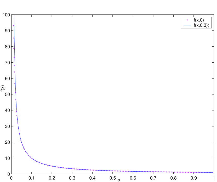
Figure 1. Frequency spectrum $f(x,t)=g(x,t)/(x(1-x))$ at times $t=0$ and $t=0.3$ with parameter values $R=40$ and $S=0$. Obtained by numerically integrating the PDE. The values of $f$ are restricted to the interval $[0,100]$.

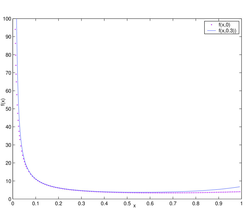
Figure 2. Frequency spectrum $f(x,t)=g(x,t)/(x(1-x))$ at times $t=0$ and $t=0.3$ with parameter values $R=40$ and $S=+2$. Obtained by numerically integrating the PDE. The values of $f$ are restricted to the interval $[0,100]$.

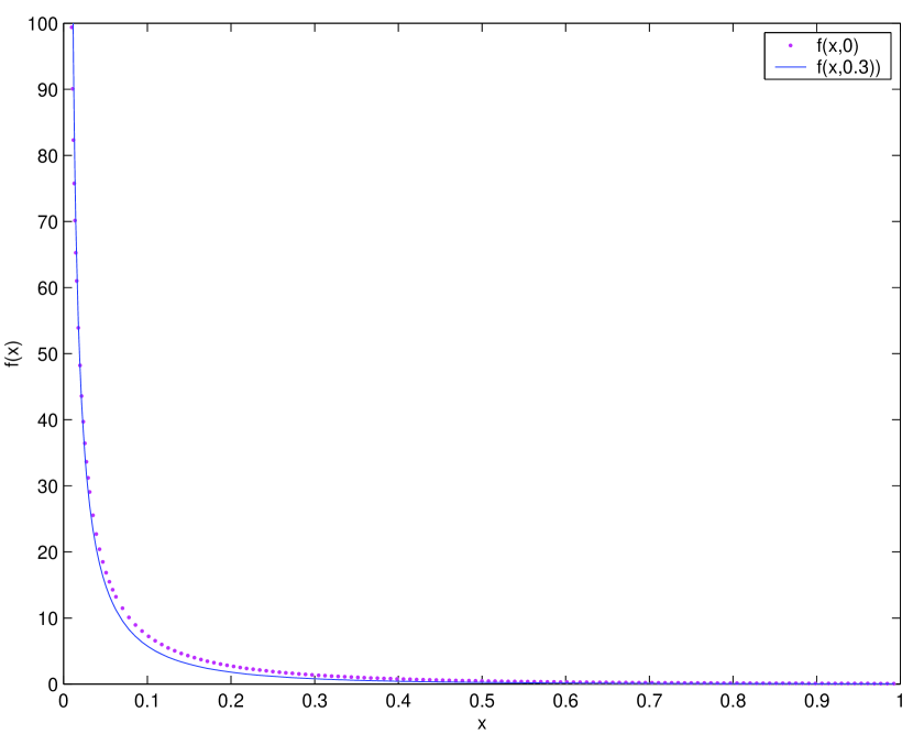
Figure 3. Frequency $f(x,t)=g(x,t)/(x(1-x))$ at times $t=0$ and $t=0.3$ with parameter values $R=40$ and $S=-2$; Obtained by numerically integrating the PDE. The values of $f$ are restricted to the interval $[0,100]$.

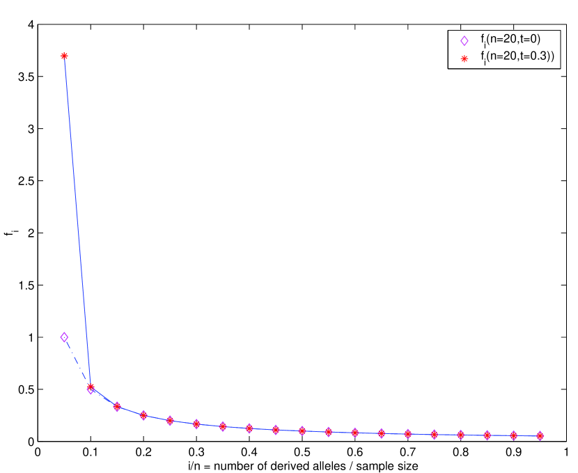
Figure 4. Finite spectrum for a sample size $n=20$ at times $t=0$ and $t=0.3$ with parameter values $R=40$ and $S=0$. Obtained by numerically integrating the system of ODEs for the moments of $g(\cdot,t)$.

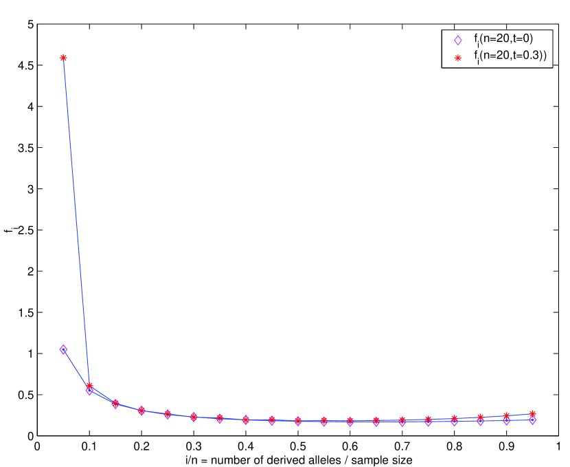
Figure 5. Finite spectrum for a sample size $n=20$ at times $t=0$ and $t=0.3$ with parameter values $R=40$ and $S=+2$. Obtained by numerically integrating the system of ODEs for the moments of $g(\cdot,t)$.

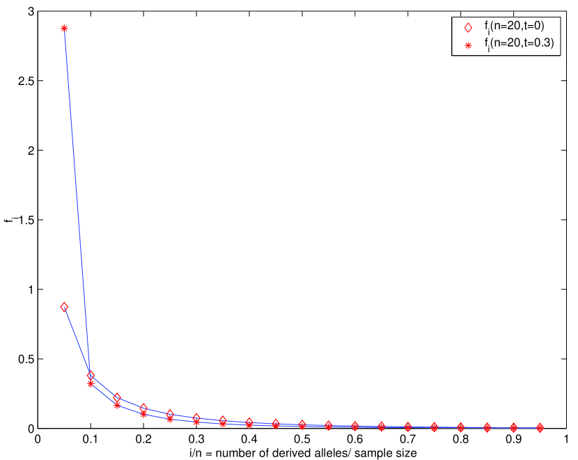
Figure 6. Finite spectrum for a sample size $n=20$ at times $t=0$ and $t=0.3$ with parameter values $R=40$ and $S=-2$. Obtained by numerically integrating the system of ODEs for the moments of $g(\cdot,t)$.

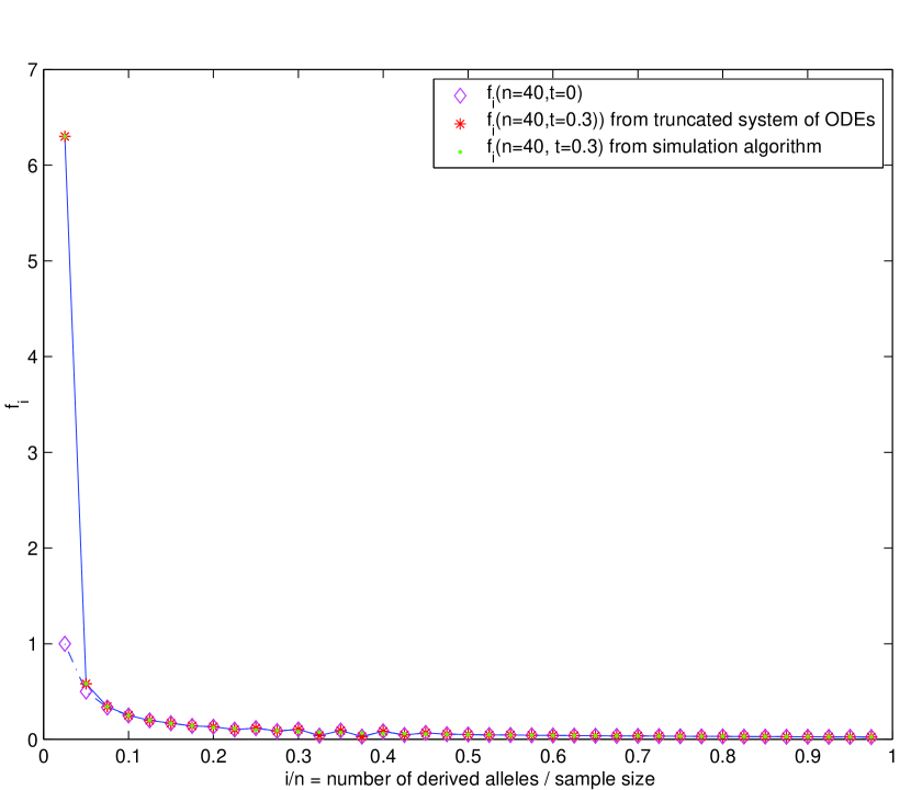
Figure 7. Finite spectrum for a sample size $n=40$ at times $t=0$ and $t=0.3$ with parameter values $R=40$ and $S=0$. Obtained by numerically integrating the system of ODEs for the moments of $g(\cdot,t)$. Compared at time $t=0.3$ with results from the simulation algorithm of Griffiths and Tavaré.

References

- Braverman et al. (1995) Braverman, J., Hudson, R. R., Kaplan, N. L., Langley, C. H., Stephan, W., 1995. The hitchhiking effect on the site frequency spectrum of DNA polymorphisms. Genetics 140, 783–796.
- Bustamante et al. (2005) Bustamante, C. D., Fledel-Alon, A., Williamson, S., Nielsen, R., Todd Hubisz, M., Glanowski, S., Tanenbaum, D. M., White, T. J., Sninsky, J. J., Hernandez, R. D., Civello, D., Adams, M. D., Cargill, M., Clark, A. G., 2005. Natural selection on protein-coding genes in the human genome. Nature 437 (7062), 1153–1157.
- Bustamante et al. (2001) Bustamante, C. D., Wakeley, J., Sawyer, S., Hartl, D. L., 2001. Directional selection and the site-frequency spectrum. Genetics 159 (4), 1779–1788.
- Ewens (2004) Ewens, W. J., 2004. Mathematical Population Genetics: I. Theoretical Introduction, 2nd Edition. Interdisciplinary Applied Mathematics. Springer.
- Fay et al. (2002) Fay, J. C., Wyckoff, G. J., Wu, C.-I., 2002. Testing the neutral theory of molecular evolution with genomic data from Drosophila. Nature 415 (6875), 1024–1026.
- Fisher (1930) Fisher, R. A., 1930. The distribution of gene ratios for rare mutations. Proceedings of the Royal Society of Edinburgh 50, 205–220.
- Gradshteyn and Ryzhik (2000) Gradshteyn, I. S., Ryzhik, I. M., 2000. Table of integrals, series, and products, sixth Edition. Academic Press Inc., San Diego, CA, translated from the Russian, Translation edited and with a preface by Alan Jeffrey and Daniel Zwillinger.
- Griffiths (2003) Griffiths, R. C., 2003. The frequency spectrum of a mutation, and its age, in a general diffusion model. Theoretical Population Biology 64 (2), 241–251.
- Griffiths and Tavaré (1998) Griffiths, R. C., Tavaré, S., 1998. The age of a mutation in a general coalescent tree. Stochastic Models 14, 273–295.
- Hill (1972) Hill, W. G., 1972. Effective size of populations with overlapping generations. Theoretical Population Biology 3, 278–289.
- Kim and Stephan (2002) Kim, Y., Stephan, W., 2002. Detecting a local signature of genetic hitchhiking along a recombining chromosome. Genetics 160 (2), 765–777.
- Kimura (1955) Kimura, M., 1955. Solution of a process of random genetic drift with a continuous model. Proceedings of the National Academy of Sciences USA. 41, 144–150.
- Kimura (1964) Kimura, M., 1964. Diffusion models in population genetics. Journal of Applied Probability 1, 177–232.
- Kimura (1969) Kimura, M., 1969. The number of heterozygous nucleotide sites maintained in a finite population due to steady flux of mutations. Genetics 61, 893–903.
- Knight (1981) Knight, F. B., 1981. Essentials of Brownian motion and diffusion. Vol. 18 of Mathematical Surveys. American Mathematical Society, Providence, R.I.
- Nei et al. (1975) Nei, M., Maruyama, T., Chakraborty, R., 1975. The bottleneck effect and genetic variability in populations. Evolution 29, 1–10.
- Nielsen (2000) Nielsen, R., 2000. Estimation of population parameters and recombination rates from single nucleotide polymorphisms. Genetics. 154 (2), 931–942.
- Pitman and Yor (1982) Pitman, J., Yor, M., 1982. A decomposition of Bessel bridges. Z. Wahrsch. Verw. Gebiete 59 (4), 425–457.
- Polanski and Kimmel (2003) Polanski, A., Kimmel, M., Sep 2003. New explicit expressions for relative frequencies of single-nucleotide polymorphisms with application to statistical inference on population growth. Genetics 165 (1), 427–436.
- Reich and Lander (2001) Reich, D. E., Lander, E. S., 2001. On the allelic spectrum of human disease. Trends in Genetics 17 (9), 502–510.
- Rogers and Williams (2000) Rogers, L. C. G., Williams, D., 2000. Diffusions, Markov processes, and martingales. Vol. 2. Cambridge Mathematical Library. Cambridge University Press, Cambridge, reprint of the second (1994) edition.
- Sawyer and Hartl (1992) Sawyer, S. A., Hartl, D. L., 1992. Population genetics of polymorphism and divergence. Genetics 132 (4), 1161–1176.
- Tajima (1989) Tajima, F., 1989. The effect of change in population size on DNA polymorphism. Genetics 123 (3), 597–602.
- Wakeley et al. (2001) Wakeley, J., Nielsen, R., Liu-Cordero, S. N., Ardlie, K., 2001. The discovery of single-nucleotide polymorphisms: And inferences about human demographic history. American Journal of Human Genetics 69 (6), 1332–1347.
- Williams (1974) Williams, D., 1974. Path decomposition and continuity of local time for one-dimensional diffusions. I. Proc. London Math. Soc. (3) 28, 738–768.
- Williamson et al. (2004) Williamson, S., Fledel-Alon, A., Bustamante, C. D., 2004. Population genetics of polymorphism and divergence for diploid selection models with arbitrary dominance. Genetics 168 (1), 463–475.
- Williamson et al. (2005) Williamson, S. H., Hernandez, R., Fledel-Alon, A., Zhu, L., Nielsen, R., Bustamante, C. D., May 19, 2005. Simultaneous inference of selection and population growth from patterns of variation in the human genome. Proceedings of the National Academy of Sciences USA. 102, 7882–7887.
- Wooding and Rogers (2002) Wooding, S., Rogers, A., 2002. The matrix coalescent and an application to human single-nucleotide polymorphisms. Genetics 161 (4), 1641–50.
- Wright (1931) Wright, S., 1931. Evolution in Mendelian populations. Genetics 16, 97–159.
- Wright (1938) Wright, S., 1938. The distribution of gene frequencies under irreversible mutation. Proceedings of the National Academy of Sciences of the United States of America 24, 253–259.