Temporal and dimensional effects in evolutionary graph theory

Abstract

The spread in time of a mutation through a population is studied analytically and computationally in fully-connected networks and on spatial lattices. The time, $t_{*}$, for a favourable mutation to dominate scales with population size $N$ as $N^{(D+1)/D}$ in $D$-dimensional hypercubic lattices and as $N\ln N$ in fully-connected graphs. It is shown that the surface of the interface between mutants and non-mutants is crucial in predicting the dynamics of the system. Network topology has a significant effect on the equilibrium fitness of a simple population model incorporating multiple mutations and sexual reproduction. Includes supplementary information.

Population models have been used to study various problems in evolutionary biology Baake and Gabriel (2000); Hartl (2000); Ewens (1979). Generally, these models assume a non-spatial population Kimura (1964); Kimura and Maruyama (1966); Kondrashov (1988); Cohen et al. (2005). As competition in the wild is generally local and spatial Tilman and Kareiva (1997), the impact of this assumption needs to be examined carefully. There is evidence that spatially subdividing populations can change the dynamics of alleles spreading through a population Whitlock (2003); Maruyama (1970); Slatkin (1981). Spatial structure has also been shown to change the dynamics of co-operative gamesNowak (1993); Hauert and Doebeli (2004).

Recently, Lieberman et al.Lieberman et al. (2005) introduced ’evolutionary graph theory’ to allow the effects of spatial structure on evolutionary dynamics to be studied directly, placing Moran’s processMoran (1958) on a network. On a $2D$-network, this model is equivalent to the Williams-Bjerknes model Williams and Bjerknes (1972). Lieberman et al. showed that, in networks characterized by a symmetric stochastic matrix, mutants have a fixation probability that depends on the mutant fitness, $r$ (defined relative to a background wild-type fitness of unity), and on the number of nodes in the system, $N$, but which is the same for all members of that class of networks. Other networks, such as scale-free networks, were found to lead to different fixation probabilities Lieberman et al. (2005).

The main aim of this paper is to investigate analytically and numerically the dynamics of evolution in networks with symmetric stochastic matrices. We demonstrate that the mutant fixation time significantly depends on the network topology and dimensionality (as well as $N$ and $r$), despite the fact that the fixation probability in all these networks is the same in the limit of infinite time. In a related model, allowing for simultaneous multiple mutations, the equilibrium fitness is defined by a balance equation with a typical time much less than the fixation time and hence the equilibrium fitness of a population model depends on the Euclidean dimensionality of the network. Thus, approximating realistic spatial networks by fully-connected graphs results in an appreciable overestimate of the equilibrium fitness. We also demonstrate that the topology of the network affects differently the equilibrium fitness of sexual and asexual populations.

In ’evolutionary graph theory’ Lieberman et al. (2005), each vertex of a graph represents an individual with fitness $r$ for a mutant and $1$ for a wild-type organism. On each turn (time step), an individual on a node $i$ is selected for reproduction, with a probability linearly proportional to its fitness. A clone of the selected individual is placed onto one of the nodes, $j$, connected to it by the network which is chosen with a probability, $w_{ij}$, given by the stochastic matrix. The individual previously at $j$ is replaced, conserving the population size. Fixation of the mutant gene occurs when the number of mutants, $m$, reaches $N$, and extinction occurs when $m=0$.

Here, we consider the special class of graphs with fixed node connectivity, $Z$, and $w_{ij}=w_{ji}=1/Z$ for connected nodes and $w_{ij}=0$ otherwise, and analyse the spread of an advantageous mutation ($r>1$).

The number of mutants, $m(t)$, increases, decreases or remains unchanged in each time step with probabilities, $p_{\uparrow}$, $p_{\downarrow}$, and $1-p_{\uparrow}-p_{\downarrow}$, respectively. Changes occur at the interface consisting of $A$ links between mutants and wild-types. The value of $p_{\uparrow}$ is given by the probability that a given mutant reproduces in the turn, $p_{m,\text{repr}}=r/[mr+(N-m)\times 1]$, multiplied by the number of mutants and $p_{m,\text{inter}}=A/(mZ)$, which is the probability that the mutant passes its offspring across the interface, i.e. $p_{\uparrow}=(A/Z)r/[mr+(N-m)]$. Similarly, $p_{\downarrow}=(A/Z)\times 1/(mr+(N-m))$. Taking the deterministic (fluctuations are ignored), continuous-time and continuous-mutant population number approximation ($1\ll m\ll N$), we obtain the following equation Paley et al. (2006a)

$$\frac{\text{d}m}{\text{d}t}\simeq R_{\uparrow}-R_{\downarrow}=\frac{A}{Z}\frac{r-1}{mr+(N-m)}~{},$$ (1)

where $R_{\uparrow(\downarrow)}=p_{\uparrow(\downarrow)}/\Delta t$ (with $\Delta t=1$ being the simulation time step length), i.e. the change in the mutant population per time step is, on average, equal to the probability that the population grows minus the probability that it decreases.

The number of links between mutants and non-mutants may vary with $m(t)$, and for some networks, the functional form of $A(m)$ is known exactly. For example, in the linear chain ($Z=2$, periodic boundaries), $A=2$ for $m<N$ and $A=0$ for $m=N$, and hence the solution of Eq. (12), with $m(0)=1$, is straightforward,

$$m(t)=-\frac{N}{r-1}+\sqrt{\left(\frac{N}{r-1}+1\right)^{2}+2t}~{},$$ (2)

for $t\leq t_{\text{f}}=N^{2}(r+1)/(r-1)$, where the upper limit $t_{\text{f}}$ is the fixation time which scales quadratically with $N$.

In the case of a fully-connected graph ($Z=N-1$), $A=m(N-m)$, and the rate equation can be solved implicitly, resulting in (for $m(0)=1$):

$$t=\frac{(N-1)}{(r-1)}\ln\left[\frac{(N-1)^{r}m}{(N-m)^{r}}\right]~{}.$$ (3)

Simulations support these analytical expressions (see Fig. 1(a) and (d)). The continuum approximation used in Eq. (12) breaks down for $m\to 0$ or $m\to N$. This causes large fluctuations at the initial stage of invasion, which lead to displacements of $m(t)$ along the time axis (see Fig. 1), being equivalent to variations in the initial condition. The shape of the curve does not change and agrees well with the analytical predictions. It might be biologically important that the size of the initial fluctuations increases with decreasing mutant fitness Rozen et al. (2002), as can be clearly seen from Fig. 1(d). The fluctuations, which separate the curves of each simulation run are of greater consequence in the high-dimension systems where the overall time-scales are shorter.

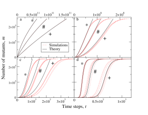
Figure 1: (Color online) Number of mutants, $m$, vs. time, $t$, in the models defined on networks of different topologies: (a) linear chain, (b) square lattice, (c) cubic lattice and (d) fully-connected graph. Predictions (solid black line) are compared to data from six simulation runs (dashed red line). The plots marked ’$*$’ are for mutants of $r=3$, ’$\#$’ corresponds to $r=2$, and ’$+$’ to $r=1.5$. $N=250,000$ has been used in simulations for all networks except (c) with $N=250,047$. The theoretical plot in (a) overlays the simulation data.

For square ($Z=4$) and cubic ($Z=6$) lattices, the relationship between $A$ and $m$ is multi-valued and unknown. The current belief is that the mutant/non-mutant interface is a self-affine surface with

$$A=\beta m^{\gamma}~{},$$ (4)

and $\gamma=(D-1)/D$ Meakin (1993), which is consistent with our numerical data (see Table 1).

Table 1: Values for $\gamma$ found from fits to Eq. (13) with 16 realisations used for each fit. In the 2D case, fits were performed with between 60,000 and 150,000 mutants; in the 3D case, between 45,000 and 75,000 mutants were used.

Mutant fitness, $r$	Square lattice, $\gamma$	Cubic lattice, $\gamma$
1.5	$0.513\pm 0.014$	$0.684\pm 0.012$
2	$0.504\pm 0.008$	$0.700\pm 0.012$
3	$0.512\pm 0.008$	$0.692\pm 0.012$
100	$0.509\pm 0.006$	$0.698\pm 0.007$

Using the numerical estimates for $\beta$ and $\gamma=(D-1)/D$, the rate Eq. (12) can be solved implicitly for $2D$- and $3D$-lattices ($m(0)=1$),

$$t=\frac{Z}{\beta}\left(\frac{1}{2-\gamma}\left(m^{2-\gamma}-1\right)+\frac{N}{(1-\gamma)(r-1)}\left(m^{1-\gamma}-1\right)\right)~{}.$$ (5)

Numerical simulations are in better agreement with analytical predictions in the case of $2D$- than $3D$-lattices. Both predictions fail when edge effects (above the inflexion points in Figs. 1 (b, c) for simulations) become important, i.e. at sufficiently large times. The systematic deviation, overestimating the mutant spread speed, of the simulated data from analytical predictions is due to the violation of Eq. (13) (see Table 1) for small times, when the number of mutants is small and one is far from the asymptotic regime. This effect is more significant in the cubic lattice, which tallies with work on Eden growth exhibiting more pronounced crossover effects in higher dimensions Devillard and Stanley (1989). These deviations are also more substantial when mutants have a smaller comparative fitness (cf. curves for different values of $r$ in Fig. 1 (b, c)). Real favourable mutations generally confer an advantage far smaller than 50% (corresponding to $r=1.5$ in Fig. 1) Rozen et al. (2002), and thus this discrepancy, and early fluctuations, are potentially of importance in biological systems. The less-biased errors from the approximations in Eq. (12) are present in all the simulations, and, for a given $r$, are of similar magnitude in time - the spread of data in time is of a similar magnitude in the body of the plot for all the system types, but shows up most in fully-connected systems which exhibit the shortest time to fixation.

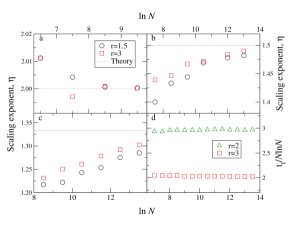
Figure 2: (Color online) Relationship between scaling exponents for fixation time and population size: (a) Linear chain; (b) Square lattice; (c) Cubic lattice; (d) Fully-connected graph. For (a)-(c), theory predicts $t_{f}\propto N^{\eta}$. Using simulations for system sizes spaced at $\ln N=0.5$ intervals, least-square fits were performed over three adjacent times to obtain $\eta$. Each point is therefore an approximation to the gradient of a $\ln t_{f}$ vs $\ln N$ plot at the point. The predicted scaling ($\eta=D/(D+1)$) is shown with dashed lines. For (d), the theory predicts that the time to fixation on a fully-connected graph divided by $N\ln N$ will be constant. Between 100 and 3300 data points were averaged for each value of $t_{f}$.

It follows from Eqs.(2)-(5) that the typical time, $t_{*}$, taken for a mutant to dominate the graph (i.e. to occupy a large fraction of sites, $m(t_{*})\sim N$) depends strongly on the network topology. In a fully-connected graph, $t_{*}$ scales as $N\ln N$, and, in a $D$-dimensional Euclidian network, as $N^{(D+1)/D}$. Fig. 2 shows the approach to this predicted scaling. The exponents for linear chains (a) and fully-connected graphs (d) approach the predictions at very small sizes compared to $2D$- and $3D$-lattices, which is due to the finite-size effects inherent in using Eq. 13.

The above analysis was for a very simple model, with only one mutation present at any time. However, in realistic biological systems, multiple mutations can occur and interact. To investigate these effects, we have modified the model by allowing offspring not to be perfect clones of their parents. In such a model, the network topology has a significant impact on the evolved, equilibrium fitness of the population. We also look at the effects of sexual reproduction, with Mendelian recombination rules, and demonstrate that network topology also affects sexual populations, but in a different way to asexual ones.

In the asexual model with multiple mutations, each time that an offspring is produced, it is subject to a possible mutation. Mutations occur with a probability, $\mu$, and increase the fitness with probability $p$, or decrease it with probability $1-p$. The fitness increment/decrement is the same, $\Delta_{0}$, i.e. offspring are produced from clones of their parents, but with a stochastic change in their fitness $r_{\text{offspring}}=r_{\text{parent}}+\Delta$. The value of $\Delta$ is drawn from a probability distribution function, $\rho(\Delta)$, of the form,

$$\rho(\Delta)=(1-\mu)\delta(\Delta)+\mu[(1-p)\delta(\Delta+\Delta_{0})+p\delta(\Delta-\Delta_{0})]~{},$$ (6)

(with $\Delta_{0}>0$). In this model (as we have observed numerically), the population reaches an equilibrium fitness, caused by mutation-selection balance Bürger (2000), proportional to $\Delta_{0}$ provided that the initial dynamics do not lead to extinction (in which all individuals’ fitnesses reach zero) and that $p<0.5$ (with more positive mutations than negative mutations, the fitness tends to infinity). In the fully-connected system, this is the model studied in Ref. Ridgway et al. (1998). Fig. 3 shows that the equilibrium fitness of asexual populations significantly depends on the dimensionality of the network as well as on the population size Lande (1995), with higher dimensional systems exhibiting greater equilibrium fitnesses. The networks found (Fig. 1) to have a slower spread of mutants lead to a lower fitness in the model with multiple mutations. The slower spread means that individuals compete with closely related neighbours and when a fit individual reproduces, it is more likely to replace another fit individual. It can be seen from Fig. 3 that the fitness increase with $N$ saturates for the spatial systems. For fully-connected systems of up to 250,000 nodes, no saturation was observed (cf. Ref. Ridgway et al. (1998)).

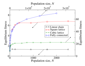
Figure 3: (Color online) Relationship of equilibrium fitness to population size, $N$, and network topology in an asexual population for $\mu=0.4$, $\Delta_{0}=1$ and $p=0.1$ (cf. Eq. (17)). Data were averaged over 50 realizations and errors are smaller than the symbols. Lines are guides to the eye only. The linear-chain and square-lattice systems use the left and bottom axes; the cubic-lattice and fully-connected systems use the top and right axes. Initial condition: all fitnesses set to unity. The numbers measuring equilibrium fitness are not direct measures of biological reproduction rates, being scaled by $\Delta_{0}$.

To study a sexual population, it is necessary to introduce multiple genes per individual, allowing recombination. We study an additive model (see e.g. Maynard Smith (1968)) in which each individual has $G$ genes. Each gene is characterised by a number (quality factor), and the fitness of the individual is the sum of these quality factors. When an individual is chosen for reproduction, a partner is selected at random from the nodes connected to it and the offspring is produced by a Mendelian shuffling of the genes. The above criteria define hermaphrodite haploids (bisexual individuals with a single copy of each gene). Mutations are applied as in the asexual system, but now each gene is subject to a possible mutation. In Fig. 4, the equilibrium fitness of the sexual population versus $N$ is shown for different network topologies, demonstrating that the dimensionality of the network also affects the fitness of sexual populations, with higher dimensionality networks again leading to increased fitnesses. However, the effect is not as large as for the asexual populations. A saturation equilibrium fitness with $N$ was not observed in the $2D$-, $3D$-lattices or fully-connected systems for $N\leq 250,000$ nodes. The sexual populations were found to have higher equilibrium fitnesses than the asexual fitnesses for the parameter range $G\gtrsim 10,\mu\gtrsim 0.01,p\lesssim 0.1,N\gtrsim 200$. The general principle that the advantage of sex is greater (and the fitness is lower) in lattices than in fully-connected graphs holds over a range of variables.

It should be noted that in an asexual system created by suppressing the recombination in a sexual system (i.e. an asexual population with genes) the fitness depends only on the product $\mu G$. The populations in Figs 3-4 are therefore directly comparable, and the differences are due to the presence or absence of recombination. The ’slower’ networks still see the fitness disadvantage, as with the asexual system. However, the correlations in the population fitness (a fit neighbour being surrounded by other fit individuals) now give a benefit as well as a disadvantage - a fit individual is more likely to mate with a fit individual as well as to replace one with her offspring. The sexual process may also reduce the degree of spatial frustration, as genes can pass to second-nearest neighbours, potentially speeding up the spread of mutations. A larger advantage for sex does not necessarily mean, however, that the establishment/maintenance of sex would occur more readily Paley et al. (2007) in a spatial network than in the fully connected systems usually studied (to be discussed elsewhere).

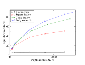
Figure 4: (Color online) Relationship of equilibrium fitness to population size, $N$, and network topology in a sexual population for $\mu=0.04$, $\Delta_{0}=1$ and $p=0.1$ (c.f. Eq. (17)) and $G=10$ (so that $\mu G=0.4$ has the same value as $\mu$ in Fig. 3). The data were averaged over 50 realizations and the errors are smaller than the symbols used. Lines are guides to the eye only. Initial condition: all gene quality factors set to unity.

To conclude, we have demonstrated that the spatial nature of populations (dimensionality of the population network) is of significant importance for the dynamics of evolution. The following effects have been found for populations defined on networks of higher dimensionality (e.g. fully-connected graph as compared to a square lattice): (i) faster spread of a mutation, (ii) greater values of equilibrium fitness in both sexual and asexual populations, in a model in which mutations do not have time to fixate before the next mutation is introduced into the system. Whilst both sexual and asexual populations have increased fitnesses for higher dimensional networks, the effect of topology on each is markedly different.

CJP thanks the EPSRC for financial support.

I Supplementary information

II The discrete origins of the master equation

Each individual on the graph has a fitness, 1 (wild-type) or $r$ (mutant) in this part of the paper, associated with it. On each turn, an individual is selected for reproduction, with a probability proportional to its fitness. A clone of the selected individual is placed onto one of the nodes connected to it by the network. The individual that previously occupied the node is replaced, conserving the population size, $N$.

For the spread of mutants, the important events are those that occur at the interface between mutants and non-mutants. At a given connection between a mutant and a non-mutant node, the probability that an event occurs at one of the nodes in a turn is:

$$p_{conn}=\frac{1+r}{mr+(N-m)}~{}.$$ (7)

At a given interface link there must be a wild type (fitness of unity) and mutant individual (r). The probability of selecting one of these is normalised by the total mutant ($m\times r$) and wild type ($[N-m]\times 1$) fitness. Given that an event has happened at a node linked to a particular connection between mutant and non-mutant, the probability that the offspring is placed across this connection is $1/Z$ where $Z$ is the connectivity of each node. In total, there are $A$ links between mutants and non-mutants. The probability that, in a given turn, an event happens across the boundary is:

$$p_{boundary}=\frac{A}{Z}\frac{1+r}{mr+(N-m)}~{}.$$ (8)

Therefore, the probability that, in a given turn, the population of mutants increases by one is:

$$p_{\uparrow}=\frac{A}{Z}\frac{1+r}{mr+(N-m)}\frac{r}{1+r}~{}.$$ (9)

The probability that the mutant population shrinks by one is

$$p_{\downarrow}=\frac{A}{Z}\frac{1+r}{mr+(N-m)}\frac{1}{1+r}~{}.$$ (10)

This can be written as a discrete master equation, where the probability that there are $m$ mutants in the system at time $t$ is given by:

$$P_{m,t}=p_{\uparrow}P_{m-1,t-1}+p_{\downarrow}P_{m+1,t-1}+(1-p_{\uparrow}-p_{\downarrow})P_{m,t-1}~{}.$$ (11)

Alternatively, the continuum, deterministic approximation can be taken, where the probability of increase minus the probability of decrease per time-step in mutant population leads to an average rate of increase (valid for $1<<m<<N$):

$$\frac{dm}{dt}=R_{\uparrow}-R_{\downarrow}=\frac{A}{Z}\frac{r-1}{mr+(N-m)}~{},$$ (12)

where $R_{\uparrow(\downarrow)}=p_{\uparrow(\downarrow)}/\Delta t$ (with $\Delta t=1$ being the simulation time step length). This is equation (1) in Paley et al. (2006b).

III Derivation of the relation between the number of mutants and time on a lattice

We use the approximation,

$$A=\beta m^{\gamma}~{},$$ (13)

and place this into equation (12) before integrating.

$$\int_{1}^{m}\frac{mr+(N-m)}{m^{\gamma}}\mathrm{d}m=\int_{0}^{t}\frac{\beta}{Z}(r-1)\mathrm{d}t~{}.$$ (14)

This integral can be solved to give:

$$(r-1)\frac{m^{2-\gamma}}{2-\gamma}+N\frac{m^{1-\gamma}}{1-\gamma}-(r-1)\frac{1}{2-\gamma}-N\frac{1}{1-\gamma}=\frac{\beta}{Z}(r-1)t~{},$$ (15)

which can be re-arranged to give equation (5) in Paley et al. (2006b).

IV Explanation of the equation describing the introduction of new mutations

In the second part of the paper, a model is introduced in which parents do not necessarily produce perfect offspring. The offspring’s fitness is related to that of the parent by the following formula:

$$r_{\text{offspring}}=r_{\text{parent}}+\Delta~{}.$$ (16)

The difference in the fitnesses, $\Delta$, is taken from a probability distribution,

$$\rho(\Delta)=(1-\mu)\delta(\Delta)+\mu(1-p)\delta(\Delta+\Delta_{0})+\mu p\delta(\Delta-\Delta_{0})~{}.$$ (17)

This distribution consists of three weighted delta-functions, representing the three discrete possibilities. With probability $\mu(1-p)$ (the probability that a mutation occurs multiplied by the probability that it is deleterious), the offspring will have a fitness of $\Delta_{0}$ less than that of their parent ($\Delta=-\Delta_{0}$). With probability $\mu p$, the offspring will have a fitness of $\Delta_{0}$ more than that of their parent, representing an advantageous mutation. With probability $1-\mu$, no mutation will have occurred and the offspring will have the same fitness as the parent.

References

- Baake and Gabriel (2000) E. Baake and W. Gabriel, Ann. Rev. Com. Phys. 7, 203 (2000).
- Hartl (2000) D. Hartl, A primer of population genetics (Sinauer, 2000).
- Ewens (1979) W. Ewens, Mathematical population genetics (Springer-Verlag, 1979).
- Kimura (1964) M. Kimura, J. Appl. Prob. 1, 177 (1964).
- Kimura and Maruyama (1966) M. Kimura and T. Maruyama, Genetics 54, 1337 (1966).
- Kondrashov (1988) A. Kondrashov, Nature 336, 435 (1988).
- Cohen et al. (2005) E. Cohen, D. Kessler, and H. Levine, Phys. Rev. Lett. 94, 098102 (2005).
- Tilman and Kareiva (1997) D. Tilman and P. Kareiva, eds., Spatial ecology: the role of space in population dynamics and interspecific interactions (Princeton University Press, 1997).
- Whitlock (2003) M. Whitlock, Genetics 164, 767 (2003).
- Maruyama (1970) T. Maruyama, Theor. Pop. Biol. 1, 273 (1970).
- Slatkin (1981) M. Slatkin, Evolution 35, 477 (1981).
- Nowak (1993) M. Nowak, Int. J. Bifurcation Chaos 3, 35 (1993).
- Hauert and Doebeli (2004) C. Hauert and M. Doebeli, Nature 428, 643 (2004).
- Lieberman et al. (2005) E. Lieberman, C. Hauert, and M. Nowak, Nature 433, 312 (2005).
- Moran (1958) P. Moran, Proc. Camb. Phil. Soc. 54, 60 (1958).
- Williams and Bjerknes (1972) T. Williams and R. Bjerknes, Nature 236, 19 (1972).
- Paley et al. (2006a) C. Paley, S. Taraskin, and S. Elliott, q-bio.PE/0609013 (2006a).
- Rozen et al. (2002) D. Rozen, J. de Visser, and P. Gerrish, Current biology 12, 1040 (2002).
- Meakin (1993) P. Meakin, Phys. Rep. 235, 189 (1993).
- Devillard and Stanley (1989) P. Devillard and H. Stanley, Physica A 160, 298 (1989).
- Bürger (2000) R. Bürger, The mathematical theory of selection, recombination, and mutation (Wiley, 2000).
- Ridgway et al. (1998) D. Ridgway, H. Levine, and D. Kessler, J. Stat. Phys. 90, 191 (1998).
- Lande (1995) R. Lande, Conservation Biology 9, 782 (1995).
- Maynard Smith (1968) J. Maynard Smith, Nature 219, 1114 (1968).
- Paley et al. (2007) C. Paley, S. Taraskin, and S. Elliott, Naturwissenschaften pp. DOI 10.1007/s00114–007–0220–8 (2007).
- Paley et al. (2006b) C. Paley, S. Taraskin, and S. Elliott, q-bio.PE/0604009 (2006b).