[

NEW COMPUTATIONAL APPROACHES TO ANALYSIS OF INTERBEAT INTERVALS IN HUMAN SUBJECTS

]

1. Introduction

Complex, self- regulating systems such as the human heart must process inputs with a broad range of characteristics to change physiological data and time series.¹³ Many of these physiological time series seem to be highly chaotic, represent nonstationary data, and fluctuate in an irregular and complex manner. One hypothesis is that the seemingly chaotic structure of physiological time series arises from external and intrinsic perturbations that push the system away from a homeostatic set point. An alternative hypothesis is that the fluctuations are due, at least in part, to the system s underlying dynamics. In this review, we describe new computational approaches based on new theoretical concepts for analyzing physiological time series. We ll show that the application of these methods could potentially lead to a novel diagnostic tool for distinguishing healthy individuals from those with congestive heart failure (CHF).

Physiological Time Series

Recent research suggests that physiological time series can possess fractal and self-similar properties, which are characterized by the existence of long-range correlations (with the correlation function being a power-law type). However, until recently, the analysis of such fluctuations fractal properties was restricted to computing certain characteristics based on the second moment of the data, such as the power spectrum and the two-point autocorrelation function. These analyses indicated that the fractal behavior of healthy, free-running physiological systems could be characterized, at least in some cases, by 1/f-like scaling of the power spectra over a wide range of time scales.^4,5 A time series that exhibits such long-range correlations with a power-law correlation function and is also homogeneous (different parts of the series have identical statistical properties) is called a monofractal series. However, many physiological time series are inhomogeneous in the sense that distinct statistical and scaling properties characterize different parts of the series. In addition, there is some evidence that physiological dynamics can exhibit nonlinear properties.^6-12 Such features are often associated with multifractal behavior the presence of long-range power-law correlations in the higher moments of the time series which, unlike monofractals, are nonlinear functions of the second moment s scaling exponents.¹³ Up until recently, though, robust demonstration of multifractality of nonstationary time series was hampered by problems related to significant bias in the estimates of the data s singularity spectrum, due to the time series diverging negative moments. A new wavelet-based multifractal formalism helps address such problems.¹³ Among physiological time series, the study of the statistical properties of heartbeat interval sequences has attracted much attention.^14-17 The interest is at least partly due to the facts that the heart rate is under direct neuroautonomic control; interbeat interval variability is readily measured by noninvasive means; and analysis of heart-rate dynamics could provide important diagnostic and prognostic information. Thus, extensive analysis of interbeat interval variability represents an important quantity for elucidating possibly nonhomeostatic physiological variability. Figure 1 shows examples of cardiac interbeat time series (the output of a spatially and temporally integrated neuroautonomic control system) for healthy individuals and those with CHF. In the conventional approaches to analyzing such data, we would assume the apparent noise has no meaningful structure, so we wouldn t expect to gain any understanding of the underlying system through the study of such fluctuations. Conventional studies that focus on averaged quantities therefore usually ignore these fluctuations in fact, they re often labeled as noise to distinguish them from the true time series of interest. However, by adapting and extending methods developed in modern statistical physics and nonlinear dynamics, the physiological fluctuations in Figure 1 can be shown to exhibit an unexpected hidden scaling structure.^{5,10,13,18,19} Moreover, the fluctuation dynamics and associated scaling features can change with pathological perturbation. These discoveries have raised the possibility that understanding the origin of such temporal structures and their alterations through disease could elucidate certain basic aspects of heart-rate control mechanisms and increase the potential for clinical monitoring. But despite this considerable progress, several interesting features must still be analyzed and interpreted. The theoretical concepts we discuss here are based on the possible Markov properties of the time series; a cascade of information from large time scales to small ones that are built based on increments in the time series; and the extended self-similar properties of the beat-to-beat fluctuations of healthy subjects as well as those with CHF. The method we describe uses a set of data for a given phenomenon that contains a degree of stochasticity and numerically constructs a relatively simple equation that governs the phenomenon. In addition to being accurate, this method is quite general, can provide a rational explanation for complex features of the phenomenon under study, and requires no scaling feature or assumption. As we analyze cardiac interbeat intervals, we ll also look at new methods for computing the Kramers-Moyal (KM) coefficients for the increments of interbeat intervals fluctuations,$\Delta x(\tau)=[x(t+\tau)-x(t)]/\sigma_{\tau}$, where $\sigma_{\tau}$ is the standard deviations of the increments in the interbeats data. Whereas the first and second KM coefficients (representing the drift and diffusion coefficients in a Fokker-Planck [FP] equation) have well-defined values, the third- and fourth-order KM coeffi- cients might be small. If so, we can numerically construct an FP evolution equation for the probability density function, $P(\Delta x,\tau)$ which, in turn, can be used to gain information on the PDF s evolution as a function of the time scale ${\tau}.^{2023}$

Regeneration of Stochastic Processes

Let s start by examining the computations that lead to the numerical construction of a stochastic equation. This equation describes the phenomenon that generates the data set, which is then utilized to reconstruct the original time series. Two basic steps are involved in the numerical analysis of the data and their reconstruction. Data Examination We must first examine the data to see whether they follow a Markov chain and, if so, we estimate the Markov time scale $t_{M}$. As is well known, a given process with a degree of stochasticity can have a finite or an infinite Markov time scale, which is the minimum time interval over which the data can be considered to be a Markov process.^20,24 To determine the Markov scale $t_{M}$, we note that a complete characterization of the statistical properties of stochastic fluctuations of a quantity $x(t)$ requires the numerical evaluation of the joint PDF $P_{n}(x_{1},t_{1};\cdots;x_{n},t_{n})$ for an arbitrary $n$, the number of the data points in the time series $x(t)$. If the time series $x(t)$ is a Markov process, an important simplification can be made as $P_{n}$, the $n$-point joint PDF, is generated by the product of the conditional probabilities $P(x_{i+1},t_{i+1}|x_{i},t_{i})$, for $i=1,\cdots,n-1$. A necessary condition for $x(t)$ to be a Markov process is that the Chapman-Kolmogorov (CK) equation,

$$P(x_{2},t_{2}|x_{1},t_{1})=\int\hbox{d}(x_{3})\;P(x_{2},t_{2}|x_{3},t_{3})\;P(x_{3},t_{3}|x_{1},t_{1})\;,$$ (1)

should hold for any value of $t_{3}$ in the interval $t_{2}<t_{3}<t_{1}$. One should check the validity of the CK equation for various $x_{1}$ by comparing the directly-computed conditional probability distributions $P(x_{2},t_{2}|x_{1},t_{1})$ with the ones computed according to right side of Eq. (1). The simplest way to determine $t_{M}$ for stationary or homogeneous data is the numerical computation of the quantity, $S=|P(x_{2},t_{2}|x_{1},t_{1})-\int\hbox{d}x_{3}P(x_{2},t_{2}|x_{3},t_{3})\,P(x_{3},t_{3}|x_{1},t_{1})|$, for given $x_{1}$ and $x_{2}$, in terms of, for example, $t_{3}-t_{1}$ (taking into account the possible numerical errors in estimating $S$). Then, $t_{M}=t_{3}-t_{1}$ for that value of $t_{3}-t_{1}$ for which $S$ vanishes or is nearly zero (achieves a minimum).

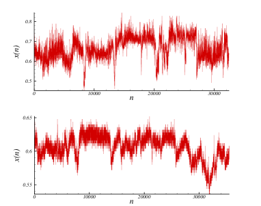
FIG. 1.: Interbeats fluctuations of healthy subjects (top), and those with congestive heart failure (bottom).

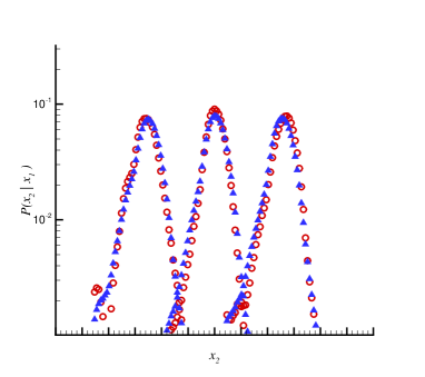
FIG. 2.: Test of Chapman-Kolmogorov equation for $x_{1}=-5$, $x_{1}=0$ and $x_{1}=5$. The bold and open symbols represent, respectively, the directly-evaluated PDF and the integrated PDF. The PDFs are shifted in the vertical directions for better presentation. Values of $x$ are measured in units of the standard deviation.

(2) Numerical construction of an effective stochastic equation that describes the fluctuations of the quantity $x(t)$, representing the time series, constitutes the second step. The CK equation yields an evolution equation for the PDF $P(x,t)$ across the scales $t$. The CK equation, when formulated in differential form, yields a master equation which takes the form of a FP equation:

$$\frac{d}{dt}P(x,t)=\left[-\frac{\partial}{\partial x}D^{(1)}(x,t)+\frac{\partial^{2}}{\partial x^{2}}D^{(2)}(x,t)\right]P(x,t)\;.$$ (2)

The drift and diffusion coefficients, $D^{(1)}(x,t)$ and $D^{(2)}(x,t)$, are computed directly from the data and the moments $M^{(k)}$ of the conditional probability distributions:

$$D^{(k)}(x,t)=\frac{1}{k!}\lim_{\Delta t\to 0}M^{(k)}\;,$$ (3)

$$M^{(k)}=\frac{1}{\Delta t}\int dx^{\prime}(x^{\prime}-x)^{k}P(x^{\prime},t+\Delta t|x,t)\;.$$ (4)

Note that the above FP formulation is equivalent to the following Langevin equation:

$$\frac{d}{dt}x(t)=D^{(1)}(x)+\sqrt{D^{(2)}(x)}\;\;f(t)\;,$$ (5)

where $f(t)$ is a random force with zero mean and Gaussian statistics, $\delta$-correlated in $t$, i.e., $\langle f(t)f(t^{\prime})\rangle=2\delta(t-t^{\prime})$. We note that the numerical reconstruction of a stochastic process does not imply that the data do not contain any correlations, or that the above formulation ignores the correlations.

Equation (5) enables us to reconstruct a stochastic time series $x(t)$, which is similar to the original one in the statistical sense. The stochastic process $x(t)$ is regenerated by iterating Eq. (5) which yields a series of data without memory. To compare the regenerated series with the original $x(t)$, we must take the temporal interval in the numerical discretization of Eq. (5) to be unity (or renormalize it to unity, if need be). However, the Markov time is typically greater than unity. Therefore, we correlate the data over the Markov time scale $t_{M}$, for which there are a number of methods.^21,22,25 A new technique that we have used in our own studies, which we refer to as the kernel method, is one according to which one considers a kernel function $K(u)$ that satisfies the condition that,

$$\int_{-\infty}^{\infty}K(u)du=1\;,$$ (6)

such that the data are determined, or reconstructed, by

$$x(t)=\frac{1}{nh}\sum_{i=1}^{n}x(t_{i})K\left(\frac{t-t_{i}}{h}\right)\;,$$ (7)

where $h$ is the window width. For example, one of the most accurate kernels is the standard normal density function, $K(u)=(2\pi)^{-1/2}\exp(-\frac{1}{2}u^{2})$. In essence, the kernel method represents the the time series as a sum of “bumps” placed at the “observation” points, with its kernel determining the shape of the bumps, and its window width $h$ fixing their width. It is evident that, over the scale $h$, the kernel method correlates the data.

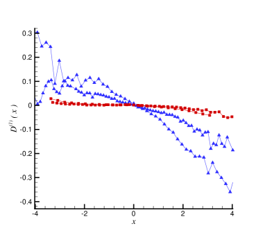
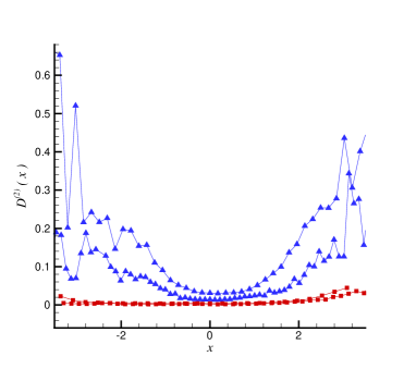
FIG. 3.: The drift and diffusion coefficients $D^{(1)}(x)$ and $D^{(2)}(x)$, estimated by Eq. (3). For the healthy subjects (triangles) $D^{(1)}(x)$ and $D^{(2)}(x)$ follow linear and quadratic behavior in $x$, while for patients with CHF (squares) they follow third- and fourth-order behavior in $x$.

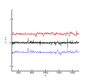
FIG. 4.: The curves show, from top to bottom, the actual interbeat data (for a healthy subject), the regenerated data using the corresponding Langevin equation, and the regenerated data using the kernel method. The time series are shifted in the vertical directions for better presentation.

3. Analysis of Fluctuations in Human Heartbeats

To show how the above reconstruction method is used in practice, and to demonstrate its utility, the method has been applied to reconstruction of the fluctuations in human heartbeats of both healthy and ill subjects by taking $h\simeq t_{M}$. Recent studies^5,19,26,27 reveal that under normal conditions, beat-to-beat fluctuations in the heart rates might display extended correlations of the type typically exhibited by dynamical systems far from equilibrium. It has been argued,²⁶ for example, that the various stages of sleep might be characterized by extended correlations of heart rates separated by a large number of beats. While the existence of extended correlations in the fluctuations of human heartbeats is an interesting and important result, we argue that the Markov time scale $t_{M}$ and the associated drift and diffusion coefficients of the interbeat fluctuations of healthy subjects and those with CHF help one to better distinguish the two classes of subjects, particularly at the early stages of the disease, as these quantities have completely different behaviour for the two classes of subjects.

Both daytime (12:00 pm to 18:00 pm) and nighttime (12:00 am to 6:00 am) heartbeat time series of healthy subjects, and the daytime records of patients with CHF have been analyzed by this method.^45,46 The data base includes 10 healthy subjects (7 females and 3 males with ages between 20 and 50, and average age of 34.3 years), and 12 subjects with CHF (3 females and 9 males with ages between 22 and 71, and average age of 60.8 years). Figure 1 presents the typical data.

As the first step, the Markov time scale $t_{M}$ of the data is computed. From the daytime data for healthy subjects the values of $t_{M}$ are computed to be (all the values are measured in units of the average time scale for the beat-to-beat times of each subject), $t_{M}=3,3,3,1,2,3,3,2,3$ and 2. The corresponding values for the nighttime records are, $t_{M}$ are $3,3,1,3,3,2,3,3,2$ and $3$, respectively, comparable to those for the daytime. On the other hand, for the daytime records of the patients with CHF, the computed Markov time scales are, $t_{M}=151,258,760,542,231,257,864,8,366,393,385$, and 276. Therefore, the healthy subjects are characterized by $t_{M}$ values that are much smaller than those of the patients with CHF. Thus, one has an unambiguous quantity for distinguishing the two classes of patients.

Next, the validity of the CK equation for describing the phenomenon is checked for several $x_{1}$-triplets by comparing the directly-computed conditional probability distributions $P(x_{2},t_{2}|x_{1},t_{1})$ with the ones computed according to right side of Eq. (1). Here, $x$ is the interbeat and for all the samples we define, $x\equiv(x-\bar{x})/\sigma$, where $\bar{x}$ and $\sigma$ are the mean and standard deviations of the interbeat data. In Figure 2, the two PDFs, computed by the two methods, are compared. Assuming the statistical errors to be the square root of the number of events in each bin, the two PDFs are statistically identical.

The corresponding drift and diffusion coefficients, $D^{(1)}(x)$ and $D^{(2)}(x)$, are displayed in Figure 3, demonstrating that, in addition to the Markov time scale $t_{M}$, the two coefficients provide another important indicator for distinguishing the ill from healthy subjects: For the healthy subjects the drift $D^{(1)}$ and the diffusion coefficients $D^{(2)}(x)$ follow (approximately) linear and quadratic functions of $x$, respectively, whereas the corresponding coefficients for patients with CHF follow (approximately) third- and fourth-order equations in $x$. Thus, for the healthy subjects,

$$D^{(1)}(x)=-0.12x\;,$$ (8)

$$D^{(2)}(x)=(5-4.2x+7x^{2})\times 10^{-2}\;,$$ (9)

whereas for the patients with CHF,

$$D^{(1)}(x)=-(26x+18x^{2}+7x^{3})\times 10^{-4}\;,$$ (10)

$$D^{(2)}(x)=(6-7x+5x^{2}+3x^{3}+2x^{4})\times 10^{-4}\;,$$ (11)

which were also obtained by Kuusela.²⁹ For other data bases measured for other patients, the functional dependence of $D^{(1)}$ and $D^{(2)}(x)$ would be the same, but with different numerical coefficients. The order of magnitude of the coefficients would be the same for all the healthy subjects, and likewise for those with CHF (see also Wolf et al.²⁰). Moreover, if one analyzes different parts of the time series separately, one finds, (1) practically the same Markov time scale for different parts of the time series, but with some differences in the numerical values of the drift and diffusion coefficients, and (2) that the drift and diffusion coefficients for different parts of the time series have the same functional forms, but with different coefficients in equations such as (8)-(11). Hence, one can distinguish the data for sleeping times from those patients when they are awake.

There is yet another important difference between the heartbeat dynamics of the two classes of subjects: Compared with the healthy subjects, the drift and diffusion coefficients for the patients with CHF are very small, reflecting, in some sense, their large Markov time scale $t_{M}$. Large Markov times $t_{M}$ imply longer correlation lengths for the data, and it is well-known that the diffusivity in correlated system is smaller than those in random ones. Hence, one may use the Markov time scales, and the dependence of the drift and diffusion coefficients on $x$, as well as their comparative magnitudes, for characterizing the dynamics of human heartbeats and their fluctuations, and to distinguish healthy subjects from those with CHF.

How accurate is the reconstruction method? Shown in Figure 4 is a comparison between the original time series $x(n)$ and those reconstructed by the Langevin equation [by, for example, using Eqs. (5), (8) and (9)] and the kernel method. While both methods generate series that look similar to the original data, the kernel method appears to better mimic the behavior of the original data. To demonstrate the accuracy of Eq. (7), Figure 5 compares the second moment of the stochastic function, $C_{2}(m)=\langle[x(0)-x(m)]^{2}\rangle$, for both the measured and reconstructed data using the kernel method. The agreement between the two is excellent. However, it is well-known that such agreement is not sufficient for proving the accuracy of a reconstruction method. Hence, the accuracy of the reconstructed higher-order structure function, $S_{n}=\langle|x(t_{1})-x(t_{2})|^{n}\rangle,^{28,29}$ was also checked. It was found that the agreement between $S_{n}$ for the original and reconstructed time series for $n\leq 5$ is excellent, while the difference between higher-order moments of the two times series, which are related to the tails of the PDF of the $x-$increments, increases.

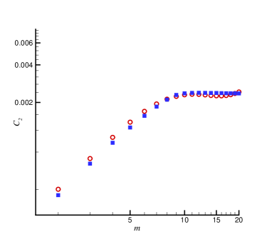
FIG. 5.: Logarithmic plot of the second moment of the height-difference versus $m$, for the actual data (circles) and the samples regenerated by the kernel method (squares). The corresponding time series are plotted in Fig. 4.

The Cascade of Information from Large to Small Time Scales

We would argue that if long-range, nondecaying correlations do exist in the time series, then one may not be able to use the above reconstruction method for analyzing them because, as is well-known, the correlations in a Markov process decay exponentially. Aside from the fact that even in such cases the method described above provides an unambiguous way of distinguishing healthy subjects from those with CHF, which we believe is more effective than simply analyzing the data to see what type of correlations may exist in the data (see below), we argue that the nondecaying correlations do not, in fact, pose any limitations to the fundamental ideas and concepts of the reconstruction method described above.

The reason is that, even if the above reconstruction method fails to describe long-range, nondecaying correlations in the data, one can still analyze the data based on the same method by invoking an important result recently pointed out by several groups.^20,21,23-25 They studied the evolution of the PDF of several stochastic properties of turbulent free jets, and rough surfaces. They pointed out that the conditional PDF of the increments of a stochastic field, such as the increments in the velocity field in the turbulent flow or heights fluctuations of rough surface, satisfies the CK equation even if the velocity field or the height function itself contains long-range, nondecaying correlations. This enabled them to derive a FP equation for describing the systems under study. Hence, one has a way of analyzing correlated stochastic time series or data in terms of the corresponding FP and CK equations. We now describe the conditions under which such a formulation can be utilized.

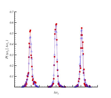
FIG. 6.: Test of Chapman-Kolmogorov equation for $\Delta x_{1}=-0.42$, $\Delta x_{1}=0$ and $\Delta x_{1}=0.42$. The solid and open symbols represent, respectively, the directly-evaluated PDF and the one obtained from Eq. (1). The PDFs are shifted in the horizontal directions for clarity. Values of $\Delta x$ are measured in units of the standard deviation of the increments. The time scales $\tau_{1}$, $\tau_{2}$ and $\tau_{3}$ are $10$, $30$, and $20$, respectively.

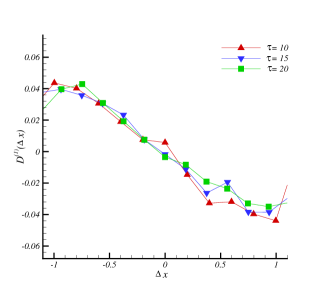
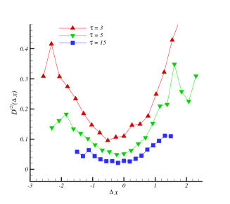
FIG. 7.: The drift and diffusion coefficients $D^{(1)}(\Delta x)$ and $D^{(2)}(\Delta x)$, estimated from Eq. (3) for a healthy subject, follow linear and quadratic behavior, respectively.

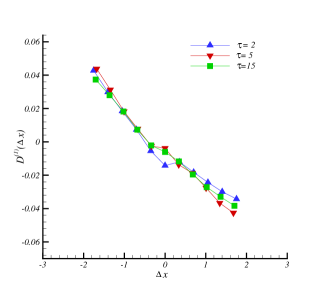
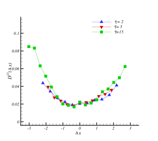
FIG. 8.: The drift and diffusion coefficients $D^{(1)}(\Delta x)$ and $D^{(2)}(\Delta x)$ are estimated from the Eq. (3) for typical patients with heart failure, and follow linear and quadratic behavior, respectively.

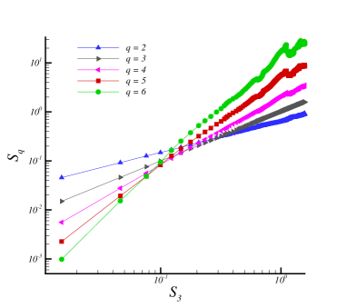
FIG. 9.: Generalized scaling analysis of a typical healthy subject. Structure functions $S_{q}$ are displayed versus $S_{3}$ in log-log scale.

In such cases, one computes the Kramers-Moyal (KM) coefficients for the increments of interbeat intervals fluctuatations, $\Delta x(\tau)=x(t+\tau)-x(t)$, rather than the time series $x(t)$ itself. One then checks whether the first and second KM coefficients that represent, respectively, the drift and diffusion coefficients in a FP equation, have well-defined and finite values, while the third- and fourth-order KM coefficients are small. According to the Pawula‘s theorem,²⁴ the KM expansion,

$$\frac{\partial}{\partial t}P(x,t|x_{0},t_{0})=\sum_{k=1}^{\infty}\left(-\frac{\partial}{\partial x}\right)^{k}\left[D^{(k)}(x,t)P(x,t|x_{0},t_{0})\right]\;,$$ (12)

can be truncated after the second (diffusive) term, provided that the third- and fourth-order coefficient $D^{(4)}$ vanish, or are very small compared with the first two coefficients. If so, which is often the case, then the KM expansion, Eq. (12), reduces to a FP evolution equation. In that case, a FP equation is numerically constructed by computing its drift and diffusion coefficients for the PDF $P(\Delta x,\tau)$ which, in turn, is used to gain information on evolution of the shape of the PDF as a function of the time scale $\tau$. In essence, if the first two KM coefficients are found to have numerically-meaningful values (i.e., not very small), while the third and higher coefficients are small compared with the first two coefficients, the above reconstruction method - Eqs. (2)-(5) - are used for the increments of the times series, rather than the time series itself.

Therefore, carrying out the same type of computations described above, but now for the increaments $\Delta x(t)$, the following results are computed for the healthy subjects,²⁸

$$D^{(1)}(\Delta x,\tau)=-(3\Delta x+0.46)\times 10^{-2}\;,$$ (13)

$$D^{(2)}(\Delta x,\tau)=\left[\left(1+11\tau^{-1}\right)(\Delta x)^{2}+\left(5.7+28.7\tau^{-1}\right)\right]\times 10^{-2}\;,$$ (14)

whereas for the patients with CHF we obtain,

$$D^{(1)}(\Delta x,\tau)=-(1.3\Delta x+0.18)\times 10^{-2}\;,$$ (15)

$$D^{(2)}(\Delta x,\tau)=\left[\left(5+5\tau^{-1}\right)(\Delta x)^{2}+\left(13+66\tau^{-1}\right)\right]\times 10^{-3}\;.$$ (16)

Estimates of the above coefficients are less accurate for large values of $\Delta x$. Also computed are the average of the coefficients $D^{(1)}$ and $D^{(2)}$ for the entire set of the healthy subjects, as well as those with CHF. Moreover, $D^{(4)}$ is about $\frac{1}{10}D^{(2)}$ for the healthy subjects, and about $\frac{1}{20}D^{(2)}$ for those with CHF. Therefore, the KM expansion can indeed be truncated beyond the second term, and the FP formulation is numerically justified.

Equations (13)-(16) state that the drift coefficients for the healthy subjects and those with CHF have the same order of magnitude, whereas the diffusion coefficients for the given $\tau$ and $\Delta x$ differ by about one order of magnitude. This points to a relatively simple way of distinguishing the two classes of the subjects. Moreover, the $\tau$-dependence of the diffusion coefficient for the healthy subjects is stronger than that of those with CHF (in the sense that the numerical coefficients of the $\tau^{-1}$ are larger for the healthy subjects). These are shown in Figures 7 and 8. Note also that these results are consistent with those presented earlier for the time series $x(t)$ itself, in terms of distinguishing the two classes of patients through their different drift and diffusion coefficients.

The strong $\tau-$dependence of the diffusion coefficient $D^{(2)}$ for the healthy subjects indicates that the nature of the PDF of their increments $\Delta x$ for given $\tau$, i.e., $P(\Delta x,\tau)$, is intermittent, and that its shape should change strongly with $\tau$. However, for the patients with CHF the PDF is not so sensitive to the change of the time scale $\tau$, hence indicating that the increments’ fluctuations for these patients is not intermittent.

The Extended Self-Similarity of Interbeat Intervals in Human Subjects

Let s look at another computational method for distinguishing healthy subjects from CHF patients. The method is based on the concept of extended self-similarity (ESS) of a time series. This concept is particularly useful if the time series for interbeat fluctuations (or other types of time series) do not, as is often the case, exhibit scaling over a broad interval. In such cases, the time interval in which the structure function of the time series, i.e.,

$$S_{q}(\tau)=\langle|x(t+\tau)-x(t)|^{q}\rangle\;,$$ (17)

behaves as

$$S_{q}(\tau)\sim\tau^{\xi_{q}}\;,$$ (18)

is small, in which case the existence of scale invariance in the data can be questioned. However, instead of rejecting outright the existence of scale invariance, one must first explore the possibility of the data being scale invariance via the concept of ESS.

The ESS is a powerful tool for checking non-Gaussian properties of data,^31,32 and has been used extensively in research on turbulent flows. Indeed, when analyzing the interbeat time series for human subjects (and other types of time series), one can, in addition to the $\tau$-dependence of the structure function, compute a generalized form of scaling using the ESS concept. In many cases, when the structure functions $S_{q}(\tau)$ are plotted against a structure function of a specific order, say $S_{3}(\tau)$, an extended scaling regime is found according to,^31,32

$$S_{q}(\tau)\sim S_{3}(\tau)^{\zeta_{q}}\;.$$ (19)

Clearly, meaningful results are restricted to the regime where $S_{3}$ is monotonic. For any Gaussian process the exponents $\zeta_{q}$ follow a simple equation,

$$\zeta_{q}=\frac{1}{3}q\;.$$ (20)

Therefore, systematic deviation from the simple scaling relation, Eq. (20), should be interpreted as deviation from Gaussianity. An additional remarkable property of the ESS is that it holds rather well even in situations when the ordinary scaling does not exit, or cannot be detected due to small scaling range, which is the case for the data analyzed here.

Using the ESS concept, we analyzed³³ the fluctuations in human heartbeat rates of healthy subjects and those with CHF, analyzed earlier with the reconstruction method. The results are shown in Figure 9. For a typical healthy subject an improved scaling behavior of the time series is indicated by the ESS. In Figure 10 the computed scaling exponents $\zeta_{q}$ of the structure functions are plotted against the order $q$. A mono-fractal time series corresponds to linear dependence of $\zeta_{q}$ on $q$, whereas for a multifractal time series $\zeta_{q}$ depends nonlinearly on $q$. The constantly changing curvature of the computed $\zeta_{q}$ for the healthy subjects suggests multifractality of their corresponding time series. In contrast, $\zeta_{q}$ is essentially linear for the patients with CHF, indicating mono- or simple fractal behavior.

It is well-known that the moments with $q<1$ and $q>1$ are related, respectively, to the frequent and rare events in the time series.^30,31 Thus, for the data considered here one may also be interested in the frequent events in the interbeats. In Figure 11 we show the results for the moment $q=0.1$ against a third-order structure function for healthy subjects and those with CHF. There are two interesting features in Figure 11. First, the starting point of $S_{0.1}(\tau)$ versus $S_{3}(\tau)$ is different for the data for healthy subjects and patients with CHF. To determine the distance form the origin, we define,³⁴

$$T(\tau=1)=[S^{2}_{0.1}(\tau=1)+S^{2}_{3}(\tau=1)]^{1/2}\;.$$ (21)

The second important feature of Figure 11 is that there is a well-defined $\tau^{*}$ beyond which the plot of $S_{0.1}(\tau)$ versus $S_{3}(\tau)$ is multi-valued. One can estimate $\tau^{*}$ by checking when $S_{3}(\tau)>S_{3}(\tau+1)$. Moreover, if we define $T(\tau^{*})$ by,

$$T(\tau^{*})=[S^{2}_{0.1}(\tau^{*})+S^{2}_{3}(\tau^{*})]^{1/2}\;,$$ (22)

then, there is a time scale $\tau^{*}$ such that the values of the third moment before and after $\tau^{*}$ are almost the same. Thus, the quantity $\tau^{*}$ plays a role of a local mirror on the time axis. In other words, locally, $S_{3}(\tau)$ for $\tau<\tau^{*}$ and $\tau>\tau^{*}$ has almost the same value. In Figure 11, we show the time scale $\tau^{*}$ and, therefore, indicate that values of $T(\tau=1)$ and $T(\tau^{*})$ of the interbeat fluctuations of the healthy subjects and patients with CHF are different.

Table 1 presents the computed values of $T_{1}=T(\tau=1)$ for both healthy subjects and those with CHF. To compute the results, we first rescaled the data sets by their standard deviation and, therefore, the $T_{1}$ values are dimensionless. The average value of $T_{1}$ for the healthy subjects is, $\bar{T}(\tau=1)\simeq 0.5848$, with its standard deviations being, $\sigma\simeq 0.065$. The corresponding values for the daytime records of the patients with CHF are, $\bar{T}(\tau=1)\simeq 0.5077$ and $\sigma\simeq 0.03$, respectively. Therefore, on average, healthy subjects possess $T_{1}$ values that are greater than those of the patients with CHF. However, note that $T_{1}$ for the various data sets do not have large enough differences to be able to distinguish unambiguously the data sets. Indeed, as Table 1 indicates, three of the data sets (belonging to the day- and nighttime records of one healthy subject, with the third one belonging to the daytime of another healthy subject) overlap.

To develop a more definitive criterion for distinguishing the data for various subjects, we compute values of $T(\tau^{*})$. The results are listed in Table 2. It is evident that, in this case, there is no overlap in the data sets. Indeed, the $T(\tau^{*})$ values for the healthy subjects are larger, by a factor of about 3, than those for the patients with CHF, hence providing an unambiguous way of distinguishing the data sets for healthy subjects and those with CHF.

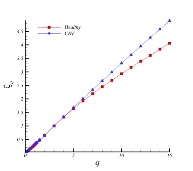
FIG. 10.: The plot of $\zeta_{q}$ versus $q$, which has a linear dependence on $q$ for CHF subjects, but a nonlinear dependence on $q$ for the healthy subjects.

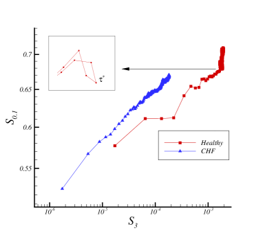
FIG. 11.: Plot of $S_{0.1}$ against $S_{3}(\tau)$ for a healthy and one with CHF. The results indicate that the starting points are different for healthy subjects and those with CHF. Moreover, for the both data set there is a well-defined $\tau^{*}$ at which $S_{3}(\tau)>S_{3}(\tau+1)$.

TABLE I.: Values of $T_{1}$ for the healthy subjects (day time and night time ) and those with CHF.

$Healthy$	$CHF$
0.658	0.557
0.672	0.565
0.614	0.539
0.605	0.526
0.583	0.512
0.581	0.493
0.576	0.492
0.558	0.481
0.494	0.469
0.480	0.443

TABLE II.: Values of the $T(\tau^{*})$ for the healthy subjects (day time and night time) and for those with CHF.

$Healthy$	$CHF$
3.08	0.741
2.68	0.714
2.34	0.685
1.92	0.681
1.86	0.675
1.42	0.632
1.40	0.573
1.22	0.728
1.20	0.552
1.15	0.465

Comparison with other Methods

Stanley and colleagues^{5,13,19,26,27,38} and other^35-37 analyzed the type of data that we consider in this review by different methods. Their analyses indicate that there may be long-range correlations in the data, characterized by self-affine fractal distributions, such as the fractional Brownian motion, the power spectrum of which is given by,

$$S(f)\sim f^{-(2H+1)}\;,$$ (23)

where $H$ is the Hurst exponent that characterizes the type of the correlations in the data. Thus, healthy subjects are distinguished from those with CHF in terms of the type of correlations that might exist in the data: negative or antipersistent correlations in the increments for $H<1/2$, as opposed to positive or persistent correlations for $H>1/2$, and Brownian motion for $H=1/2$. While this is an important and interesting result, it can also be ambiguous and not very precise. For example, suppose that the analysis of two time series yields two values of $H$, one slightly larger and the second one slightly smaller than $1/2$. Then, 2. It s thus difficult to state with confidence that the two times series are really distinct.

The reconstruction method described earlier analyzes the data in terms of the Markov processes properties. As a result, it distinguishes the data for healthy subjects from those with CHF in terms of the differences between an FP equation s drift and diffusion coefficients. Such differences are typically very significant and, therefore, provide, in our view, an unambiguous way of understanding the differences between the two groups of the subjects, including for those series for which the Hurst exponents are only slightly different. In addition, the computational approach described in this review provides an unambiguous way of reconstructing the data, hence providing a means of predicting the behavior of the data over periods of time that are on the order of their Markov time scales.

Although it remains to be tested, we believe that, together, all the computational methods that have been described in this review are more sensitive to small differences between the data for the two groups of the subjects and, therefore, might eventually provide a diagnostic tool for early detection of CHF in patients.

Finally, the computational approaches described in this review are quite general, and may be used for analyzing times series that represent the dynamics of completely unrelated phenomena. For example, we have used the concepts of Markov processes and extended self-similarity to develop³⁴ a method for providing short-term alerts for moderate and large earthquakes, as well as making predictions for the price of oil.³⁹

Biographies:

Mohammad Reza Rahimi Tabar is Associate Professor of Physics at the Sharif University in Tehran, Iran. His main research areas are conformal field theory, disordered systems, statistical theory of turbulence, stochastic processes, seismic activity, and wave localization. He can be reached at rahimitabar$@$sharif.edu.

Fatemeh Ghasemi is a post-doctoral fellow at Institute for Studies in Theoretical Physics and Mathematics in Tehran, Iran. Her main research interests are stochastic processes, analysis of time series and of rough surfaces, and seismic activity. She can be reached at
f$\_$ghasemi$@$mehr.sharif.edu.

Joachim Peinke is a Professor at the University of Oldenburg in Germany. His main research areas are turbulence, econophysics, pattern formation in nematic liquid crystals, stochastic processes, and development of various sensors. He can be reached at peinke$@$uni-oldenburg.de.

Rudolf Friedrich is a Professor at the University of Münster, Germany. His main research areas are turbulence, econophysics, pattern formation in nematic liquid crystals, and stochastic processes. He can be reached at fiddir$@$uni-muenster.de .

Kamran Kaviani is Assistant Professor of Physics at Alzahra University, in Tehran, Iran. His main research are stochastic processes and field theory. He can be reached at kaviani$@$yahoo.com.

Fatemeh Taghavi is a Ph.D. student in physics at Iran University of Science and Technology in Tehran, Iran. Her main research areas are stochastic processes and field theory. She can be reached at f$\_$taghavi$@$iust.ac.ir.

Sara Sadeghi is a Ph.D. student in physics at Sharif University in Tehran, Iran. Her main reseach area is analysis of complex systems. She can be reached at s$\_$sara2001@yahoo.com.

Golnoosh Bizhani is pursuing her M.Sc. degree in physics at Sharif University in Tehran, Iran. Her main reseach area is analysis of complex systems. She can be reached at
golnoosh$\_$bizhani$@$yahoo.com.

Muhammad Sahimi is Professor of Chemical Engineering and Materials Science, and NIOC Professor of Petroleum Engineering at the University of Southern California in Los Angeles. His main research areas are atomistic simulation of nanostructured materials, modeling of large-scale porous media, wave propagation in heterogeneous media, and analysis of stochastic processes. He can be reached at moe$@$iran.usc.edu.

REFERENCES

- [1] M.F. Shlesinger, ”Behavioral-Independent Features of Complex Heartbeat Dynamics,” Ann. NY Acad. Sci. 504, 214 (1987).
- [2] J.B. Bassingthwaighte, L.S. Liebovitch, and B.J. West, Fractal Physiology, Oxford University Press, New York (1994).
- [3] M. Malik and A.J. Camm (eds.), Heart Rate Variability, Futura, Armonk, New York (1995).
- [4] M. Kobayashi and T. Musha, ” Fluctuation of Heartbeat Period,” IEEE Trans. Biomed. Eng. 29, 456 (1982)
- [5] J.M. Hausdorff, P.L. Purdon, C.-K. Peng, Z. Ladin, J.Y. Wei, and A.L. Goldberger, ”Fractal Dynamics of Human Gait- Stability of Long-Range Correlations in Stride Interval Fluctuations,” J. Appl. Physiol. 80, 1448 (1996).
- [6] S.B. Lowen, L.S. Liebovitch, and J.A. White, Phys. Rev. E 59, 5970 (1999).
- [7] Y. Yamamoto, R.L. Hughson, J.R. Sutton, C.S. Houston, A. Cymerman, E.L. Fallen, and M.V. Kamath, ”An Indication of Deterministic Chaos in Human Heart Rate Variability at Simulated Extreme Altitude,” Biol. Cybern. 69, 205 (1993).
- [8] J.K. Kanters, N.H. Holstein-Rathlou, and E. Agner, “Lack of Evidence for Low-Dimensional Chaos in Heart Rate Variability,” J. Cardiovasc. Electrophysiol. 5, 128 (1994).
- [9] J. Kurths, A. Voss, P. Saparin, A. Witt, H.J. Kleiner, and N. Wessel, “Complexity Measures for the Analysis of Heart Rate Variability,” Chaos 5, 88 (1995).
- [10] P.Ch. Ivanov, M.G. Rosenblum, C.-K. Peng, J. Mietus, S. Havlin, H.E. Stanley, and A. L. Goldberger, ”Scaling Behaviour of Heartbeat Intervals Obtained by Wavelet-Based Time-Series Analysis,” Nature 383, 323 (1996).
- [11] G. Sugihara, W. Allan, D. Sobel, and K.D. Allan, “Nonlinear Control of Heart Rate Variability in Human Infants,” Proc. Natl. Acad. Sci. USA 93, 2608 (1996).
- [12] C.-S. Poon and C.K. Merrill, “Decrease of Cardiac Chaos in Congestive Heart Failure,” Nature 389, 492 (1997).
- [13] P.Ch. Ivanov, L.A.N. Amaral, A.L. Goldberger, S. Havlin, M.G. Rosenblum, Z. Struzik, and H.E. Stanley, “Multifractality in Human Heartbeat Dynamics,” Nature 399, 461 (1999).
- [14] M. Mackey and L. Glass, “Oscillation and Chaos in Physiological Control Systems,” Science 197, 287 (1977).
- [15] M.M. Wolf, G.A. Varigos, D. Hunt, and J.G. Sloman, ”Sinus Arrhythmia in Acute Myocardial Infarction,” Med. J. Australia 2, 52 (1978).
- [16] R.I. Kitney and O. Rompelman, The Study of Heart-Rate Variability, Oxford University Press, London (1980).
- [17] S. Akselrod, D. Gordon, F.A. Ubel, D.C. Shannon, A.C. Barger, and R.J. Cohen, ”Power Spectrum Analysis of Heart Rate Fluctuation: a Quantitative Probe of Beat-to-Beat Cardiovascular Control,” Science 213, 220 (1981).
- [18] C.-K. Peng, S. Havlin, H.E. Stanley, and A.L. Goldberger, ”Quantification of Scaling Exponents and Crossover Phenomena in Nonstationary Heartbeat Time Series,” Chaos 5, 82 (1995)
- [19] Y. Ashkenazy, P.Ch. Ivanov, S. Havlin, C.-K. Peng, A.L. Goldberger, and H.E. Stanley, ”Magnitude and Sign Correlations in Heartbeat Fluctuations,” Phys. Rev. Lett. 86, 1900 (2001).
- [20] R. Friedrich and J. Peinke, ”Description of a Turbulent Cascade by a Fokker-Planck Equation,” Phys. Rev. Lett. 78, 863 (1997).
- [21] J. Davoudi and M.R. Rahimi Tabar, ”Theoretical Model for the Kramers-Moyal Description of Turbulence Cascades,” Phys. Rev. Lett. 82, 1680 (1999).
- [22] G.R. Jafari, S.M. Fazlei, F. Ghasemi, S.M. Vaez Allaei, M.R. Rahimi Tabar, A. Iraji Zad, and G. Kavei, ”Stochastic Analysis and Regeneration of Rough Surfaces,” Phys. Rev. Lett. 91, 226101 (2003).
- [23] R. Friedrich, J. Peinke, and C. Renner, ”How to Quantify Deterministic and Random Influences on the Statistics of the Foreign Exchange Market,” Phys. Rev. Lett. 84, 5224 (2000).
- [24] M. Siefert, A. Kittel, R. Friedrich, and J. Peinke, ”On a Quantitative Method to Analyze Dynamical and Measurement Noise,” Eur. Phys. Lett. 61, 466 (2003).
- [25] M. Ragwitz and H. Kantz, ”Indispensable Finite Time Corrections for Fokker-Planck Equations from Time Series Data,” Phys. Rev. Lett. 87, 254501 (2001).
- [26] P.Ch. Ivanov, A. Bunde, L.A.N. Amaral, S. Havlin, J. Fritsch-Yelle, R.M. Baevsky, H.E. Stanley, and A.L. Goldberger, ”Sleep-Wake Differences in Scaling Behavior of the Human Heartbeat: Analysis of Terrestrial and Long-Term Space Flight Data,” Europhys. Lett. 48, 594 (1999).
- [27] Y. Ashkenanzy, P.Ch. Ivanov, L. Glass, A.L. Goldberger, V. Schulte-Frohlinde, and H.E. Stanley, ”Noise Effects on the Complex Patterns of Abnormal Heartbeats,” Phys. Rev. Lett. 87, 068104/1-068104/4 (2001).
- [28] F. Ghasemi, J. Peinke, M. Sahimi, and M.R. Rahimi Tabar, “Regeneration of Stochastic Processes: An Inverse Method,” Eur. Phys. J. B 47, 411 (2005).
- [29] F. Ghasemi, J. Peinke, M.R. Rahimi Tabar, and M. Sahimi, “Statistical Properties of the Interbeat Interval Cascade in Human Hearts,” Int. J. Mod. Phys. C, in press (2005).
- [30] . Kuusela, ”Stochastic Heart-Rate Model can Reveal Pathologic Cardiac Dynamics,” Phys. Rev. E 69, 031916/1-031916/5 (2004).
- [31] R. Benzi, L. Biferale, S. Ciliberto, M.V. Struglia, and R. Tripiccione, ”Scaling Property of Turbulent Ows,” Physica D 96, 162 (1996).
- [32] A. Bershadskii and K.R. Sreenivasan, ”Extended Self-Similarity of the Small-Scale Cosmic Microwave Background Anisotropy,” Phys. Lett. A 319, 21 (2003).
- [33] F. Ghasemi, K. Kaviani, M. Sahimi, M.R. Rahimi Tabar, F. Taghavi, S. Sadeghi, and G. Bijani, “The Extended Self-Similarity of Interbeat Intervals in Human Subjects,” preprint.
- [34] M.R. Rahimi Tabar, M. Sahimi, K. Kaviani, M. Allamehzadeh, J. Peinke, M. Mokhtari, M. Vesaghi, M.D. Niry, F. Ghasemi, A. Bahraminasab, S. Tabatabai, and F. Fayazbakhsh, ”Dynamics of the Markov Time Scale of Seismic Activity May Provide a Short-Term Alert for Earthquakes,” Arxiv: Physics/0510043.
- [35] R.G. Turcott and M.C. Teich, ”Fractal Character of the Electrocardiogram: Distinguishing Heart-Failure and Normal Patients,” Ann. Biomed. Eng. 24, 269 (1996).
- [36] L.A. Lipsitz, J. Mietus, G.B. Moody, and A.L. Goldberger, ”Spectral Characteristics of Heart Rate Variability before and During Postural Tilt. Relations to Aging and Risk of Syncope,” Circulation 81, 1803 (1990).
- [37] Iyengar N, Peng CK, Morin R, Goldberger AL, Lipsitz LA. , ”Age-related Alterations in the Fractal Scaling of Cardiac Interbeat Interval Dynamics,” Am. J. Physiol. 271, R1078 (1996).
- [38] P.Ch. Ivanov, L.A.N. Amaral, A.L. Goldberger, and H.E. Stanley, ”Stochastic Feedback and the Regulation of Biological Rhythms,” Europhys. Lett. 43, 363 (1998).
- [39] F. Ghasemi, M. Sahimi, J. Peinke, R. Friedrich, and M.R. Rahimi Tabar, “The Kramers-Moyal Expansion and Langevin Equation for the Stochastic Fluctuations in the Oil Price,” Phys. Rev. Lett., submitted.