Quantifying the information transmitted in a single stimulus

Abstract

Shannon mutual information provides a measure of how much information is, on average, contained in a set of neural activities about a set of stimuli. It has been extensively used to study neural coding in different brain areas. To apply a similar approach to investigate single stimulus encoding, we need to introduce a quantity specific for a single stimulus. This quantity has been defined in literature by four different measures, but none of them satisfies the same intuitive properties (non-negativity, additivity), that characterize mutual information. We present here a detailed analysis of the different meanings and properties of these four definitions. We show that all these measures satisfy, at least, a weaker additivity condition, i.e. limited to the response set. This allows us to use them for analysing correlated coding, as we illustrate in a toy-example from hippocampal place cells.

1 Information theory and mutual information

Information theory [1] provides a natural mathematical framework to answer the question: how much information is contained in the neural patterns. Usually, in an experiment, we choose a controlled sample of stimuli ${\cal S}$, and we record the elicited neural responses $r\in{\cal R}$ when one stimulus $s\in{\cal S}$ is repeatedly presented with a known a priori probability $p(s)$. From these data, we can estimate the corresponding joint probabilities $p(r,s)$ and the probability distribution of responses averaged over the stimuli $p(r)$; and then compute the mutual information:

$$I({\cal S};{\cal R})=\sum_{s\in{\cal S},r\in{\cal R}}p(r,s)\ \log_{2}\left[\frac{p(r,s)}{p(r)p(s)}\right]=\sum_{s\in{\cal S},{r\in{\cal R}}}p(s)p(r|s)\ \log_{2}\left[\frac{p(r|s)}{p(r)}\right],$$ (1)

(with conditional probability $p(r|s)=p(r,s)/p(s)$ according to Bayes’ rule) or, equivalently, introducing the entropy of a probability distribution: $H({\cal R})=-\sum_{r\in{\cal R}}p(r)\log_{2}p(r)$,

$$I({\cal S};{\cal R})=H({\cal R})-H({\cal R}|{\cal S})=\sum_{s\in{\cal S}}p(s)[H({\cal R})-H({\cal R}|s)]$$ (2)

where $H({\cal R}|{s})\equiv\sum_{s\in{\cal S}}p(s)H({\cal R}|{\cal S})$ is the conditional entropy.

Mutual information summarizes the average amount of knowledge we gain about the stimulus by observing neural responses (or vice-versa); e.g.: in the trivial case, they are completely uncorrelated, $p(r,s)=p(r)p(s)$ and $I=0$.

Mutual information has some mathematical properties that agree to our intuitive notion of information. In particular, we expect that any observation does not decrease the knowledge we have about the system. So, mutual information has to be positive, as it can be easily shown starting from Shannon definition. Furthermore, if we observe the response from two different neurons or two different aspects of single unit response, $\{{\cal R}^{1},{\cal R}^{2}\}$, the overall information about the stimulus set $I(\{{\cal R}^{1},{\cal R}^{2}\};{\cal S})$ is the sum of the information contained in the first response ${\cal R}^{1}$, plus the information we gain by reading the second response ${\cal R}^{2}$ given we know ${\cal R}^{1}$ (chain rule), i.e.:

$$I(\{{\cal R}^{1},{\cal R}^{2}\};{\cal S})=I({\cal R}^{1};{\cal S})+I({\cal R}^{2};{\cal S}|{\cal R}^{1})$$ (3)

Relationship (3) may be used to investigate the independence of coding in cell population or in presence of multiple response features [4]. For example, if $\{{\cal R}^{1},{\cal R}^{2}\}$ encode different features of the stimulus independently, then the information they convey about the stimulus has to be the sum of the information conveys separately, i.e. $I(\{{\cal R}^{1},{\cal R}^{2}\},{\cal S}\})=I({\cal R}^{1},{\cal S})+I({\cal R}^{2},{\cal S})$. Thus, by evaluating this information (or synergy function [4]) we can quantitatively estimate the different contributions to the stimulus encoding from the different response features. Note that this additivity property directly relies on the validity of the chain rule (3). Similarly, due to its symmetric form, we can express the chain rule in terms of two different stimuli features (e.g. color and shape in visual stimuli) $\{{\cal S}^{1},{\cal S}^{2}\}$

$$I({\cal R};\{{\cal S}^{1},{\cal S}^{2}\})=I({\cal R};{\cal S}^{1})+I({\cal R};{\cal S}^{2}|{\cal S}^{1})$$ (4)

2 Stimulus specific information

In many cases it may be interesting to know which stimulus contained more information in a given set [5, 6], or investigate how a single stimulus is encoded in terms of different response features. In his original formulation, Shannon did not provide any insights about how much information can be carried by a single symbol, such as a single stimulus in our case. After Shannon’s seminal work, many definitions of one-symbol specific information have been introduced, usually referred as stimulus specific information in the neural processing context. Ideally, stimulus specific information should be proper information in a mathematical sense (non-negative, additive) and give mutual information when averaged over the stimulus set. Four different alternative definitions have been proposed in literature. We give here a detailed analysis of their features and different meanings. In particular, we investigate the different roles of stimulus and response regarding additivity rules, Eqs.(3, 4), (Section 3) and show a possible application (Section 4). In Table 1 we summarize the main features of these four quantities.

We conclude that there is no “fully” satisfactory definition of this quantity, in the sense that no one of these definitions shares all mathematical properties of Shannon mutual information, which is so appealing from the application point of view; but each of them can be used to investigate different aspects of single stimulus information transmission.

Stimulus specific surprise

Originally proposed by Fano [7], this definition can be immediately inferred from Eq. (1), simply taking the single stimulus contribution to the sum:

$$I_{1}(s)=Surprise(s)=\sum_{r\in{\cal R}}p(r|s)\log_{2}\frac{p(r|s)}{p(r)}$$

This quantity measures the deviation (also called Kullback-Leibler distance) between the marginal distribution $p(r)$ and conditional probability distribution $p(r|s)$. It clearly averages to the mutual information, i.e. $\sum_{s\in{\cal S}}p(s)I_{1}(s)=I({\cal S};{\cal R})$, and it is always non-negative: $I_{1}(s)\geq 0$ for $s\in{\cal S}$. Furthermore it is the only positive decomposition of the mutual information (for the proof, see Appendix 2 in Ref. [11]). Since $I_{1}(s)$ is large when $p(r|s)$ dominates in the regions where $p(r)$ is small, i.e. in presence of surprising events, this quantity is often referred as “stimulus specific surprise” or simply “surprise”. Surprise lacks additivity, and this causes many difficulties when we want to apply it to a sequence of observations. Despite this main drawback, specific surprise has been widely used in neural coding literature (see for example [8, 9, 10]).

Stimulus specific information

An entropy based definition has been proposed by De Weese and Meister [11] and it may be derived from Eq. (2), extracting the single stimulus contribution from the sum:

$$I_{2}(s)=H({\cal R})-H({\cal R}|s)=-\left[\sum_{r\in{\cal R}}p(r)\log_{2}p(r)-p(r|s)\log_{2}p(r|s)\right]$$

Here, information is identified with the reduction of entropy between marginal distribution $p(r)$ and conditional probability $p(r|s)$. This quantity captures the reliability of the neural response for a given stimulus. Indeed, it expresses the difference of uncertainty between the a priori knowledge of the response set, $H({\cal R})$, and after stimulus presentation $H({\cal R}|s)$. A stimulus characterized by highly predictable responses has a large $I_{2}(s)$ value. This means that we can easily predict a response when we know the stimulus, but not necessarily vice-versa.

As shown in [11], this is the only decomposition of mutual information that is also additive, but, unlike mutual information, it can assume negative values.

Note that any weighted combination of $I_{1}$ and $I_{2}$ averages to mutual information, and it can represent a possible definition of stimulus specific information. Thus, we have an infinite number of plausible choices for a stimulus-dependendent decomposition of mutual information. But, as mentioned above, only $I_{1}$ is always non-negative and for $I_{2}$ only the chain rule 4 is fulfilled.

Stimulus specific information (SSI) (2)

More recently Butts [13] introduced a new definition, which emphasizes the causal relationship between stimulus and response in neural processing:

$$I_{3}(s)=SSI(s) = \sum_{r\in{\cal R}}p(r|s)I_{2}(r)=\sum_{r\in{\cal R}}p(r|s)\left[H({\cal S})-H({\cal S}|r)\right]$$

$$= H({\cal S})-\sum_{r\in{\cal R}}p(r|s)H({\cal S}|r)$$

where $I_{2}(r)$ is one-symbol specific information applied to a single neural response: $I_{2}(r)=H({\cal S})-H({\cal S}|r)$. This measure represents the average reduction of uncertainty (difference of entropy) after an observation of the response given the stimulus, or, in other words, the stimulus-conditioned average of the response-specific information $I_{2}(r)$. So, if one stimulus is characterised by a very informative response, in the sense of $I_{2}(r)$ (such as responses that almost completely determine the stimulus), it results in a large value of $I_{3}$.

Stimulus information density $I_{l}$

A fourth definition has been proposed by Bezzi et al. [12] in the framework of position-encoding in hippocampal formation.

$$I_{4}(s)=I_{l}(s) = I({\cal R};\{s,\bar{s}\})=$$ (5)

$$= \sum_{r\in{\cal R}}p(s)p(r|s)\log_{2}\left[\frac{p(r|s)}{p(r)}\right]+p(\bar{s})p(r|\bar{s})\log_{2}\left[\frac{p(r|\bar{s})}{p(r)}\right],$$ (6)

where $\bar{s}$ is the complementary set of $s$, i.e. $\bar{s}\equiv\bigcup_{s^{\prime}\in{\cal S},s^{\prime}\neq s}s^{\prime}$ (with $s\bigcup\bar{s}={\cal S}$). In other words, we partition the set of stimuli into two subsets, one containing the stimulus $s$ only and the complementary set composed by all the other stimuli, then we compute the average mutual information using these two stimuli set. This is a measure of how well we can distinguish between the single stimulus $s$ and all the others observing the neural response ${\cal R}$. $I_{4}$ is an actual mutual information, thus it is positive and additive (this last condition holds only for a very particular choice of the stimuli, see below), but it does not average to mutual information of the whole stimulus set (i.e. $\sum_{s\in{\cal S}}p(s)I_{4}(s)\neq I({\cal S};{\cal R})$).

This quantity has a simple relationship with specific surprise $I_{2}$ for very unlikely stimuli $p(s)\ll 1$. Indeed, expanding Eq. (6) for $p(s)\ll 1$ we get:

$$I_{l}(s) = p(s)\sum_{r\in{\cal R}}p(r|s)\log_{2}\left[\frac{p(r|s)}{p(r)}\right]+\mathcal{O}({p(s)^{2}})$$ (7)

that corresponds to $p(s)I_{1}(s)$. This expression has two consequences: it supplies an additional theoretical justification to specific surprise and assures that if we have a large set of stimuli characterized by $p(s)\ll 1$ for each ${s\in{\cal S}}$ the sum of the local information converges to the average mutual information.

Definition	Positive	Chain rule	Chain rule	Average MI
	definite	(Responses)	(Stimuli)
$I_{1}$ Surprise	Yes	Yes	No	Yes
$I_{2}$	No	Yes	Yes	Yes
$I_{3}$	No	Yes	No	Yes
$I_{4}$	Yes	Yes	Yes/No	No

Table 1: Main properties of the four definitions of stimulus specific information.

3 A weaker additivity condition

Among the above four definitions for stimulus specific information, only $I_{2}$ is additive (obeying Eqs. (3, 4)) [11]. But, despite not being additive in a rigorous sense, the other three quantities still fulfill relationship (3), but not (4), or in other words, they are additive limited to the response set. This results in a weaker additivity property, which may still be used for investigating how different features of the response encode a single stimulus, such as testing independence (see Section 4 for an example). We should remark that due to the different meanings of the four definitions, this analysis can give contradictory results depending on the measure chosen. A special case is represented by $I_{4}$, because it is a proper mutual information (with a particular choice of stimulus set), then we expect it to be additive in terms of stimuli, too. But, $I_{4}(s)$ requires an additional constraint: the two subsets partition, $\{s,\bar{s}\}$, of stimulus set ${\cal S}$. This last condition cannot be preserved in general for the chain rule, Eq. (4) [12].

4 Stimulus specific information in hippocampal place cells

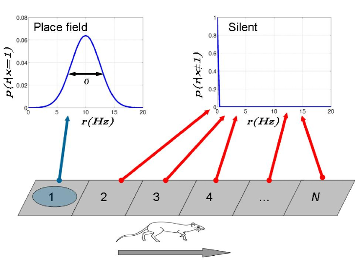
Figure 1: A rat running in linear track (unidirectional). Position in the track is binned, in $N$ spatial bins. Conditional probability distribution for a place cell: $x_{1}$, place field (top, left) and $x_{i\neq 1}$ (top, right), outside place field.

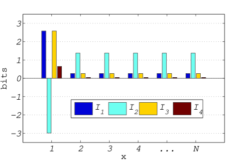
Figure 2: Numerical values of stimulus specific information for different locations $x$. Left, $I_{1,2,3,4}$ considering only firing rate. Place field corresponds to $x=1$. Parameter values: $N=6$, $\sigma=2.5Hz$ and $\overline{r}=20Hz$ for the place field profile.

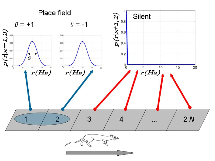
Figure 3: A rat running in linear track (unidirectional). Position in the track is binned, in $2N$ spatial bins. Conditional probability distribution for a place cell: $x_{1}$,$x_{2}$ place field (top, left) for $\theta=1,2$, respectively, and $x_{i\neq 1,2}$ (top, right), outside place field.

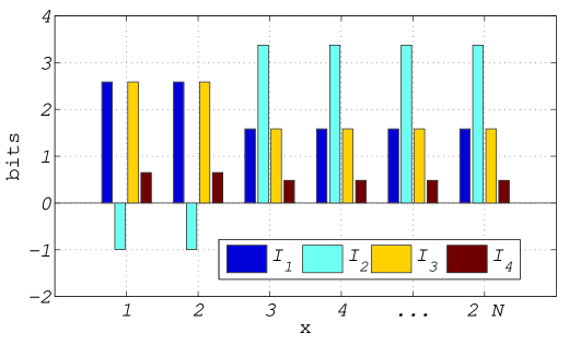
Figure 4: Numerical values of stimulus specific information for different locations $x$. $I_{1,2,3,4}$ considering firing rate and phase-shift (binary values). Place field corresponds to $x=1$ and $x=2$. Parameter values: $N=6$, $\sigma=2.5Hz$ and $\overline{r}=20Hz$ for the place field profile.

To show the different behavior of stimulus specific informations in a more realistic setting, we consider here the example of spatial encoding in hippocampal place cell.

Place cells selectively fire at an elevated rate when the animal is in a particular location of an environment and, in some cases (e.g. linear tracks), moving in one specific direction. For sake of simplicity we do not consider direction here. Place cell firing profile is then characterized by a silent part (when the animal is not in the place field), and an active part corresponding to the place field. Let us consider an ideal experiment in which a rat is moving in a linear track in one direction at constant speed (from left to right in Fig. 1). The set of locations is the stimuli set, that we consider discrete and finite, composed by $N$ elements. We indicate with ${x\in{\cal X}}$ a single position with $p(x)=1/N$. $x_{1}$ corresponds to the place field, and we measure the firing rate of the cell $r$, in each spatial bin $x$. Assuming a gaussian profile inside the place field (see Fig. 1, top-left), and considering the cell completely silent elsewhere (i.e. neglecting fluctuations, Fig. 1, top-right), we are able to compute analytically $I_{1,2,3,4}$ and the mutual information. Results are summarised in Fig. 2. $I_{2}(x_{1})$ may be negative if $\sigma$ is large enough, due to the fact that the uncertainty of the response $H({\cal R}|x)$ could be larger than average uncertainty in the correspondence to the place field. This implies that place-field corresponds to the less informative stimulus according to $I_{2}$ measure. On the contrary, using the other definitions $x_{1}$ is largely the most informative location in agreement with our intuitive notion that the cell codes for the position corresponding to the place field.

To better illustrating the role of additivity rule (Eq. 3), let us consider a simple extension of the previous example, where two different aspects of single cell neural response are considered. In a similar setup, we measure the average firing rate and the phase shift respect to a specific rhythm: the theta oscillations $\Theta$. Indeed, during locomotion hippocampus is characterized by a high-amplitude 4-8 Hz oscillation, called theta rhythm. Theta oscillations play an important role in spatial encoding. Cell spiking shifts gradually to earlier phases of the theta cycle as the animal moves through the cell place field (theta phase precession)[14].

For sake of simplicity, in our toy-example, we take this quantity to assume just two values: $\theta=+$ (say a phase shift of $270^{o}$) and $\theta=-$ (say a phase shift of $90^{o}$), furthermore we associate this feature to non place field location (this is not in general appropriate for real place cells), see Fig. 3. So each cell response is represented by two quantities: firing rate and average phase shift, where the latter is a binary variable. We take finer spatial bins, in this way the place field is covered by two spatial bins. Place cell fires in the place field, corresponding to positions $x_{1}$ and $x_{2}$, with a gaussian profile (as shown in Fig. 3 (top-left)). For $x_{1}$, spike times follow on average theta oscillatory maximum of $\theta=+$ and, vice versa, in $x_{2}$ they come earlier ($\theta=-$). Similarly in the other odd positions $\theta=+$, and $\theta=-$ in the other even positions, where the cell is silent. We neglect fluctuations and we assume that firing rate is zero in these locations.

Overall we have $2N$ different positions. Assuming, as before, all the positions are equally likely $p(x)=\frac{1}{2N}$ and $p(\theta=+)=p(\theta=-)=1/2$, we can analytically estimate mutual information and all the stimulus specific information. Results are summarised in Fig. 4. As in the previous example, place field location corresponds to most informative stimulus according to $I_{1,3,4}$, but less informative for $I_{2}$. Furthermore, in this example, we can test if $r$ and $\theta$ encode different aspects of stimulus $x$ independently or not, checking if: $I(\{{\cal R},{\Theta}\},x)=I({\Theta},x)+I({\cal R},x)$. These terms can be computed analytically using the assumptions above. We find that, using $I_{1,2,3}$ phase and average firing rate encode a single position $x$ independentely. Since averaging these quantities over the stimulus set we have mutual information, independence condition is satisfied for mutual information. On the contrary we have redundant encoding using $I_{4}$. This discrepancy between the behavior of $I_{1,2,3}$ and $I_{4}$ (and mutual information too) is due to the fact that, considering local information, we implicitly correlate the two response features putting together all the locations different from $x_{1}$, so that phase and average firing rate are mixed together in $p(\{{\cal R},{\Theta}\}|\bar{x_{1}})$

Note, to apply the same criterium to test encoding independence for different stimuli features $S_{1},S_{2}$ (e.g. location and direction) only $I_{2}$ may be used.

5 Conclusions

Shannon mutual information is symmetric for stimulus and response set. When we consider stimulus specific information, we lose this symmetry property, resulting in a weaker additivity condition, limited to the response set. So, although none of definitions of stimulus specific information has all the mathematical properties of mutual information, all of them may be used for exploring correlated encoding by multiple response features. In addition, we have shown that different stimulus specific information measures are suitable to answer different questions, and, not surprisingly, they may assume different numerical values in the same context. In conclusion, there is no unique definition, but the right measure should be chosen according to the aspect of neural coding we are interested in studying.

Acknowledgments

We thank A. Arleo and F. Linaker for critical reading of the manuscript.

References

- [1] Shannon, C. E. & Weaver, W., 1949. The mathematical theory of communication. University of Illinois Press.
- [2] Treves, A. & Panzeri, S., 1995. The upward bias in measures of information derived from limited data samples. Neural Comp., 7:399 407.
- [3] Strong, S. P., Koberle, R., de Ruyter van Steveninck, R. R., and Bialek, W., 1998. Entropy and information in neural spike trains, Phys. Rev. Lett., 80(1):197 200.
- [4] Schneidman, E., Bialek, W., & Berry II, M. J., 2003. Synergy, redundancy, and independence in population codes, J Neurosci 23, 11539-11553
- [5] Bezzi, M., Nieus, T., Arleo, A., D’Angelo, E., Coenen, O. J. M., 2004. Information transfer at the mossy fiber-granule cell synapse of the cerebellum, Society for Neuroscience Abstracts 827.5.
- [6] Machens, C. K., Gollisch, T, , Kolesnikova, O., Herz, A. V. M., 2005. Testing the Efficiency of Sensory Coding with Optimal Stimulus Ensembles, Neuron, 47: 447-456
- [7] Fano, R. M., 1961. Transmission of Information; A Statistical Theory of Communications (New York: MIT)
- [8] Rolls, E. T., Treves, A., Tovee, M. J., Panzeri, S., 1997. Information in the neuronal representation of individual stimuli in the primate temporal visual cortex. J. Comput. Neurosci., 4: 309 333
- [9] Lu, T., Wang, X., 2004. Information content of auditory cortical responses to time-varying acoustic stimuli. J. Neurophysiol, 91(1):301-13
- [10] Paz, R., Vaadia, E., 2004. Learning-Induced Improvement in Encoding and Decoding of Specific Movement Directions by Neurons in the Primary Motor Cortex. PLoS Biol, 2(2): e45
- [11] De Weese, M. R., & Meister, M., 1999. How to measure the information gained from one symbol. Network, 10, 325-340.
- [12] Bezzi, M., Samengo, I. , Leutbeg, S., Mizumori, S. J. Y., 2002. Measuring information spatial densities, Neural Computation, 14, 2.
- [13] Butt, D., 2003. How much information is associated with a particular stimulus? Network: Comput. Neural Syst., 14 177-187
- [14] O’Keefe, J., & Recce, M. L. 1993. Phase relationship between hippocampal place units and the EEG theta rhythm. Hippocampus, 3, 317-330
- [15] Harris, K. D., Henze, D. A., Hirase, H., Leinekugel, X., Dragoi, G., Czurko, A., Buzsaki, G., 2002. Spike train dynamics predicts theta-related phase precession in hippocampal pyramidal cells. Nature, 13, 417(6890):738-41.