Optimal Dynamical Range of Excitable Networks at Criticality

Abstract

A recurrent idea in the study of complex systems is that optimal information processing is to be found near bifurcation points or phase transitions. However, this heuristic hypothesis has few (if any) concrete realizations where a standard and biologically relevant quantity is optimized at criticality. Here we give a clear example of such a phenomenon: a network of excitable elements has its sensitivity and dynamic range maximized at the critical point of a non-equilibrium phase transition. Our results are compatible with the essential role of gap junctions in olfactory glomeruli and retinal ganglionar cell output. Synchronization and global oscillations also appear in the network dynamics. We propose that the main functional role of electrical coupling is to provide an enhancement of dynamic range, therefore allowing the coding of information spanning several orders of magnitude. The mechanism could provide a microscopic neural basis for psychophysical laws.

Psychophysics is probably the first experimental area in neuropsychology, having been founded by physiologists (Helmholtz and Weber) and physicists (Fechner, Plateau, Maxwell and Mach) in the middle of the nineteenth century Stevens (1975). Its aim is to study how physical stimuli transduce into psychological sensation, probably the most basic mind-brain problem. How to relate such high-level psychological phenomena to low-level neurophysiology is a task for the twenty-first century brain sciences.

As the intensity of physical stimuli (light, sound, pressure, odorant concentration etc) varies by several orders of magnitude, psychophysical laws must have a large dynamical range. Although this has been extensively verified experimentally at the psychological Stevens (1975) and neural Wachowiak and Cohen (2001); Angioy et al. (2003); Fried et al. (2002) level, little work has been done regarding the mechanism that produces such psychophysical laws Cleland and Linster (1999); Copelli et al. (2002); Copelli and Kinouchi (2005); Copelli et al. (2005). However, two main ideas seem to be consensual: (1) nonlinear transduction must be done at the sensory periphery to prevent early saturation Stevens (1975); and (2) the broad dynamic range is often a collective phenomenon Stevens (1975); Cleland and Linster (1999); Copelli et al. (2002), because single cells usually respond in a linear saturating way with small ranges Reiser and Matthews (2001); Tomaru and Kurahashi (2005).

Two nonlinear transfer functions have been widely used to fit experimental data, both in psychophysics and in neural response: the logarithm function $F(S)=C\log S$ (Weber-Fechner law) and the power law function $F(S)=CS^{m}$ (Stevens Law), where $S$ is the stimulus level, $C$ is a constant and $m$ is the Stevens exponent. Later, other functions have been proposed to fit data with more extended input range, and to account for sensory saturation, in particular the Hill function $F(S)=F_{max}S^{m}/(S^{m}+S_{0}^{m})$ where $F_{max}$ is the saturation response and $S_{0}$ is the input level for half-maximum response. Notice that, because both Hill and Stevens functions have a power law regime, it is natural to denote the exponents by the same parameter $m$.

Some authors have tried to derive such phenomenological laws from the structure of natural signals Chater and Brown (1999). This type of work may furnish an evolutionary motivation for biological organisms to implement or approximate such laws. However, there is no consensual view on this theoretical aspect, and it does not provide a neural basis for implementing the psychophysical laws.

In contrast, our statistical physics approach to neural psychophysics Copelli et al. (2002); Copelli and Kinouchi (2005); Copelli et al. (2005); Furtado and Copelli (2006) shows how Hill-like transfer functions may arise in biological excitable systems: they are not put into the models by hand, nor mathematically derived from a priori reasoning, but appear as a cooperative effect in a network of excitable elements. At differente biological levels, these elements may be interpreted as whole neurons, excitable dendrites, axons, or other subcellular excitable units. We show that a network of excitable elements, each with small dynamic range, presents a collective response with broad dynamic range and high sensitivity. Even more interesting, we find that the dynamic range is maximized if the spontaneous activity of the network corresponds to a critical process. This is compatible with recent findings of critical avalanches in in vitro neural networks Beggs03 ; Haldeman and Beggs (2005) and provides a clearcut example of optimal information processing at criticality Langton (1990); Chialvo (2004); bak . The model also has other dynamical features and permits us to make a testable prediction.

In previous work we have introduced the idea that excitable waves in active media provide a mechanism for strong nonlinear amplification with large dynamic range. This has been shown in simulations with one-dimensional Copelli et al. (2002) and two-dimensional Copelli and Kinouchi (2005) deterministic cellular automaton models, as well as with one-dimensional networks of coupled maps and Hodgkin-Huxley elements Copelli et al. (2005). Analytical results have recently been obtained for the one-dimensional cellular automaton model under the two-site mean-field approximation Furtado and Copelli (2006). In this paper, we study a very different system where the activity propagation is stochastic and the electrical synapses form a random network. This latter case seems to be a more realistic topology for, say, the olfactory intraglomerular network of excitable dendrites coupled by gap junctions Kosaka et al. (2005); Migliore et al. (2005); Christie et al. (2005). We find a whole new phenomenology related to a non-equilibrium phase transition to re-entrant activity present in this model.

In the present model, each excitable element $i=1,\ldots,N$ has $n$ states: $s_{i}=0$ is the resting state, $s_{i}=1$ corresponds to excitation and the remaining $s_{i}=2,\ldots,n-1$ are refractory states. There are two ways for the $i$th element to go from state $s_{i}=0$ to $1$: (1) owing to an external stimulus, modelled here by a Poisson process with rate $r$ (which implies a transition with probability $\lambda=1-\exp(-r\Delta t)$ per time step); (2) with probability $p_{ij}$, owing to a neighbour $j$ being in the excited state in the previous time step. Time is discrete (we assume $\Delta t=1$ ms) and the dynamics, after excitation, is deterministic: if $s_{i}=1$, then in the next time step its state changes to $s_{i}=2$ and so on until the state $s_{i}=n-1$ leads to the $s_{i}=0$ resting state, so the element is a cyclic cellular automaton Marro and Dickman (1999). The Poisson rate $r$ will be assumed to be proportional to the stimulus level $S$ (for example, the odorant concentration in olfactory processing). Notice that each element receives external signals independently, that is, we have a Poisson process for each element (modelling the arrival of axonal inputs from different receptor neurons).

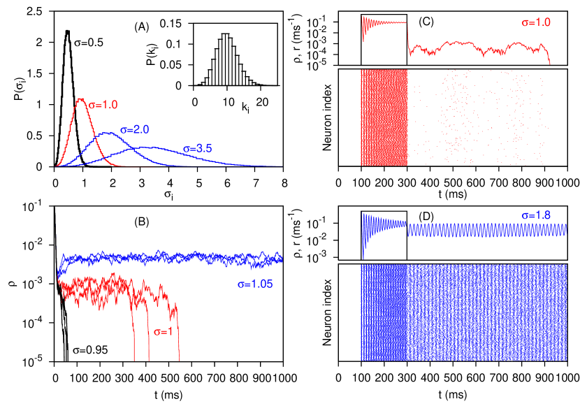
Figure 1: Network characterization and density of active sites. Simulations with $N=10^{5}$ sites, $K=10$ and $n=10$ states. (A) Probability density function of local branching ratio and (inset) connectivity (“degree”) distribution; (B) Instantaneous density of active sites for subcritical (black), critical (red) and supercritical (blue) branching parameters as functions of time (three different runs for each case); (C), (D) Instantaneous density (of all sites; upper panels) and raster plot (of $10^{3}$ randomly chosen sites; lower panels) in response to a square pulse of stimulus ($r=0.5$ ms^-1 for 100 ms $\leq t\leq$ 300 ms, null otherwise) for critical (C) and supercritical (D) branching parameters.

The network with $N$ elements is an Erdős-Rényi undirected random graph, with $NK/2$ links being assigned to randomly chosen pairs of elements. This produces an average connectivity $K$ where each element $i$ $(i=1,\ldots,N)$ is randomly connected to $K_{i}$ neighbours. The distribution $P(K_{i})$ of neighbours is a binomial distribution with average $K$ (see Fig 1A). The probability that an active neighbour $j$ excites element $i$ is given by $p_{ij}$, a random variable with uniform distribution in the interval $[0,p_{max}]$. The weights are symmetrical ($p_{ij}=p_{ji}$) and are kept fixed throughout each simulation (“quenched disorder”). This kind of coupling models electric gap junctions instead of chemical synapses because it is fast and bi-directional. However, symmetry is not a necessary ingredient, because similar results are obtained in asymmetrical networks. Note that we are not assuming that gap junctions have a stochastic dynamics, but only that, because other internal factors and noise are also present, a probabilistic account of the excitation process may be more realistic.

The local branching ratio $\sigma_{j}=\sum_{i}^{K_{j}}p_{ij}$ corresponds to the average number of excitations created in the next time step by the $j$-th element Haldeman and Beggs (2005). The distribution $P(\sigma_{j})$ of local branching ratios (a bell-shaped distribution with average $\sigma=\left<\sigma_{i}\right>$) is shown in Fig. 1A. The average branching ratio $\sigma$ is the relevant control parameter. In the simulations, we set $\sigma$ by choosing $p_{max}=2\sigma/K$ and keeping $\sigma<K/2$.

The network instantaneous activity is the density $\rho_{t}$ of active ($s=1$) sites at a given time $t$. We also define the average activity $F=T^{-1}\sum_{t=1}^{T}\rho_{t}$ where $T$ is a large time window (of the order of $10^{3}$ time steps). Typical $\rho_{t}$ curves in the absence of stimulus ($r=0$) are shown in Fig. 1B. Notwithstanding the large variance of $P(\sigma_{j})$, only supercritical networks (that is, with $\sigma>\sigma_{c}=1$) have self-sustained activity, $F>0$. As expected, critical networks have a larger variance in the distribution of extinction times and present a power law behaviour in the distribution of avalanche sizes with exponent $3/2$ (not shown), in agreement with findings in biological networks Beggs03 .

Two types of oscillations are observed in this system. Under sufficiently strong stimulation, all networks present transient collective oscillations, with frequencies of the order of the inverse refractory period (Fig. 1C). They are a simple consequence of the excitable dynamics and the sudden synchronous activation by stimulus initiation. This transient behaviour is reminiscent of oscillations widely observed in experiments Laurent (2002). Networks with $\sigma>\sigma_{osc}>\sigma_{c}$ also present self-sustained oscillations in the absence of stimulus (Fig. 1D), where $\sigma_{osc}$ is a bifurcation threshold. The frequency depends on the network parameters, but remain in the gamma range $30-60$ Hz. The oscillations are similar to reentrant activity found in spatially extended models of electrically coupled networks Lewis and Rinzel (2001), from which analytical techniques for calculating the frequency could perhaps be borrowed lewis2000 . We remark that the large time window used in the definition of $F$ is only chosen for convenience, as it can be seen from Figs. 1C,D and 200 ms is sufficient to give reliable averages.

As a function of the stimulus intensity $r$, networks have a minimum response $F_{0}$ (= 0 for the subcritical and critical cases) and a maximum response $F_{max}$. We define the dynamic range $\Delta=10\log(r_{0.9}/r_{0.1})$ as the stimulus interval (measured in dB) where variations in $r$ can be robustly coded by variations in $F$, discarding stimuli which are too weak to be distinguished from $F_{0}$ or too close to saturation. The range $[r_{0.1},r_{0.9}]$ is found from its corresponding response interval $[F_{0.1},F_{0.9}]$, where $F_{x}=F_{0}+x(F_{max}-F_{0})$ (see Fig. 2C). This choice of a 10%-90% interval is arbitrary, but is standard in the literature and does not affect our results.

As can be seen in Figs. 2A and 2B, the response curves $F(r)$ of the networks present a strong enhancement of dynamic range compared with the uncoupled case $\sigma=0$. In the subcritical regime, sensitivity is enlarged because weak stimuli are amplified due to activity propagation among neighbours. As a result, the dynamic range $\Delta(\sigma)$ increases monotonically with $\sigma$. In the supercritical regime, the spontaneous activity $F_{0}$ masks the presence of weak stimuli, therefore $\Delta(\sigma)$ decreases. The optimal regime occurs precisely at the critical point (see Fig. 2D). This is a new and important result, because it is perhaps the first clear example of signal processing optimization at a phase transition, making use of a standard and easily measurable performance index.

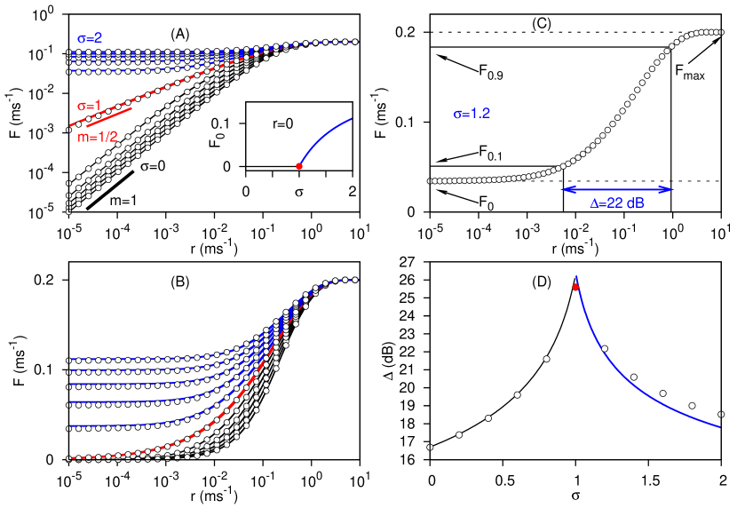
Figure 2: Response curves and dynamic range. Points represent simulation results with $N=10^{5}$ sites, $K=10$, $n=5$ states and $T=10^{3}$ ms, whereas lines correspond to the mean-field model described in the text. (A) Response curves (mean firing rate vs. stimulus rate) from $\sigma=0$ to $\sigma=2$ (in intervals of 0.2). Line segments are power laws $F\propto r^{m}$ with $m=1$ (subcritical) and $m=1/2$ (critical). Inset: spontaneous activity $F_{0}$ vs. branching ratio $\sigma$. (B) The same as in (A), but with a linear vertical scale. (C) Response curve for $\sigma=1.2$ and relevant parameters for calculating the dynamic range $\Delta$. (D) Dynamic range vs. branching ratio is optimized at the critical point $\sigma=1$.

The curves $F(r)$ could be fitted by a Hill function, but are not exactly Hill. The theoretical curves in Fig. 2 are obtained from a simple mean-field calculation (see below) that provides a very good fit to the simulation data without free parameters, and correctly predicts the exponents governing the low-stimulus response $F\propto r^{m}$. An important point is that the Stevens-Hill exponent $m$ changes from $m=1$ in the subcritical regime to $m=0.5$ at criticality. If we assume that biological networks work in the optimal regime, the critical value $m=0.5$ suggests how exponents less than one could emerge in psychophysics Stevens (1975) and neural responses Wachowiak and Cohen (2001); Fried et al. (2002). We note that apparent exponents between 0.5 and 1.0 are observed Furtado and Copelli (2006) if finite size effects are present, that is, if $N$ is small.

In the simple mean-field approximation, we take $K_{i}=K$ and $p_{ij}$ as the average value $\sigma/K$. The probability $p_{t}$ that an inactive site at time $t$ will be activated in the next time step by at least one of its $K$ neighbours (a fraction $F_{t}$ of which is currently active) is simply $p_{t}=1-(1-\sigma F_{t}/K)^{K}$. This leads to the following mean-field map:

$$F_{t+1}=P_{t}(0)\lambda+P_{t}(0)(1-\lambda)p_{t}\;,$$ (1)

where

$$P_{t}(0)=1-(n-1)F_{t}$$ (2)

is the approximate probability of finding a site in the resting state and $\lambda(r)=1-\exp(-r\Delta t)$. The first term on the right-hand side of equation 1 corresponds to activation due to external input, and the second term corresponds to activation due to neighbour propagation. In the stationary regime, the response function $F(r)$ is given by the solution of

$$F=\left(1-(n-1)F\right)\left[1-(1-\sigma F/K)^{K}\left(1-\lambda(r)\right)\right]\;.$$ (3)

Note that equation 2 is only exact in the stationary state, but the resulting map is consistent because the result of its iterations coincides with the solution of equation 3 (in particular, $F\leq 1/n$, so that $P(0)\geq 0$).

As is usual in the statistical physics of phase transitions Marro and Dickman (1999), we analyse two limits: the critical behavior without an external field and the effect of a vanishing field at the critical point. In the absence of external stimulus ($\lambda=0$), in the limit $\sigma\to\sigma_{c}=1$ ($F\to 0$), the order parameter behaviour is $F(\sigma)\simeq(\sigma-1)/C$ where $C=(n-1)+(K-1)/2K$, which gives, from the definition $F(\sigma)\propto(\sigma-\sigma_{c})^{\beta}$, a critical exponent $\beta=1$. On the other hand, at the critical point $\sigma=\sigma=1$ we have $F(r)\approx\sqrt{r/C}$ which gives the Stevens exponent $m=1/2$. Notice that the rate $r$ plays the role of an external field $h$ and, from the usual statistical-physics definition Marro and Dickman (1999) $F\propto h^{1/\delta_{h}}$ we get the critical exponent $\delta_{h}=2$. As expected, these are the classical mean-field exponents for branching processes, which seem to be valid for our model even with the presence of quenched disorder. An important conceptual point is that the Stevens-Hill exponent is indeed found to be indeed a statistical-physics critical exponent $m=1/\delta_{h}$.

Optimization of dynamic range at criticality is very robust; the shape of the plot in Fig. 2D does not depend on parameters such as the average number of neighbours $K$ or refractory period $n$. The random-network case seems to be a lower bound for the dynamic-range enhancement. In future works, we will report that $\Delta(\sigma)$ is even more enhanced in low-dimensional networks, and presents non-rational Stevens exponents. Perhaps a better compromise between larger dynamic range and biological realism would be a small-world or scale-free network.

As an example of the robustness of the results, if we put Hodgkin-Huxley elements with coupling with values $p_{ij}=0$ or 1, which would correspond to a deterministic case with the presence of absence of bonds, we obtain a $\Delta(p)$ curve, where $p$ is the probability that a bond exists between the elements. This $\Delta(p)$ curve is very similar to the $\Delta(\sigma)$ curve of the present model, that is, $\Delta(p)$ has a strong peak at the percolation phase transition $p=p_{c}$ (to be reported elsewhere). However, the present model has the virtue of enabling analytical results that provide a benchmark for the performance of networks with other topologies.

Now we discuss the possible relevance of our results to biological sensory processing. Recent findings show that projection cells in sensory systems are coupled via dendro-dendritic electrical synapses, for example $\alpha$-ganglionar cells in the retina Schubert et al. (2005); Hidaka et al. (2005) and mitral cells in the olfactory bulb Kosaka et al. (2005); Migliore et al. (2005); Christie et al. (2005). In most of these findings the electrical coupling is mediated by connexins, but pannexins could also be present, and could even be more important than connexins for providing electrical coupling between excitatory cells Vogt et al. (2005). However, the functional role of this electrical coupling is largely unknown. We propose that the electrically coupled dendritic trees in these systems form an excitable network (where each element of our model represents an excitable dendritic patch). Our results are consistent with the reduction in sensitivity, dynamical range and synchronization recently observed in retinal ganglion cell response of connexin-36 knockout mice Deans et al. (2002).

In the case of olfactory system, we identify the excitable random network with the dendro-dendritic network in the glomeruli Kosaka et al. (2005), and each element is interpreted as an active dendritic compartment containing ion channels. It is known that relevant electrical coupling between mitral cells is done at the glomerular level Migliore et al. (2005); Christie et al. (2005) because only cells that have their apical dendrite tufts in the same glomerulus show synchronized activity. In connexin-36 knockout mice, the synchronized activity of mitral cells is absent.

Our hypothesis could be tested in the following way. The dynamic range of glomeruli is of the order of 30 dB as measured recently Wachowiak and Cohen (2001); Fried et al. (2002) (in contrast to 10 dB of single olfactory receptor neurons). We predict that in connexin-36 knockout mice, this dynamic range shall be strongly reduced. Of course, for a decisive test, we need to examine if other electrical synapses based on connexin-45 Zhang and Restrepo (2002) and pannexins Vogt et al. (2005) are irrelevant in olfactory glomeruli.

The text-book account of large dynamic range in intensity coding is the recruitment model or its variants Cleland and Linster (1999) where different elements, with diverse activation thresholds, are sequentially recruited. Our mechanism is not incompatible with this scenario, and we expect that threshold variability in our model enlarges the dynamic range even more. However, we must remember that recruitment is a linear mechanism where, to explain each order of magnitude in dynamic range, we must postulate a corresponding order of magnitude in activation thresholds, which is not a plausible assumption Cleland and Linster (1999).

We may ask how the network could self-organize to the critical point $\sigma_{c}=1$. It is not hard to conceive that homeostatic mechanisms, acting on the number and conductance of gap junctions, could tune the system. It is well known that extensive pruning of gap junctions occurs during development and maturation. This could represent the initial self-organization process towards criticality. Spontaneous activity in the absence of input furnishes a signature of supercriticality that could be used as a feedback signal to control the system.

This self-tuning criticality has recently been proposed in a model of sound nonlinear amplification by Hopf oscillators in the cochlea Camalet00 . In the cochlear model, it is assumed that each oscillator is poised at its Hopf bifurcation point, producing enhanced sensitivity and enlarged dynamic range. The principal difference from our mechanism is that it is a model for individual cells, that is, it is not based on a collective phenomenon. This implies that the dynamic-range exponent must be classical (rational). In our case, the rational exponent $m=1/2$ is a particularity of the random network, and, similarly to other statistical-mechanics models, more-structured network topologies may have non-classical exponents.

Although in this work we restricted our attention to sensory processing, we note that the dynamic range of more central networks could also be improved by the same mechanism. Similarly to excitatory networks, inhibitory networks must also work robustly in the presence of large variations in input. So, the presence of electrical synapses in cortical inhibitory networks Sohl et al. (2005) could reflect the same principle.

The mechanism for amplified nonlinear response due to wave creation and annihilation is a basic property of excitable media. We found in this work that, if active media are tuned at the critical point of activity propagation, the response is optimized. We proposed that this principle is present in electrically coupled excitable dendritic networks in projection neurons of sensory systems and is a generative mechanism for psychophysical laws. This computational principle based in critical activity could also be present in other brain regions and could be implemented in artificial sensors by using excitable media as detectors.