Protein folding dynamics via quantification of kinematic energy landscape

Abstract

We study folding dynamics of protein-like sequences on square lattice using physical move set that exhausts all possible conformational changes. By analytically solving the master equation, we follow the time-dependent probabilities of occupancy of all 802,075 conformations of 16-mers over 7-orders of time span. We find that (i) folding rates of these protein-like sequences of same length can differ by 4-orders of magnitude, (ii) folding rates of sequences of the same conformation can differ by a factor of 190, and (iii) parameters of the native structures, designability, and thermodynamic properties are weak predictors of the folding rates, rather, basin analysis of the kinematic energy landscape defined by the moves can provide excellent account of the observed folding rates.

The dynamics of protein folding has been studied extensively PlaxcoBaker-JMB ; rateModel . A remarkable observation is that protein folding rates are well correlated with their native structural properties PlaxcoBaker-JMB . A native centric view postulates that protein folding rates are largely determined by the topology of its native structure GillespiePlaxco . Theoretical models using Gō potential where only native contacts contribute energetically are very successful in reproducing observed folding rates rateModel ; WeiklDill .

However, the extent to which native structure determines folding rate remains unclear. By the native-centric view, different sequences for the same protein structural fold would all have very similar folding rates, as they share essentially the same native structure topology. However, this is not consistent with experimental results. As the folding rates of simple single-domain proteins differ by 6 orders of magnitude GillespiePlaxco , folding rates may be very heterogeneous. A recent experimental study showed that a designed artificial protein with no homologous sequence in nature that adopts the same structure as a natural protein can fold 4,000 times faster Scalley-Kim-Baker-04 . A distinct possibility is that the empirical correlation between properties of native protein structures and folding rates may arise from inadequate sampling in the sequence space due to accumulated biased natural selection and limited genetic drift, rather than from intrinsic physical properties of proteins.

In this letter, we use two-dimensional hydrophobic and polar (HP) lattice model ChanDill94 to study the relationship of folding rates, native structure topology, thermodynamic properties, and effects of sequence variation. We model the physical movement of protein chains. Real protein cannot immediately jump from one conformation to another arbitrary conformation. Two conformations of the same energy may be well separated kinetically. We regard protein movement as a sequence of successive conformational changes, each represented by a physically realizable primitive move. The physical move set we developed exhausts all possible conformational changes for a structure. We use master equation to study the folding dynamics of foldable sequences of length 16. While master equation provides an exact solution ChanDill94 ; Cieplak98-PRL , in the past it was necessary to cluster conformations of larger systems into macrostates to reduce the size of the transition matrix OzkanBaharDill-NSB , therefore making the use of physical moves infeasible. Here we directly solve the eigenvalue problem of the 802,075 $\times$ 802,075 transition matrix and develop a method to monitor the time-dependent probability of occupancy of all conformations simultaneously from the first kinetic move until reaching half-equilibrium concentration over 7-orders of time scale.

Our results show that the properties of native structure, designability, and thermodynamic properties are inadequate to explain protein folding dynamics in our model systems. We found that protein-like sequences can fold into the same native structure with folding rates differ as much as 190 times and sequences of the same length and energy gap can differ by 4-orders of magnitude in folding rate. Instead of thermodynamic properties, we show that properties of the move-connected energy landscape defined by the connection graph of physical moves can provide excellent account for observed folding rates.

Model. We use the following energy model for different types of nonbonded HP contacts: $E_{HH}=1$, $E_{HP}=0$, and $E_{PP}=0$. By evaluating the energy level of all $2^{16}$ sequences of 16-mers on all enumerated $|\Omega|=802,075$ conformations, we have identified 26 sequences that all fold into the same ground state conformation (Fig. 1). This set of sequences forms the largest protein family, where each sequence adopts the same conformation, and all are connected by (a series of) point mutations. Altogether, there are 1,539 foldable sequences with unique ground state conformations. There are 456 conformations that are the unique ground state for 1 or more foldable sequences.

We develop a set of physically possible primitive moves (Fig. 1c). They are generalizations of corner move, crankshaft move, and pivot move. We exhaust all possible occurrence of such moves for every conformation. We verified that this move set is ergodic, i.e., all conformations are connected to each other by a series of primitive moves. With this move set, the simple energy scheme of the HP model leads to a complex energy landscapes, with numerous local minima for a foldable sequence.

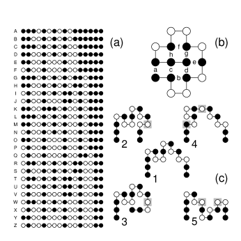
Figure 1: Protein-like sequences and the set of primitive moves. The largest protein family contains (a) 26 sequences that all fold into (b) the same structure. Here filled circles are H residues. (c) The move set includes: among (1, 2, and 3), single point moves rotate around a single point; between (1 and 4), generalized corner moves reflect around a diagonal axis connecting any two residues; between (1 and 5), generalized crankshaft moves reflect around a horizontal or vertical axis. Points of rotation are on gray background. For a given conformation, we exhaustively search all possible position for point moves, all possible pairs of positions for possible generalized corner moves and generalized crankshaft moves.

We use Metropolis-type of dynamics to assign the transition rate $r_{ij}$ from conformation $i$ to a neighbor conformation $j$ connected by a move: $r_{ij}=1$ if $E(j)\leq E(i)$; $r_{ij}=e^{-[E(j)-E(i)]/T}$ if $E(j)>E(i)$; and $r_{ij}=-\sum_{i\neq k}r_{ik}$, if $j=i$. For non-neighbors, $r_{ij}=0$. We assume the effects of viscosity and friction are negligible.

We follow Cieplak98-PRL ; OzkanBaharDill-NSB and use a master equation to study protein folding dynamics. Let $p_{i}(t)$ be the probability that the HP molecule takes the $i$-th conformation at the time $t$, then $dp_{i}(t)/dt=\sum_{i\neq j}[r_{ji}p_{j}(t)-r_{ij}p_{i}(t)]$. Written in vector form, we have: $d{\mbox{\boldmath$p$}}(t)/dt={\mbox{\boldmath$R$}}{\mbox{\boldmath$p$}}(t),$ where $R$ is the rate matrix whose entries are defined by the above expression. We choose temperature $T=0.2$ in unit of $\Delta E_{HH}/k_{B}$, which is below the folding temperature $T_{f}$ when 50% of molecules take the native conformation. $T_{f}$ varies from $\sim 0.2$ to $\sim 0.5$ for different sequences.

A general solution of the master equation can be written as ${\mbox{\boldmath$p$}}(t)=\sum_{i}C_{i}{\mbox{\boldmath$n$}}_{i}e^{-\lambda_{i}t}$ with $C_{i}={\mbox{\boldmath$v$}}_{i}^{T}{\mbox{\boldmath$p$}}(0)$, where $\lambda_{i}$ is the $i$-the eigenvalue of the rate matrix $R$, ${\mbox{\boldmath$n$}}_{i}$ the corresponding right eigenvector, ${\mbox{\boldmath$v$}}_{i}$ the left eigenvector, and ${\mbox{\boldmath$p$}}(0)$ the initial vector of distribution of conformations. In this study, we use the high temperature condition and assign ${\mbox{\boldmath$p$}}(0)={\mathbb{1}}/|\Omega|$. Two eigenvalues are of particular interest: $\lambda_{0}=0$ corresponds to the equilibrium Boltzmann distribution, and the smallest none-zero eigenvalue $\lambda_{1}$ determines the slowest mode of relaxation. Following OzkanBaharDill-NSB , we take $\lambda_{1}$ as the folding rate $k_{f}$ of the protein. Although the full computation of all eigenvalues and eigenvectors for a $802,075\times 802,075$ matrix $M$ is infeasible, $\lambda_{1}$ and the corresponding eigenvectors ${\mbox{\boldmath$n$}}_{1}$ and ${\mbox{\boldmath$v$}}_{1}$ can be computed by an Arnoldi method.

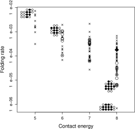
Figure 2: The correlation of $\log k_{f}$ and ground state contact energy. A circle represents one of the 26 sequences shown in Fig. 1, a cross represents one of the 79 singleton sequences, and the diamond represents the Gō model. Native conformations for a few sequences are also shown.

Thermodynamics and folding rates. Several thermodynamic properties have been proposed to be determinants of protein folding rates. We found that protein stability as measured by the total contact energy are correlated with $\log k_{f}$ ($R^{2}=0.71$), i.e., more stable proteins fold slower in general (Fig. 2). Because stable proteins have lower ground state energy, some local minima will also have relatively deep energy traps. As a result, more stable proteins will have slower folding rates because they can be trapped in such local minima. However, the folding rates of sequences of the same ground state energy can still differ as much as $10^{4}$. The heterogeneity of folding rate was already noted in an earlier study using macrostate approximation ChanDill94 . Here we found that even sequences that fold into the same conformation shown in Fig. 1a demonstrate a wide range of rates, from $1.1\times 10^{-3}$ to $5.8\times 10^{-6}$, which is much larger than the difference between the average folding rates for sequences of different native state energies. Protein stability therefore provide some but not the main explanation of the heterogeneity of folding rates.

Energy gap between ground state and excited state was thought to be the necessary and sufficient determinant of folding rate Sali94_Nature . For all 1,456 protein-like sequences of $N=16$, the energy gap between the lowest state and the next state is $\Delta E=1$. The diversity in folding rate $k_{f}$ shown in Fig. 2 clearly indicates that energy gap is not a determining factor for the folding rate. The correlation $R^{2}$ between $\log k_{f}$ and energy gap normalized by standard deviation is 0.01.

Another thermodynamic property thought to be an important determinant of folding rates is the collapse cooperativity $\sigma=1-T_{f}/T_{\theta}$ KlimovThirumalai95-PRL , where $T_{f}$ is as defined earlier, and $T_{\theta}$ the temperature when heat capacity $C(T)$ reaches its maximum. Fig. 3 shows that for the 26 sequences that fold to the same native structure in Fig. 1b, there is a weak correlation ($R^{2}=0.38$) between collapse cooperativity and $\log k_{f}$. Large variance in observed folding rates exist for sequences of similar collapse cooperativity.

Figure 3: Examples of the correlation of folding rate $k_{f}$ with thermodynamic properties and kinetic landscape properties. (a) $k_{f}$ and collapse cooperativity $\sigma$ have weak correlation ($R^{2}=0.38$). (b) $k_{f}$ has excellent correlation with the number of local minima ($R^{2}=0.85$), a property of the kinetic landscape. The diamond represents the Gō model.

The number of sequences that take a specific conformation as the unique ground state is thought to be correlated with overall protein stability and folding rates Melin . We calculated in addition $k_{f}$ for a group of 79 singleton sequences with no sequence homologs that fold to the same native conformations. The distribution of $k_{f}$s for the singleton sequences and the 26 sequences shown in Fig. 2 demonstrate similarly large variation. For our model, designability is not an important determinant of the folding rates.

The Inverse Participation Ratio $I$ is commonly used to characterize the localization of eigenvectors. It is defined as $I=\sum_{k}v_{k}^{2}$, where $v_{k}$ is the $k$-th coefficient of the normalized eigenvector. The correlation between $I$ for the equlibrium eigenvector and the folding rate for the 26 sequences is rather poor ($R^{2}=2\times 10^{-3}$).

Kinematic determinants of folding landscape. Protein folding kinetics are intrinsically determined by physical movement of molecules. Weak correlations of the folding rate with thermodynamic properties are not surprising. Thermodynamic properties of a sequence can be calculated if its complete set of conformations are enumerated. Such properties are not affected by the kinetic connections between conformations. A smooth energy landscape ensuring fast folding can be easily permuted into a rugged landscape by assuming different transition rules between conformations. Both will have the same thermodynamic properties, but the resulting folding rates for the same sequence will be very different. The energy landscape of folding is dictated by the connection graph of states defined by the move set. Characterizing such kinematic energy landscape is therefore essential for studying protein folding dynamics.

Although the energy landscape contains 802,075 conformations, each is connected by the move set to only a limited number ($\sim$ 30) of conformations. We can identify states that are local minima, i.e., all states connected to which by moves have higher energy. A simple characterization of the kinematic energy landscape is then the number count $n_{\min}$ of the local minima. Fig. 3b shows that an excellent correlation of $\log k_{f}$ and $n_{\min}$ ($R^{2}=0.85$) can be found for the 26 HP sequences that fold into the same conformation.

Our conclusions are not sensitive to temperature $T$. When $T$ is raised from $0.20$ to $0.21$ (equivalent to raising $T$ from $300K$ to $315K$), we found that the folding rate $k_{f}$ of the 26 sequences all increases. Although $k_{f}$ for slow folder increases more (by a factor of 2.0 versus a factor of $1.4$ for fast folders), $k_{f}$ at $T=0.21$ is well-correlated with $k_{f}$ at $T=0.20$. The correlation coefficients of $\log k_{f}$ with the number of local minima, collapse cooperativity (Fig. 3), and other thermodynamic parameters are essentially unchanged.

Time evolution and basin analysis. Monitoring the exact time evolution of all conformations simultaneously until reaching equilibrium during folding is a challenging task. Mathematically, the model of master equation is equivalent to a Markov process, where the population vector of conformations at time $t+k\Delta t$ is given by ${\mbox{\boldmath$p$}}(t+k\Delta t)={\mbox{\boldmath$M$}}^{k}{\mbox{\boldmath$p$}}(t)$, where ${\mbox{\boldmath$M$}}={\mbox{\boldmath$I$}}+{\mbox{\boldmath$R$}}\cdot\Delta t$, $I$ being the identity matrix. However, the $k$-time step Markov matrix ${\mbox{\boldmath$M$}}^{k}$ rapidly becomes a dense matrix, and following the time evolution of folding by a straightforward matrix multiplication of ${\cal O}(|\Omega|^{3}\log k)$ steps becomes impossible for a large matrix of size $|\Omega|=802,075$ and $k=10^{6}-10^{10}$. The analytical solution of ${\mbox{\boldmath$p$}}(t)=\sum_{i}C_{i}{\mbox{\boldmath$n$}}_{i}e^{-\lambda_{i}t}$ through diagonalization is also impractical, as it is only possible to calculate a few eigenvectors and eigenvalues for a large matrix.

We seek an accurate solution without the approximation of macrostates. Taking advantage of the sparsity of the rate matrix $R$, we follow the approach of Sidje Sidje-expokit and use the analytical solution of matrix exponential: ${\mbox{\boldmath$p$}}(t)=e^{{\mbox{\boldmath$R$}}t}{\mbox{\boldmath$p$}}(0),$ where $e^{{\mbox{\boldmath$R$}}t}$ is defined by the Taylor expansion $e^{{\mbox{\boldmath$R$}}t}={\mbox{\boldmath$I$}}+t{\mbox{\boldmath$R$}}+\frac{t^{2}}{2}{\mbox{\boldmath$R$}}^{2}+\cdots+\frac{t^{k}}{k!}{\mbox{\boldmath$R$}}^{k}+\cdots$. This expansion itself is impractical, as it also involves large matrix product of increasing density. Plus, the entries in the matrix terms may have alternating signs and hence cause numerical instability. A better approach is to expand $e^{{\mbox{\boldmath$R$}}t}{\mbox{\boldmath$p$}}(0)$ in the Krylov subspace ${\mathcal{K}}_{m}$ defined as:

$${\mathcal{K}}_{m}({\mbox{\boldmath$R$}}t,{\mbox{\boldmath$p$}}(0))\equiv\mbox{Span}\{{\mbox{\boldmath$p$}}(0),\cdots,({\mbox{\boldmath$R$}}t)^{m-1}{\mbox{\boldmath$p$}}(0)\}.$$ (1)

Denoting $||\cdot||_{2}$ as the 2-norm of a vector or matrix, our approximation then becomes ${\mbox{\boldmath$p$}}(t)\approx||{\mbox{\boldmath$p$}}(0)||_{2}{\mbox{\boldmath$V$}}_{m+1}e^{t\overline{{\mbox{\boldmath$H$}}}_{m+1}}{\mbox{\boldmath$e$}}_{1}$, where ${\mbox{\boldmath$e$}}_{1}$ is the first unit basis vector, ${\mbox{\boldmath$V$}}_{m+1}$ is a $(m+1)\times(m+1)$ matrix formed by the orthonormal basis of the Krylov subspace, and $\overline{{\mbox{\boldmath$H$}}}_{m+1}$ the upper Heisenberg matrix, both computed from an Arnoldi algorithm. The error can be bounded by ${\cal O}(e^{m-t||{\mbox{\boldmath$R$}}||_{2}}(t||{\mbox{\boldmath$R$}}||_{2}/m)^{m})$. We now only need to compute explicitly $e^{\overline{{\mbox{\boldmath$H$}}}_{m+1}t}$. Because $m$ is much smaller than 802,075, this is a simpler problem. A special form of the Padé rational of polynomials instead of Taylor expansion is used for this Sidje-expokit : $e^{t\overline{{\mbox{\boldmath$H$}}}_{m+1}}\approx N_{pp}(t\overline{{\mbox{\boldmath$H$}}}_{m+1})/N_{pp}(-t\overline{{\mbox{\boldmath$H$}}}_{m+1})$, where $N_{pp}(t\overline{{\mbox{\boldmath$H$}}}_{m+1})=\sum_{k=0}^{p}c_{k}(t\overline{{\mbox{\boldmath$H$}}}_{m+1})^{k}$ and $c_{k}=c_{k-1}\cdot\frac{p+1-k}{(2p+1-k)k}$. In our calculation, we select $m=30$.

Figure 4: The time evolution of the native state and several local minima states. The probability of occupation of native state conformation (top) increases monotonically through a time span of $10^{-2}-10^{5}$, but local minima conformations go through transiently accumulating intermediate states.

Fig. 4 shows an example of an HP sequence (sequence C in Fig. 1a) and the time evolution of its native conformation and several local minima conformations. The time evolution of the native conformation shows an initial fast phase upto $t\sim 50$ time units. In principle, the local minima conformations can follow different kinetic processes: Some could be transiently accumulating, and others either monotopically accumulating or monotopically decreasing. Based on the computed trajectories of time evolution, we find that the dynamic behavior of local minima conformations can be predicted from basin analysis of the move-connected energy landscape. We define the size of the basin associated with each local minimum state $i$ computationally by artificially making every local minimum an absorption state, i.e., a sink of infinite depth, such that once reached, no molecule can escape. This is achieved by assigning $r_{ij}=0$ and $r_{ii}=1$ for each local minimum state $i$ ChangCieplak . $p^{\prime}_{i}(t=\infty)$ therefore reflects the size of the basin of the $i$-th local minimum. We define the accumulation ratio as $\varrho=\frac{p^{\prime}_{i}(\infty)}{e^{-E_{i}/T}/\sum_{j}e^{-E_{j}/T}}.$ If $\varrho>1$, state $i$ is most likely a transient accumulating state, i.e., the other conformations in its basin first rapidly flow to state $i$ before transiting to conformations outside the basin. If $\varrho<1$, depending on its initial probability of occupancy and the final Boltzmann factor, state $i$ may be either a monotonically decaying or accumulating state. We find that among the 493 local minima states for this sequence, all except 3 are transiently accumulating, indicating they are responsible for forming transient state ensemble of various time scale.

To understand whether the formation of certain native contacts facilitate folding, we examine the time evolution of each of the 8 native contacts ($a$–$h$) in Fig. 1(b) for the 26 sequences. We found that fast folders have larger amount native contact $d$ ($R^{2}=0.74-0.81$ with $\log k_{f}$), and contact $c$ at the transient time of$50-100$ (Fig. 4), indicating that these contacts are critical for folding by restricting favorably the conforamtional search space. The formation of other native contacts seem not to be directly related to folding rates.

To conclude, we studied protein folding dynamics using a model based on detailed physical moves and exact solution of the master equation. We found that folding rates vary enormously for sequences of the same length, energy, energy gap, and even of the same ground state conformation. In contrast to the thermodynamic parameters which are weak predictors of folding rates, properties of the kinematic landscape defined by the physical moves provide excellent correlation with folding rates. With the computation of time evolution of individual conformation from the first move to half-time of equilibrium, we show that many transiently accumulating intermediate states can be identified by basin analysis.

^∗ Corresponding author. Email: jliang@uic.edu

References

- (1) K.W. Plaxco, K.T. Simons, and D. Baker, J. Mol. Biol. 227, 985 (1998).
- (2) O.V. Galzitskaya and A.V. Finkelstein, Proc. Natl. Acad. Sci. USA 96, 11299 (1999). V. Munoz and W.A. Eaton, Proc. Natl. Acad. Sci. USA 96, 11311 (1999). E. Alm and D. Baker, Proc. Natl. Acad. Sci. USA 96, 11305 (1999).
- (3) B. Gillespie and K.W. Plaxco, Annu. Rev. Biochem. 73, 837 (2004).
- (4) T.R. Weikl and K.A. Dill, J. Mol. Biol. 329, 585 (2003).
- (5) M. Scalley-Kim and D. Baker, J. Mol. Biol. 338, 573 (2004).
- (6) H.S. Chan and K.A. Dill, J. Chem. Phys. 100(12), 9238 (1994).
- (7) M. Cieplak et al., Phys. Rev. Lett. 80, 3654 (1998).
- (8) S.B. Ozkan, K.A. Dill, and I. Bahar, Protein Sci. 11, 1958 (2002).
- (9) A. Šali, E.I. Shakhnovich, and M. Karplus, Nature 369, 248 (1994).
- (10) D.K. Klimov and D. Thirumalai, Phys. Rev. Lett. 76, 4070 (1995).
- (11) R. Melin et al., J. Chem. Phys. 110, 1252 (1999).
- (12) R.B. Sidje, ACM Trans. Math. Softw. 24(1), 130 (1998).
- (13) I. Chang et al., Protein Sci. 13, 2446 (2004).