Force Modulating Dynamic Disorder: Physical Theory of Catch-slip bond Transitions in Receptor-Ligand Forced Dissociation Experiments

Abstract

Recently experiments showed that some adhesive receptor-ligand complexes increase their lifetimes when they are stretched by mechanical force, while the force increase beyond some thresholds their lifetimes decrease. Several specific chemical kinetic models have been developed to explain the intriguing transitions from the “catch-bonds” to the “slip-bonds”. In this work we suggest that the counterintuitive forced dissociation of the complexes is a typical rate process with dynamic disorder. An uniform one-dimension force modulating Agmon-Hopfield model is used to quantitatively describe the transitions observed in the single bond P-selctin glycoprotein ligand 1(PSGL-1)$-$P-selectin forced dissociation experiments, which were respectively carried out on the constant force [Marshall, et al., (2003) Nature 423, 190-193] and the force steady- or jump-ramp [Evans et al., (2004) Proc. Natl. Acad. Sci. USA 98, 11281-11286] modes. Our calculation shows that the novel catch-slip bond transition arises from a competition of the two components of external applied force along the dissociation reaction coordinate and the complex conformational coordinate: the former accelerates the dissociation by lowering the height of the energy barrier between the bound and free states (slip), while the later stabilizes the complex by dragging the system to the higher barrier height (catch).

Adhesive receptor-ligand complexes with unique kinetic and mechanical properties paly key roles in cell aggregation, adhesion and other life’s functions in cells. A well studied example is the receptors in selectin family which comprises E-, L- and P-selectin interacting and forming “bonds” with their glycoprotein ligands. These bonds are primarily responsible for the tethering and rolling of leukocytes on inflamed endothelium under shear stress McEver ; Konstantopoulos98 . In particular, in the past two years great experimental efforts Marshall ; Evans2004 ; Sarangapani ; Yago ; Marshall05 have been devoted to study the surprising kinetic and mechanical behaviors of the bonds between L- and P-selectin and P-selectin glycoprotein ligand 1 (PSGL-1) at the single molecule level: the lifetimes of these bonds first increase with initial application of small force, which are termed “catch” bonds, and subsequently decrease, which are termed “slip” bonds when the force increases beyond some thresholds. The most important biological meaning of this discovery is that the catch-slip transitions of the PSGL-1$-$L- and $-$P-selectin bonds may provide a direct experimental evidence at the single-molecule level to account for the shear threshold effect Finger ; Lawrence , in which the number of rolling leukocytes first increases and then decreases while monotonically increasing shear stress.

On the theoretical side, it is a challenge to give a reasonable physical theory or model to explain the counterintuitive bond transitions. Bell Bell firstly suggested that the force induced dissociation rate of adhesive receptor-ligand complex could be described by,

$$k_{\rm off}(f)=k^{0}_{\rm off}\exp[f\xi^{{\ddagger}}/k_{\rm B}T],$$ (1)

where $k^{0}_{\rm off}$ is the intrinsic dissociation rate constant in the absence of force, $\xi^{{\ddagger}}$ is the distance from the bound state to the energy barrier, $f$ is a projection of external applied force along the dissociation coordinate, $k_{\rm B}$ the Boltzmann’s constant, and $T$ is absolute temperature. The validity of the model has been demonstrated in experiments Alon ; Chen . Although later at least four models have been put forward to explain and understand various receptor-ligand forced dissociation experiments Dembo ; Dembo94 ; Evans97 , they cannot predict catch bonds because force in these models only lowers height of the energy barrier while shortening lifetimes of the bonds. An exception is the Hookean spring model proposed by Dembo many years ago Dembo ; Dembo94 , in which a catch bond was raised in mathematics. Compared to the exponential decay of the lifetimes of slip-bonds with respect to force in experiments Chen , the model claimed that the lifetimes decrease exponentially with the square of force Dembo . In addition, the Hookean spring model cannot account for the catch-slip bond transitions in self-consistent term. Prompted by the intriguing experimental observations, three chemical kinetic models have been developed. Evans et al. presented a two pathways, two bound states model with rapid equilibrium assumption between the two states. They suggested that the catch-slip bond transitions take place due to applied force switching the pathways from the one with slower dissociation rate to the fast one Evans2004 . Although this insightful viewpoint well described force jump-ramp experiments, there are two apparent flaws in physics. First if the forced dissociation experiments were performed at very low temperatures or higher solvent viscosities, force would be independent of the bond dissociations since the force in the two pathways and two bound states model only acts on the inner bound states, while these states would be “frozen” under this circumstances. The other is that force does not accelerate the dissociation processes further when the force is sufficiently large for the fast dissociation rate is a constant. The next model given by Barsegov and Thirumalai Barsegov with same kinetic scheme seems to improve the two flaws in which the dissociation rates of the two pathways were allowed to be force-dependent with the Bell formulas. Unfortunately, so many independent reaction constants with arbitrary dependencies on the force parameters (total seven parameters) and the final dissociation rate depending on them in a complicated way make the physical explanations and the determination of the parameters difficult to track. Very recently, a competitive two pathways and one bound state model was proposed by Thomas et al. Pereverzev . This model is distinct from the others because there is a catch pathway therein, which was thought to arise from a backward unbinding pathway. But the model is not intuitively obvious just like the authors pointed out.

As one type of noncovalent bonds, interactions of adhesive receptors and their ligands are weaker. Moreover, the interfaces between them have been reported to be broad and shallow, such as the crystal structure of the PSGL-1$-$P-selectin bond revealed Somers . Therefore it is plausible that the energy barriers for the bonds are fluctuating with time due to either global conformational changes or local conformational changes at the interfaces. Association/dissociation reactions with fluctuating energy barrier have been deeply studied by statistical physicists in terms of rate processes with dynamic disorder Zwanzig90 during the past two decades. A prototype is the ligand rebinding in myoglobin where the rate constant depends on a protein coordinate Agmon . Hence it is of interest to determine whether the fluctuation of energy barrier responses to catch-slip bond transitions. Such studies should be meaningful since in the Bell’s initial work and the other models developed later, the intrinsic rate constants $k^{0}_{\rm off}$ were deterministic and time-independent. It is possible to derive unexpected results from the relaxation of this restriction. Stimulated by the two considerations, in the present work we propose that the intrinsic dissociation rate in the Bell model is controlled by a conformational coordinate of receptor-ligand complex, while the coordinate is fluctuating as a Brownian motion in a bound harmonic potential; applied force not only lowers the height of the energy barrier as described in Eq. 1 but also modulates the distribution of the conformational coordinate. In addition to well predicting the experimental data, our theory may also provide a new physical mechanism for the dissociation rates suggested by Bell Bell and Dembo Dembo early.

I Theory and methods

The physical picture of our theory for the forced dissociation of receptor-ligand bonds is very similar with the small ligand binding to heme proteins Agmon : there is a energy surface for dissociation which dependents on both the reaction coordinate for the dissociation and the conformational coordinate $x$ of the complex, while the later is perpendicular to the former; for each conformation $x$ there is a different dissociation rate constant which obeys the Bell rate model, while the distribution of $x$ could be modulated by the force component along x-direction; higher temperature or larger diffusivity (low viscosities) allows $x$ variation within the complex to take place, which results in a variation of the energy barrier of the bond with time.

There are two types of experimental setups to measure forced dissociation of receptor-ligand complexes. First we consider constant force mode Marshall ; Sarangapani . A diffusion equation in the presence of a coordinate dependent reaction is given by Agmon

$$\frac{\partial p(x,t)}{\partial t}=D\frac{\partial^{2}p}{\partial x^{2}}+D\beta\frac{\partial}{\partial x}\left(p\frac{\partial V_{f_{\perp}}}{\partial x}\right)-k_{\rm off}(x,f_{\parallel})p,$$ (2)

where $p(x,t)$ is probability density for finding a value $x$ at time $t$, and $D$ is the diffusion constant. The motion is under influence of a force modulating potential $V_{f_{\perp}}(x)=V_{\rm i}(x)-f_{\perp}x$, where $V_{\rm i}(x)$ is intrinsic potential in the absence of any force, and a coordinate-dependent Bell rate. In the present work Eq. 1 depends on $x$ through the intrinsic rate $k^{0}_{\rm off}(x)$, and the distance $\xi^{\ddagger}$ is assumed to be a constant for simplicity. Here $f_{\perp}$ and $f_{\parallel}$ are respective projections of external force $f$ along the reaction and conformational diffusion coordinates:

$$f_{\perp} = f\sin\theta,$$ (3)

$$f_{\parallel} = f\cos\theta\geq 0,$$

and $\theta$ is the angle between $f$ and the reaction coordinate. We are not ready to study general potentials here. Instead, we focus on specific $V_{\rm i}(x)$s, which make $V_{f_{\perp}}(x)$ to be

$$V_{f_{\perp}}(x)=V\left(x-\eta-\frac{f_{\perp}}{\kappa}\right)+W(f_{\perp}),$$ (4)

where $\eta$ and $\kappa$ are two constants with Length and Force dimensions. For example for a harmonic potential

$$V_{\rm i}(x)=V_{0}+k_{x}(x-x_{0})^{2}/2$$ (5)

with a spring constant $k_{x}$ in which we are interested, it gives

$$V\left(x-x_{0}-\frac{f_{\perp}}{k_{x}}\right)=\frac{k_{x}}{2}\left(x-x_{0}-\frac{f_{\perp}}{k_{x}}\right)^{2}$$ (6)

and

$$W(f_{\perp})=V_{0}-f_{\perp}x_{0}-\frac{f_{\perp}^{2}}{2k_{x}}.$$ (7)

Defining a new coordinate variable $y=x-\eta-f_{\perp}/\kappa\rm$, we can rewrite Eq. 2 with the specific potentials into

$$\frac{\partial\rho(y,t)}{\partial t} = D\frac{\partial^{2}\rho}{\partial y^{2}}+D\beta\frac{\partial}{\partial y}\left(\rho\frac{\partial V(y)}{\partial y}\right)-k_{f}(y)\rho$$ (8)

where $k_{f}(y)=k_{\rm off}(y+\eta+f_{\perp}/\kappa,f_{\parallel})$. Compared to the original work by Agmon and Hopfield Agmon , our problem for the constant force case is almost same except the reaction rate now is a function of the force. Hence, all results obtained previously could be inherited with minor modifications. Considering the requirement of extension of Eq. 2 to dynamic force in the following, we present the essential definitions and calculations.

Substituting

$$\rho(y,t)=N_{0}\exp\left(-\frac{V}{k_{\rm B}T}\right)\phi(y,t)$$ (9)

into Eq. 8, one can convert the diffusion-reaction equation into Schr$\ddot{o}$dinger-like presentation Kampen .

$$\frac{\partial\phi}{\partial t}=D\frac{\partial^{2}\phi}{\partial y^{2}}-U_{f}(y)\phi=-{\cal H}_{f}(\phi),$$ (10)

where $N_{0}$ is the normalization constant of the density function at $t=0$, and the “effective” potential

$$U_{f}(y) = U(y)+k_{f}(y)$$

$$= \frac{D}{2k_{\rm B}T}\left[\frac{1}{2k_{\rm B}T}\left(\frac{\partial V}{\partial y}\right)^{2}-\frac{\partial^{2}V}{\partial y^{2}}\right]+k_{f}(y).$$

We define $U(y)$ for it is independent of the force $f$. Eq. 10 can be solved by eigenvalue technique Agmon . At larger $D$ in which we are interested here, only the smallest eigenvalue $\lambda_{0}(f)$ mainly contributes to the eigenvalue expansion which is obtained by perturbation approach Messiah : if the eigenfunctions and eigenvalues of the “unperturbed” Schr$\ddot{o}$dinger operator

$${\cal H}=-\frac{\partial^{2}}{\partial y^{2}}+U(y)$$ (12)

in the absence of $k_{f}(y)$ have been known,

$${\cal H}\phi^{0}_{n}=-\lambda^{0}_{n}\phi^{0}_{n},$$ (13)

and $k_{f}$ is adequately small, the first eigenfunction $\phi_{0}(f)$ and eigenvalue $\lambda_{0}(f)$ of the operator ${\cal H}_{f}$ then are respectively given by

$$\phi_{0}(f) = \phi^{(0)}_{0}+\phi^{(1)}_{0}(f)+\cdots$$

$$= \phi^{0}_{0}+\sum_{m\neq 0}\frac{\int\phi^{0}_{0}(y)k_{f}(y)\phi^{0}_{m}(y)dy}{\lambda^{0}_{0}-\lambda^{0}_{m}}\phi^{0}_{m}+\cdots$$

and

$$\lambda_{0}(f) = \lambda^{(0)}_{0}+\lambda^{(1)}_{0}(f)+\lambda^{(2)}_{0}(f)+\cdots$$

$$= \lambda^{0}_{0}+\int\phi^{0}_{0}(y)k_{f}(y)\phi^{0}_{0}(y)dy+$$

$$\sum_{m\neq 0}\frac{\left(\int\phi^{0}_{0}(y)k_{f}(y)\phi^{m}_{0}(y)dy\right)^{2}}{\lambda^{0}_{0}-\lambda^{0}_{m}}+\cdots.$$

Considering that the system is in equilibrium at the initial time, i.e., no reactions at the beginning, the first eigenvalue $\lambda^{(0)}_{0}$ must vanish. On the other hand, because

$$\phi_{0}^{0}(y)\propto\exp\left(-V(y)/2k_{\rm B}T\right),$$ (16)

and the square of $\phi_{0}^{0}$ is just the equilibrium Boltzmann distribution $p_{\rm eq}(y)$ with the potential $V(y)$, we rewritten the first correction of $\lambda_{0}(f)$ as

$$\lambda^{(1)}_{0}(f)=\int p_{\rm eq}(y)k_{f}(y)dy,$$ (17)

$$p_{\rm eq}(y)\propto\exp\left[-V(y)/2k_{\rm B}T\right].$$

Substituting the above formulaes into Eq. 9, the probability density function then is approximated to

$$\rho(y,t)\approx N_{0}\exp\left(-\frac{V}{2k_{\rm B}T}\right)\exp[-\lambda_{0}(f)t]\phi_{0}(f)$$ (18)

The quantity measured in the constant force experiments is the mean lifetime of the bond $\langle\tau\rangle$,

$$\langle\tau\rangle=-\int_{0}^{\infty}t\frac{dQ}{dt}dt=\int_{0}^{\infty}Q(t)dt,$$ (19)

where the survival probability $Q(t)$ related to the probability density function is given by

$$Q(t) = \int p(x,t)dx=\int\rho(y,t)dy$$ (20)

$$\approx \exp\left[-t\left(\lambda_{0}^{(1)}(f)+\lambda_{0}^{(2)}(f)\right)\right].$$

In addition to the constant force mode, force could be time-dependent, e.g., force increasing with a constant loading rate in biomembrane force probe (BFP) experiment Evans2004 . In principle the scenario would be more complicated than that for the constant force mode. We assume that the force is loaded slowly compared to diffusion-reaction process. We then make use an adiabatic approximation analogous to what is done in quantum mechanics. The correction of this assumption would be tested by the agreement between theoretical calculation and experimental data. We still use Eq. 2 to describe bond dissociations with the dynamic force, therefore we obtain the almost same Eqs. 4-I except that the force therein is replaced by a time-dependent function $f_{t}$. We immediately have Messiah

$$\phi(y,t)\approx\exp\left[-\int_{0}^{t}\left(\lambda_{0}(f_{t^{\prime}})+B(t^{\prime})\right)dt^{\prime}\right]\phi_{0}(f_{t}),$$ (21)

where the “Berry phase”

$$B(t)=\int\phi_{0}(f_{t})\frac{\partial}{\partial t}\phi_{0}(f_{t})dy,$$ (22)

and $\phi_{0}(f_{t})$ is the first eigenfunction of the time-dependent Sch$\ddot{o}$dinger operator

$${\cal H}_{f_{t}} = {\cal H}+k_{f_{t}}(y).$$ (23)

Because the eigenvalues and eigenfunctions of the above operator cannot be solved analytically for general $k_{f_{t}}$, we also apply the perturbation approach. Hence, we obtain $\phi_{0}(f_{t})$ and $\lambda_{0}(f_{t})$ by replacing $k_{f}$ in Eqs. I and I with $k_{f_{t}}$. The Berry phase then is approximated to

$$B(f_{t}) \approx \sum_{m\neq 0}\left(\frac{1}{\lambda^{0}_{m}}\right)^{2}\int\phi^{0}_{0}(y)k_{f_{t}}(y)\phi^{0}_{m}(y)dy\times$$ (24)

$$\int\phi^{0}_{0}(y)\frac{dk_{f_{t}}}{dt}\phi^{0}_{m}(y)dy$$

Finally, the survival probability for the dynamic force is given by

$$Q(t)\approx\exp\left[-\int_{0}^{t}\left(\lambda^{(1)}_{0}(f_{t^{\prime}})+\lambda^{(2)}_{0}(f_{t^{\prime}})+B(f_{t^{\prime}})\right)dt^{\prime}\right]$$

Different from the constant force mode, data of the dynamic force experiments is typically presented in terms of the force histogram, which corresponds to the probability density of the dissociation forces $p(f)$

$$p(f)=-\frac{dQ}{dt}\left/\frac{df}{dt}\right.$$ (26)

Particularly, when the force is a linear function of time $f=f_{0}+rt$, where $r$ is the loading rate, and zero or nonzero of $f_{0}$ respectively corresponds to the steady- or jump-ramp force mode in the dynamic force experiment Evans2004 , we have

$$P(f,f_{0})\approx\frac{1}{r}\left[\lambda^{(1)}_{0}(f)+\lambda^{(2)}_{0}(f)+B(f)\right]\times$$ (27)

$$\exp\left[-\frac{1}{r}\int_{f_{0}}^{f}\left(\lambda^{(1)}_{0}(f^{\prime})+\lambda^{(2)}_{0}(f^{\prime})+B(f^{\prime})\right)df^{\prime}\right].$$

II Results

We consider a bounded diffusion in the harmonic potential Eq. 5. Then $\cal H$ reduces to a harmonic oscillator operator with

$$U(y)=\frac{Dk_{x}}{2k_{\rm B}T}\left(\frac{k_{x}y^{2}}{2k_{\rm B}T}-1\right).$$ (28)

Its eigenvalues and eigenfunctions are

$$\lambda^{0}_{n} = nDk_{x}/k_{\rm B}T$$ (29)

and

$$\phi^{0}_{n}(z) = 2^{-n/2}\pi^{-1/4}(n!)^{-1/2}e^{-z^{2}/2}H_{n}(z),$$ (30)

respectively, where $z=(k_{x}/2k_{\rm B}T)^{1/2}y$ and $H_{n}(z)$ is the Hermite polynormials Messiah . Given that the intrinsic dissociation rate satisfies the Arrenhenius form

$$k_{\rm off}^{0}(x)=k_{0}\exp\left[-\Delta G^{\ddagger}(x)/k_{\rm B}T\right],$$ (31)

where the height of the energy barrier along the reaction coordinate $\Delta G^{\ddagger}(x)$ is a function of the conformational coordinate $x$. According to the form of barrier, we first analyze two simple and meaningful cases.
Bell-like forced dissociations. The simplest function of the energy barrier might be linear with respect to $x$,

$$\Delta G^{\ddagger}(x)=\Delta G^{\ddagger}_{0}+k_{g}(x-x_{0}),$$ (32)

where $\Delta G^{\ddagger}_{0}$ is the height at position $x_{0}$, and the slope $k_{g}\geq 0$ (its dimension Force) for the perturbation requirement in solving Eq. 10. According to Eqs. I and 24, we easily get

$$\lambda^{(1)}_{0}(f) = k_{0}\exp\left[-\beta\Delta G^{\ddagger}_{0}+\frac{\beta k_{g}^{2}}{2k_{x}}\right]\times$$

$$\exp\left[\beta\left(\xi^{\ddagger}f_{\parallel}-\frac{k_{g}}{k_{x}}f_{\perp}\right)\right],$$

$$\lambda^{(2)}_{0}(f) = \frac{-k_{0}^{2}}{\beta Dk_{x}}\exp{\left[-2\beta\Delta G^{\ddagger}_{0}+\frac{\beta k_{g}^{2}}{k_{x}}\right]}\times$$

$$\exp{\left[2\beta\left(\xi^{\ddagger}f_{\parallel}-\frac{k_{g}}{k_{x}}f_{\perp}\right)\right]}\sum_{n=1}^{\infty}\frac{1}{nn!}\left(\frac{\beta k_{g}^{2}}{k_{x}}\right)^{n},$$

and

$$B(f_{t}) = \frac{d}{dt}\left(\xi^{\ddagger}{f_{t}}_{\parallel}-\frac{k_{g}}{k_{x}}{f_{t}}_{\perp}\right)\times$$

$$\frac{k_{0}^{2}}{\beta D^{2}k_{x}^{2}}\exp{\left[-2\beta\Delta G^{\ddagger}_{0}+\frac{\beta k_{g}^{2}}{k_{x}}\right]}\times$$

$$\exp{\left[2\beta\left(\xi^{\ddagger}{f_{t}}_{\parallel}-\frac{k_{g}}{k_{x}}{f_{t}}_{\perp}\right)\right]}\sum_{n=1}^{\infty}\frac{1}{n^{2}n!}\left(\frac{\beta k_{g}^{2}}{k_{x}}\right)^{n},$$

where $\beta=1/k_{\rm B}T$. For large $D$ or $k_{x}$ (or very small $T$), the second correctness and the Berry phase tend to zero. Under these limitations the first eigenvalue of Eq. 2 is approximated to be

$$\lambda_{0}(f)\approx k_{0}\exp\left[-\beta\Delta G^{\ddagger}_{0}+\frac{\beta k_{g}^{2}}{2k_{x}}\right]\exp[\beta d^{\ddagger}f].$$ (35)

Here we define a new distance

$$d^{\ddagger}=\xi^{\ddagger}\cos\theta-\zeta\sin\theta,$$ (36)

where $\zeta=k_{g}/k_{x}$ whose dimension is Distance. We see that the presence of the complex conformational coordinate could modify the original Bell model in novel ways: (i) $d^{\ddagger}>0$, Eq. 35 is indistinguishable from the origin Bell model, although the projection distance $\xi^{\ddagger}\cos\theta$ from the bound state to the energy barrier may be increased or decreased in terms of the orientation of the applied force. In particular, if the force is antiparallel to $x$, i.e., $\sin\theta=-1$, we get a Bell-like rate expression with a “distance” $\zeta$; (ii) $d^{\ddagger}=0$, the force does not affect dissociations of the bonds, which have been named “ideal” bonds by Dembo Dembo ; Dembo94 ; (iii) $d^{\ddagger}<0$, the force slows down dissociations of the bonds. It is “catch” bonds in which we are interested. In contrast to the catch behavior suggested by Dembo Dembo , the rate decays exponentially with respect to the force instead of the square of the force. Given the linear function Eq. 32 and $f_{\perp}>0$, increasing of the force only stabilizes the bonds by dragging the system to the higher energy barriers (catch), whereas the other force component $f_{\parallel}$ destabilizes the complex by lowering the energy barriers (slip). Therefore the sign of the distance $d^{\ddagger}$ in fact reflects a competition of the two contrast effects of the same force.
Dembo-like forced dissociations. Another function of the energy barrier is a harmonic with a spring constant $k_{g}$

$$\Delta G^{\ddagger}(x)=\Delta G^{\ddagger}_{1}+k_{g}(x-x_{1})^{2}/2,$$ (37)

where $\Delta G^{\ddagger}_{1}$ is the barrier height at position $x_{1}$. Because for any form of the barrier height, the dependence of $\lambda_{0}^{(2)}$ and $B(f_{t})$ on $D$ is the same from Eq. 29, we only consider the large $D$ limitation in the following. Hence we have

$$\lambda_{0}(f)\approx k_{0}\left(\frac{k_{x}}{k_{x}+k_{g}}\right)^{\frac{1}{2}}\exp\left[-\beta\Delta G^{\ddagger}_{1}+\beta\xi^{\ddagger}f_{\parallel}\right]\times$$

$$\exp\left[-\frac{\beta k_{g}(f_{\perp}-k_{x}(x_{1}-x_{0}))^{2}}{2k_{x}(k_{x}+k_{g})}\right]$$ (38)

Given $\sin\theta>0$ and $x_{1}-x_{0}>0$, we find that there is a interesting transition from slip to catch bond when the force increase over a threshold $k_{x}(x_{1}-x_{0})/\sin\theta$; otherwise only catch bond presents. We note that the latter is very similar to the result proposed by Dembo Dembo even their physical origins are completely different: both of them exponentially dependent on the square of the force.
Comparison with the experiments.

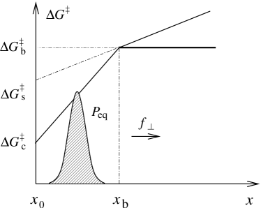
Figure 1: Schematic diagram of the height function of the energy barrier with respect to the coordinate $x$. $\Delta G^{\ddagger}_{s}$ and $\Delta G^{\ddagger}_{c}$ are the value of the linear functions in Eq. 42 at position $x_{0}$, while $\Delta G^{\ddagger}_{b}$ is the intersection of the functions at $x_{b}$. The bold solid line is the minimum model which is used to fit the experiment. The shaded area represents the equilibrium distribution of the conformational coordinate under the potential $V(y)$ ( Eq. 17).

In the constant force rupture experiment of the PSGL-1$-$P-selectin complex, the dissociation rate as the inverse mean lifetime of the complex first decreased and then increased when the applied force increased beyond a force threshold Marshall . We now can easily understand this counterintuitive transition according to the previous discussion about the Bell-like dissociation rate: the dissociation effect of $f_{\parallel}$ regains its dominance when the force is beyond the threshold. Although in principle we can construct various barrier height functions which result into catch-slip transitions, the most simplest form may be a composition of two linear functions

$$\Delta G^{\ddagger}(x)=\left\{\begin{gathered}\Delta G^{{\ddagger}}_{c}(x)=\Delta G^{{\ddagger}}_{b}+k_{c}(x-x_{b}),{\text{ }x\leq x_{b}}\hfill\\ \Delta G^{{\ddagger}}_{s}(x)=\Delta G^{{\ddagger}}_{b}+k_{s}(x-x_{b}),{\text{ }x>x_{b}}\hfill\\ \end{gathered}\right.$$ (42)

where we require that the distances defined in Eq. 36 with $k_{c}$ and $k_{s}$ are respectively minus and positive. For convenience, their absolute values are correspondingly denoted by $d^{\ddagger}_{c}$ and $d^{\ddagger}_{s}$. Define two “intrinsic” dissociation constants

$$k^{c}_{0}=k_{0}\exp[-\beta\Delta G^{\ddagger}_{c}(x_{0})],$$

$$k^{s}_{0}=k_{0}\exp[-\beta\Delta G^{\ddagger}_{s}(x_{0})].$$ (43)

Fig. 1 shows the characteristics of the function. We then have

$$\lambda_{0}(f) \approx \frac{k_{0}^{c}}{2}\exp\left[\frac{\beta k_{c}^{2}}{2k_{x}}\right]\exp\left[-\beta d^{\ddagger}_{c}f\right]$$

$$\times{\rm erfc}\left[-\left(\Delta+\frac{k_{c}}{k_{x}}\right)\sqrt{\frac{\beta k_{x}}{2}}+f\sqrt{\frac{\beta}{2k_{x}}}\sin\theta\right]$$

$$+\text{ }\frac{k_{0}^{s}}{2}\exp\left[\frac{\beta k_{s}^{2}}{2k_{x}}\right]\exp\left[\beta d^{\ddagger}_{s}f\right]$$

$$\times{\rm erfc}\left[\left(\Delta+\frac{k_{s}}{k_{x}}\right)\sqrt{\frac{\beta k_{x}}{2}}-f\sqrt{\frac{\beta}{2k_{x}}}\sin\theta\right]$$

where $\Delta=x_{b}-x_{0}$, and the complementary error function

$${\rm erfc}(x)=\frac{2}{\sqrt{\pi}}\int_{x}^{\infty}e^{-x^{2}}dx.$$ (45)

Before fixing numerical values of the parameters in Eq. II, we first simply analyze the main properties of $\lambda_{0}(f)$ given $\Delta\gg 0$: (i) in the absence of force, due to ${\rm erfc}(-\infty)=2$ and ${\rm erfc}(+\infty)=0$, we have

$$\lambda_{0}\approx k_{0}^{c}\exp(\beta k_{c}^{2}/2k_{x}),$$ (46)

which is the same with that obtained by Agmon and Hopfield Agmon ; (ii) if force is nonzero and smaller,

$$\lambda_{0}\approx k_{0}^{c}\exp(\beta k_{c}^{2}/2k_{x})\exp(-\beta d^{\ddagger}_{c}f),$$ (47)

which means that the bond is catch; and finally (iii), when the force is sufficiently large, Eq. II reduces to

$$\lambda_{0}\approx k_{0}^{s}\exp(\beta k_{s}^{2}/2k_{x})\exp(\beta d^{\ddagger}_{s}f).$$ (48)

It is the ordinary slip bond.

There are total eight independent parameters presenting in Eq. II: $\theta,\text{ }k_{x},\text{ }k_{c},\text{ }k_{s},\text{ }\Delta,\text{ }\xi^{\ddagger},\text{ }k_{0}$, and $\Delta G^{\ddagger}_{c}(x_{0})$. It is not necessary to determine all of them, which is also impossible only through fitting to the experimental data Marshall . For example, the latter two parameters are lumped into $k^{c}_{0}$, while and $\xi^{\ddagger}$ always presents with $\cos\theta$ together. What we really concern with is the coefficients of the force and the factors before the error functions in Eq. II. They can be obtained by least square fit. Guided by the properties Eqs 46 and 47, the fitting process in fact is simple. Even so, we are still able to fix all parameters from the fitting results if we study a minimum model in which the slop $k_{s}$ is zero and $\theta=\pi/6$. Here the particular value of the angle is actually of no particular significance and it is only as a reference. We immediately have: $k_{c}\approx 0.60\text{ pN}$, $k_{x}\approx 0.21\text{ pN nm}^{-1}$, $\xi^{\ddagger}\approx 0.25\text{ nm}$, $\Delta\approx 33\text{ nm}$; the other interesting parameters see Tab. 1, where the values are independent of the angle.

Table 1: Comparison of the parameters of the present theory, and the two-pathway and one energy-well model presented by Thomas et al. Pereverzev on the constant force (cf) and the dynamic force (df) modes. The parameters for the slip behavior of the P-selectin are also listed as a reference Hanley .

	$d_{c}$ nm	$d_{s}$ nm	$k_{0}^{c}$ sec-1	$k_{0}^{s}$ sec-1
Experiment		0.14		0.2
Dynamic disorder by us	1.2	0.22	23.2	1.68
Two-pathway one-well (cf)	2.2	0.5	120	0.25
Two-pathway one-well (df)	0.4	0.2	20	0.34

Substituting these values into Eq. II and according to Eq. 19, we calculate the mean lifetime of the PSGL-1$-$P-selectin complex with respect to different constant force in Fig. 2: the agreement between theory and the experimental data is quite good.

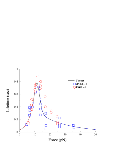
Figure 2: The mean lifetime as a function of force for the bonds of dimeric P-selectin with monomeric sPSGL-1 (square symbols) Marshall and the rescaled dimeric PSGL-1 (circle symbols) from Ref. Pereverzev . The two dash curves are respectively calculated by the two addition terms in Eq. II with the same parameters.

More challenging experiments to our theory are the force steady- and jump-ramp modes Evans2004 . Under large $D$ limitation, Eq. 27 reduces to

$$P(f,f_{0})\approx\frac{\lambda_{0}(f)}{r}\exp\left[-\frac{1}{r}\int_{f_{0}}^{f}\lambda_{0}(f^{\prime})df^{\prime}\right].$$ (49)

We see that the mean lifetime can be extracted from the above equation by setting $f=f_{0}$, i.e., $\langle\tau\rangle=1/rP(f_{0},f_{0})$. We calculate the dissociation force distributions of the steady- and jump-ramp modes at three loading rates to compare with the BFP experiments performed by Evans et al. Evans2004 . Here we are not ready to fit the experiments afresh; instead we directly apply the parameters obtained from the constant force mode to current case. Because the BFP experimental data is for dimeric ligand PSGL-1, whereas our parameters are from monomeric ligand sPSGL-1. Therefore it is necessary to map our predictions for the single bond sPSGL-1$-$P-selectin to the double bonds. A natural assumption is that the two bonds share the same force and fail randomly. The same assumption has been used in previous works Pereverzev ; Evans2004 . Hence, the probability density of the dissociation force for the double bond PSGL-1$-$P-selectin complex is related to the single case by

$$P_{\rm d}(f,f_{0})=P\left(f/2,f_{0}/2\right)^{2}.$$ (50)

Fig. 3 presents the final result. We see that the theoretical prediction agrees to the data very well. Hence we conclude that the adiabatic approximation proposed at the beginning is reasonable.

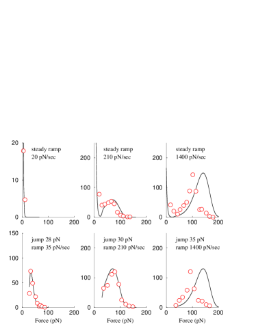
Figure 3: The probability density of the dissociation forces $P_{\rm d}(f,f_{0})$ under the different loading rates predicted by our theory (solid curves) for the PSGL-1$-$P-selectin complex. The symbols are from the force steady- and jump-ramp experimental data Evans2004 . The apparent deviations between the theory and the data in the last column may be from the invalidation of the assumption of two equivalent bonds at higher loading rates.

The previous works Evans2004 ; Pereverzev have claimed that they could not fit the experimental data from the constant force experiment using atomic force microscopy (AFM) and the force jump-ramp experiment using BFP with the same parameters, e.g., see Tab. 1. The authors simply contributed it to the different equipment and biological constructs though the experiments studied the same complexes Marshall ; Evans2004 . Our calculations however show that the mechanical parameters defined by us have almost the same values. In addition, the tendencies of our density functions for the first two panels of the second array in Fig. 3 are closer to the data than that predicted by the two-pathways models Evans2004 ; Pereverzev .

The density functions and the force histograms in the experiments reach the maximum and minimum at two distinct forces, which are named $f_{\rm min}$ and $f_{\rm max}$ in the following, respectively. This observation could be understood by setting the derivative of Eq. 27 with respect to $f$ equal to zero,

$$r\frac{d\lambda_{0}}{df}(f)=\lambda_{0}^{2}(f),$$ (51)

We immediately see that the values of $f_{\rm min}$ and $f_{\rm max}$ must be larger than the catch-slip transition force $f_{c}$ for the left term in Eq. 51 is negative as the bond is catch. Indeed the experimental observations show that the force values at the minimum histograms are around a certain values even the loading rates change 10-fold. (see Figs. 2 and 4 in Ref. Evans2004 ). The above equation could have no solutions when the loading rate is smaller than a critical rate $r_{c}$, which can be obtained by simultaneously solving Eq. 51 and its first derivative. We estimate $r_{\rm c}\approx 6$ pN/s using the current parameters, while the force $f_{\rm max}=f_{\rm min}\approx 13$ pN (about 26 pN in the double bond cases). If $r\leq r_{\rm c}$, then the density function is monotonous and decreasing function. Therefore, the most probable force at the bond dissociation is zero. The most interesting characteristics of Eq. 51 are the dependence of the maximum and minimum forces on the loading rate. In particular the latter is an important index in dynamic force spectroscopy (DFS) theory since it corresponds to the most possible dissociation force Evans01 . When the loading rate is sufficiently large, and correspondingly $f_{\rm max}$ is larger, the approximation of Eq. II at large force Eq. 47 implies that

$$f_{\rm max} \approx \frac{1}{\beta d_{s}}\ln\frac{\beta rd^{\ddagger}_{s}}{k_{0}^{s}\exp\left[\beta k_{s}^{2}/2k_{x}\right]}\propto\ln r.$$ (52)

The experimental measurement supported this prediction; see Fig. 3A in Ref. Evans2004 . On the other hand, due to that $f_{\rm min}$ is very close to $f_{c}$ at the larger loading rate, employing the Taylor’s expanding approach we have

$$\lambda_{0}(f)=\lambda_{0}(f_{c})+\frac{1}{2}\frac{d^{2}\lambda_{0}}{df^{2}}(f_{c})(\delta f)^{2}+o[(\delta f)^{3}],$$ (53)

where $\delta f=f-f_{c}$. Substituting it into Eq. 51, we get

$$f_{\rm min}\approx f_{c}+\lambda_{0}^{2}(f_{c})\left/r\frac{d^{2}\lambda_{0}}{df^{2}}(f_{c})\propto r^{-1}.\right.$$ (54)

It means that $f_{\rm min}$ tends to $f_{c}$ very fast. Different from $f_{\rm max}$, the loading rate dependence of $f_{\rm min}$ is an intrinsic property of the catch-slip bond; a unique requirement is that the dissociation rate $\lambda_{0}(f)$ has a minimum at the transition force $f_{c}$. Therefore $f_{\rm min}$s observed in experiment performed by Evans et al. Evans2004 are almost the catch-slip transition force observed in the constant force rupture experiment performed by Marshall et al. Marshall . Indeed, the force values of the minimum force histograms for the former are about 26 pN, while the transition force for the latter (dimeric PSGL-1$-$P-selectin) is also about 26 pN. We know that the dissociation forces distribution of a simple slip bond only has a maximum at a certain force value that depends on loading rate Izrailev . Therefor the catch-slip bond can easily be distinguished from the slip case by the presence of a minimum on the density function of the dissociation forces at a nonvanished force. Because the above analysis is independent of the initial force $f_{0}$, in order to track the catch behaviors in the force jump-ramp experiments, $f_{0}$ should be chosen to be smaller than $f_{c}$.

III Conclusions and discussion

Compared to the chemical kinetic schemes, our theory should be more attractive on the following aspects. First of all, we suggest that the counterintuitive catch-slip transition is a typical example of the rate processes with dynamic disorder. Because this concept has been broadly and deeply studied from theory and experiment during the past two decades, extensive experience and knowledge could be used for reference. For example, we suggest that a new receptor-ligand forced dissociation experiment could be performed over a large range of temperatures and solvent viscosities. According to Eq. 2, if the viscosity is so higher that $D\to 0$, we could predict

$$p(x,t)\approx p(x,0)\exp[-tk_{\rm off}(x,f_{\parallel})].$$ (55)

We know that such a dissociation reaction is a typical example of the rate processes with static disorder Zwanzig90 . In addition that the survival probability of the bond converts into multiple exponential decay at a single force from the single exponential decay at the large $D$ limitation (see Eq. 20), the mean lifetime is

$$\langle\tau\rangle\approx\int p(x,0)k^{-1}_{\rm off}(x,f_{\parallel}),$$ (56)

which means that the catch-slip bond changes into slip bond only. Then our theory gives a intuitively obvious physical explanation of catch bonds in an apparent expression (Eq. 35): they could arise from a competition of the two components of applied external force along the dissociation reaction coordinate and the molecular conformational coordinate; the former accelerates the dissociation by lowering the height of the energy barrier, while the latter stabilizes the complex by dragging the system to the higher barrier height. Finally, the time-dependence of the forced dissociation rates could be induced by either global conformational changes of the complex or local conformational changes at the interface between the receptor and ligand; no separated bound states and pathways are needed in the current theory. Therefore it is possible that one cannot find new stable complex structures through experiments or detailed molecular dynamics (MD) simulations.

Even there are many advantages in the present theory. We cannot definitely distinguish which theory or model is the most reasonable and more close real situations with existing experimental data. Moreover, except the coarse-grain physical picture our theory does not reveal the detailed structural information of the catch behavior of the ligand-receptor complexes, while biologists might be more interested in it. We could correspond the increasing height of the energy barrier with respect to the conformational coordinate to the hook structure Isberg or more affinity bound states Thomas , however we believe that further single-molecule experiments including micromanipulation experiments and fluorescence spectroscopy, more crystal structure data and detailed MD simulations from the atomic interactions are essential to elucidate the real molecular mechanism of the catch bonds.

FL thanks Prof. Mian Long and Dr. Fei Ye for their helpful discussion about the work.

References

- (1) McEver, R. P. (2002). Curr. Opin. Cell Biol. 14, 581-586.
- (2) Koonstantopoulos, K., Kurkreti, S. & McIntire, L. V. (1998) Adv. Drug Deliv. Rev. 33, 141-164.
- (3) Marshall, B. T., Long, M., Piper, J. W., Yago, T., McIver, R. P. & Zhu, C. (2003) Nature 423, 190-193
- (4) Evans, E., Leung, A., Heinrich, V., & Zhu, C. (2004) Proc. Natl. Acad. Sci. USA 101, 11281-11286.
- (5) Sarangapani, K. K., Yago, T., Klopocki, A. G., Lawrence, M. B., Fieger, C. B., Rosen, S. D., McEver, R. P. & Zhu, C. (2003) J. Biol. Chem. 279, 2291-2298.
- (6) Yago, T., Wu, J. H., Wey, C. D., Klopocki, A. G., Zhu, C., & McEver, R. P. (2004) J. Cell. Biol. 166, 913-923.
- (7) Marshall, B. T., Sarangapani, K. K., Lou, J. Z., McEver, R. P., & Zhu, C. (2005) Biophys. J. 88, 1458-1466.
- (8) Finger, E. B., Puri, K. D., Alon, R. Lawrence, M. B., von Andrian, U. H., & Springer, T. A. (1996) Nature 279, 266-269.
- (9) Lawrence, M. B., Kansas, G. S., Kunkel, E. J., & Ley, K. (1997) J. Cell. Biol. 136, 717-727.
- (10) Bell, G. I. (1978) Science 200, 618-627.
- (11) Alon, R., Hammer, D. A., & Springer, T. A. (1995) Nature 374, 539-542.
- (12) Chen, S. & Springer, T. A. (2003) Proc. Natl. Acad. Sci. USA 98, 950-955.
- (13) Dembo, M., Tourney, D. C., Saxman, K. & Hammer, D. (1988) Proc. R. Soc. Lond. B 234, 55-83.
- (14) Dembo, M. (1994) in Lectures on Mathematics in the Life Sciences: Some Mathematical Problems in Biology eds. Goldstein, B. & Wofsy, C. (Am. Mathematical Soc., Providence, RI) Vol. 25, pp. 1-27.
- (15) Evans, E. & Ritchie, K. (1997) Biophys. J. 72, 1541-1555.
- (16) Barsegov, V. & Thirumalai, D. (2005) Proc. Natl. Acad. Sci. USA 102, 1835-1840.
- (17) Pereverzev, Y. V., Prezhdo, O. V., Forero, M., Sokurenko, E. V., & Thomas, W. (2005) Biophys. J. 89, 1446-1454.
- (18) Somers, W. S., Tang, J., Shaw, G. D., & Camphausen, R. T. (2000) Cell 103, 467-479.
- (19) Zwanzig, R. (1990) Acc. Chem. Res. 23, 148-152.
- (20) Agmon, N. & Hopfield, J. J. (1983) J. Chem. Phys. 78, 6947-6959.
- (21) Van Kampen, N. G. J. Stat. Phys. (1977) 17, 71-80.
- (22) Messiah, A. Quantum mechanics (North-Holland Pub. Co. Amsterdam, 1962)
- (23) Hanley, W., McCarty, O. Jadhav, S., Tseng, Y., Wirtz, D. & Konstantopoulos, K. (2003) J. Biol. Chem. 278, 10556-10561.
- (24) Evans, E. A. (2001) Annu. Rev. Biophys. Biomol. Struct. 30, 105-128.
- (25) Izrailev, S., Stepaniants, s., Balsera, M., Oono, Y., & Schulten, K. (1997) Biophys. J. 72, 1568-1581.
- (26) Isberg, R. R. & Barnes, P. (2002) Cell 110, 1-4.
- (27) Thomas, W. E., Trintchina, E., Forero, M., Vogel, V., & Sokurenko, E. V. (2002) Cell 109, 913-923.