Connectivity and expression in protein networks:
Proteins in a complex are uniformly expressed

Abstract

We explore the interplay between the protein-protein interactions network and the expression of the interacting proteins. It is shown that interacting proteins are expressed in significantly more similar cellular concentrations. This is largely due to interacting pairs which are part of protein complexes. We solve a generic model of complex formation and show explicitly that complexes form most efficiently when their members have roughly the same concentrations. Therefore, the observed similarity in interacting protein concentrations could be attributed to optimization for efficiency of complex formation.

I Introduction

Statistical analysis of real-world networks topology has attracted much interest in recent years, proving to supply new insights and ideas to many diverse fields. In particular, the protein-protein interaction network, combining many different interactions of proteins within a cell, has been the subject of many studies (for a recent review see Barabasi ). While this network shares many of the universal features of natural networks such as the scale-free distribution of degrees Jeong , and the small world characteristics flag , it also has some unique features. One of the most important of these is arguably the fact that the protein interactions underlying this network can be separated into two roughly disjoint classes. One of them relates to transmission of information within the cell: protein A interacts with protein B and changes it, by a conformational or chemical transformation. The usual scenario after such an interaction is that the two proteins disassociate shortly after the completion of the transformation. On the other hand, many protein interactions are aimed at the formation of a protein complex. In this mode of operation the physical attachment of two or more proteins is needed in order to allow for the biological activity of the combined complex, and is typically stable over relatively long time scales Han .

The yeast Saccharomyces cerevisiae serves as the model organism for most of the analyses of protein-protein interaction network. The complete set of genes and proteins with extensive data on gene expression are available Cherry for this unicellular organism, accompanied by large datasets of protein-protein interactions based on a wide range of experimental and computational methods synexp ; mrna ; genefus ; hms ; y2h ; synleth ; 2nei ; tap ; von Mering . In addition, the intracellular locations and the expression levels of most proteins of the yeast were recently reported Ghaemmaghami . The availability of such data enables us to study the relationship between network topology and the expression levels of each protein.

In this work we demonstrate the importance of the distinction between different types of protein interaction, by highlighting one property which is unique to interactions of the protein complexes. Combining databases of yeast protein interactions with the recently reported information on the protein concentration, we find that proteins belonging to the same complex tend to have a more uniform concentration distribution. We further explain this finding by a model of complex formation, showing that uneven concentrations of the complex members result in inefficient complex formation. Surprisingly, in some cases increasing the concentration of one of the complex ingredients decreases the absolute number of complexes formed. Thus, the experimental observation of uniform complex members concentrations can be explained in terms of selection for efficiency.

II Concentrations of Interacting Proteins

We start by studying the concentrations of pairs of interacting proteins, and demonstrate that different types of protein-protein interactions differ in their properties. For this purpose we use the recently published database providing the (average) concentration Ghaemmaghami , as well as the localization within the cell, for most of the Saccharomyces cerevisiae (baker’s yeast) proteins Huh . The concentrations $c_{i}$ (given in arbitrary units) are approximately distributed according to a log-normal distribution with $\langle log(c_{i})\rangle=7.89$ and standard deviation $1.53$ (Fig. 1).

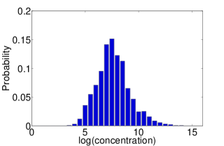
Figure 1: (Color online) Distribution of the logarithm of the protein concentration (in units of protein molecules per cell) for all measured proteins within the yeast cell.

The bakers’ yeast serves as a model organism for most of the protein-protein interaction network studies. Thus a set of many of its protein-protein interactions is also readily available. Here we use a dataset of recorded yeast protein interactions, given with various levels of confidence von Mering . The dataset lists about $80000$ interactions between approximately $5300$ of the yeast proteins (or about $12000$ interactions between $2600$ proteins when excluding interactions of the lowest confidence). These interactions were deduced by many different experimental methods, and describe different biological relations between the proteins involved. The protein interaction network exhibits a high level of clustering (clustering coefficient $\approx 0.39$). This is partly due to the existence of many sets of proteins forming complexes, where each of the complex members interacts with many other members.

Combining these two databases, we study the correlation between the (logarithm of) concentrations of pairs of interacting proteins. In order to gain insight into the different components of the network, we perform this calculation separately for the interactions deduced by different experimental methods. For simplicity, we report here the results after excluding the interactions annotated as low-confidence (many of which are expected to be false-positives). We have explicitly checked that their inclusion does not change the results qualitatively. The results are summarized in Table 1, and show a significant correlation between the expression levels of interacting proteins.

Interaction	Number of	Number of	Number of	Correlation	STD of	P-Value
	interacting	interactions	interactions in	between	random
	proteins		which expression	expression	correlations
			level is	levels of
			known for	interacting
			both proteins	proteins
All	2617	11855	6347	0.167	0.012	$10^{-42}$
Synexpressionsynexp ; mrna	260	372	200	0.4	0.065	$3.5\cdot 10^{-10}$
Gene Fusiongenefus	293	358	174	-0.079	-	-
HMShms	670	1958	1230	0.164	0.027	$3.3\cdot 10^{-10}$
yeast 2-Hybridy2h	954	907	501	0.097	0.046	$1.7\cdot 10^{-2}$
Synthetic Lethalitysynleth	678	886	497	0.285	0.045	$1.2\cdot 10^{-10}$
2-neighborhood2nei	998	6387	3110	0.054	0.016	$5.4\cdot 10^{-4}$
TAPtap	806	3676	2239	0.291	0.02	$10^{-49}$

Table 1: (Color online) Correlation coefficients between the logarithm of the concentrations of interacting proteins. Only interactions of medium or high confidence were included. The statistical significance of the results was estimated by randomly permuting the concentrations of the proteins and reevaluating the correlation on the same underlying network, repeated for 1,000 different permutations. The mean correlation of the randomly permuted networks was zero, and the standard deviation (STD) is given. The P-value was calculated assuming gaussian distribution of the correlation values for the randomized networks. We have verified that the distributions of the 1,000 realizations calculated are roughly Guassian.

The strongest correlation is seen for the subset of protein interactions which were derived from synexpression, i.e. inferred from correlated mRNA expression. This result confirms the common expectation that genes with correlated mRNA expression would yield correlated protein levels as wellmrna . However, our results show that interacting protein pairs whose interaction was deduced by other methods exhibit significant positive correlation as well. The effect is weak for the yeast 2-Hybrid (Y2H) methody2h which includes all possible physical interactions between the proteins (and is also known to suffer from many artifacts and false-positives), but stronger for the HMS (High-throughput Mass Spectrometry)hms and TAP (Tandem-Affinity Purification)tap interactions corresponding to actual physical interactions (i.e., experimental evidence that the proteins actually bind together in-vivo). These experimental methods are specifically designed to detect cellular protein complexes. The above results thus hint that the overall correlation between concentrations of interacting proteins is due to the tendency of proteins which are part of a stable complex to have similar concentrations.

The same picture emerges when one counts the number of interactions a protein has with other proteins of similar concentration, compared to the number of interactions with randomly chosen proteins. A protein interacts, on average, with $0.49\%$ of the proteins with similar expression level (i.e., $|$log-difference$|<1$), as opposed to only $0.36\pm 0.01~{}\%$ of random proteins, in agreement with the above observation of complex members having similar protein concentrations.

In order to directly test this hypothesis (i.e. that proteins in a complex have similar concentrations), we use existing datasets of protein complexes and study the uniformity of concentrations of members of each complex. The complexes data were taken from complexes , and were found to have many TAP interactions within them. As a measure of the uniformity of the expression levels within each complex, we calculate the variance of the (logarithm of the) concentrations among the members of each complex. The average variance (over all complexes) is found to be $2.35$, compared to $2.88\pm 0.07$ and $2.74\pm 0.11$ for randomized complexes in two different randomization schemes (see figure), confirming that the concentrations of complex members tend to be more uniform than a random set of proteins.

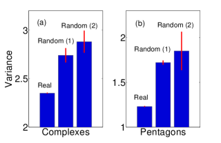
Figure 2: (Color online) (a) Variance of the logarithm of the protein expression levels (in units of mulecules per cell) for members of real complexes, averaged over all complexes, comapred with the averaged variance of the complexes after randomization of their members, letting each protein participate on average in the same number of complexes (random(1)), as well as randomized complexes where the number of complexes each protein participates in is kept fixed (random(2)). Real complexes have a lower variance, indicating higher uniformity in the expression levels of the underlying proteins. (b) Same as (a) for expression levels in pentagons (see text).

As another test, we study a different yeast protein interaction network, the one from the DIP database Xenarios . We look for fully-connected sub-graphs of size $5$, which are expected to represent complexes, sub-complexes or groups of proteins working together. The network contains approximately $1600$ (highly overlapping) such pentagons, made of about $300$ different proteins. The variance of the logarithm of the concentrations of each pentagon members, averaged over the different pentagons, is 1.234. As before, this is a significantly low variance compared with random sets of five proteins (average variance $1.847\pm 0.02$ and $1.718\pm 0.21$), see figure 2.

Finally, we have used mRNA expression data mrna and looked for correlated expression patterns within complexes. We have calculated the correlation coefficient between the expression data of the two proteins for each pair of proteins which are part of the same pentagon. The average correlation coefficient between proteins belonging to the same fully-connected pentagon is $0.15$ compared to $0.056\pm 0.005$ for a random pair.

In summary, combination of a number of yeast protein interaction networks with protein and mRNA expression data yields the conclusion that interacting proteins tend to have similar concentrations. The effect is stronger when focusing on interactions which represent stable physical interactions, i.e. complex formation, suggesting that the overall effect is largely due to the uniformity in the concentrations of proteins belonging to the same complex. In the next Section we explain this finding by a model of complex formation. We show, on general grounds, that complex formation is more effective when the concentrations of its constituents is roughly the same. Thus, the observation made in the present Section can be explained by selection for efficiency of complex formation.

III Model

Here we study a model of complex formation, and explore the effectiveness of complex production as a function of the relative abundances of its constituents. For simplicity, we start by a detailed analysis of the three-components complex production, which already captures most of the important effects.

Denote the concentrations of the three components of the complex by $A$, $B$ and $C$, and the concentrations of the complexes they form by $AB$, $AC$, $BC$ and $ABC$. The latter is the concentration of the full complex, which is the desired outcome of the production, while the first three describe the different sub-complexes which are formed (in this case, each of which is composed of two components). Three-body processes, i.e., direct generation (or decomposition) of $ABC$ out of $A$ $B$ and $C$, can usually be neglected book , but their inclusion here does not complicate the analysis. The resulting set of reaction kinetic equations is given by

$$\frac{d(A)}{dt} = k_{d_{A,B}}AB+k_{d_{A,C}}AC+(k_{d_{A,BC}}+k_{d_{A,B,C}})\cdot ABC$$ (1)

$$-k_{a_{A,B}}A\cdot B-k_{a_{A,C}}A\cdot C-k_{a_{A,BC}}A\cdot BC-k_{a_{A,B,C}}A\cdot B\cdot C$$

$$\frac{d(B)}{dt} = k_{d_{A,B}}AB+k_{d_{B,C}}BC+(k_{d_{B,AC}}+k_{d_{A,B,C}})\cdot ABC$$ (2)

$$-k_{a_{A,B}}A\cdot B-k_{a_{B,C}}B\cdot C-k_{a_{B,AC}}B\cdot AC-k_{a_{A,B,C}}A\cdot B\cdot C$$

$$\frac{d(C)}{dt} = k_{d_{A,C}}AC+k_{d_{B,C}}BC+(k_{d_{C,AB}}+k_{d_{A,B,C}})\cdot ABC$$ (3)

$$-k_{a_{A,C}}A\cdot C-k_{a_{B,C}}B\cdot C-k_{a_{C,AB}}C\cdot AB-k_{a_{A,B,C}}A\cdot B\cdot C$$

$$\frac{d(AB)}{dt} = k_{a_{A,B}}A\cdot B+k_{d_{C,AB}}ABC-k_{d_{A,B}}AB-k_{a_{C,AB}}C\cdot AB$$ (4)

$$\frac{d(AC)}{dt} = k_{a_{A,C}}A\cdot C+k_{d_{B,AC}}ABC-k_{d_{A,C}}AC-k_{a_{B,AC}}B\cdot AC$$ (5)

$$\frac{d(BC)}{dt} = k_{a_{B,C}}B\cdot C+k_{d_{A,BC}}ABC-k_{d_{B,C}}BC-k_{a_{A,BC}}A\cdot BC$$ (6)

$$\frac{d(ABC)}{dt} = k_{a_{A,BC}}A\cdot BC+k_{a_{B,AC}}B\cdot AC+k_{a_{C,AB}}C\cdot AB+k_{a_{A,B,C}}A\cdot B\cdot C$$ (7)

$$-(k_{d_{A,BC}}+k_{d_{B,AC}}+k_{d_{C,AB}}+k_{d_{A,B,C}})\cdot ABC$$

where $k_{a_{x,y}}$ ($k_{d_{x,y}}$) are the association (dissociation) rates of the subcomponents $x$ and $y$ to form the complex $xy$. Denoting the total number of type $A$, $B$ and $C$ particles by $A_{0}$, $B_{0}$, $C_{0}$, respectively, we may write the conservation of material equations:

$$A+AB+AC+ABC=A_{0}$$ (8)

$$B+BC+AB+ABC=B_{0}$$ (9)

$$A+AC+BC+ABC=C_{0}$$ (10)

We look for the steady-state solution of these equations, where all time derivatives vanish. For simplicity, we consider first the totally symmetric situation, where all the ratios of association coefficients to their corresponding dissociation coefficients are equal, i.e., the ratios $k_{d_{x,y}}/k_{a_{x,y}}$ are all equal to $X_{0}$ and $k_{d_{x,y,z}}/k_{a_{x,y,z}}=X_{0}^{2}$, where $X_{0}$ is a constant with concentrations units. In this case, measuring all concentrations in units of $X_{0}$, all the reaction equations are solved by the substitutions $AB=A\cdot B$, $AC=A\cdot C$, $BC=B\cdot C$ and $ABC=A\cdot B\cdot C$, and one needs only to solve the material conservation equations, which take the form:

$$A+A\cdot B+A\cdot C+A\cdot B\cdot C=A_{0}$$ (11)

$$B+B\cdot C+A\cdot B+A\cdot B\cdot C=B_{0}$$ (12)

$$A+A\cdot C+B\cdot C+A\cdot B\cdot C=C_{0}$$ (13)

These equations allow for an exact and straight-forward (albeit cumbersome) analytical solution. In the following, we explore the properties of this solution. The efficiency of the production of $ABC$, the desired complex, can be measured by the number of formed complexes relative to the maximal number of complexes possible given the initial concentrations of supplied particles ${\rm eff}\equiv ABC/\min{(A_{0},B_{0},C_{0})}$. This definition does not take into account the obvious waste resulting from proteins of the more abundant species which are bound to be leftover due to shortage of proteins of the other species. In the following we show that having unmatched concentrations of the different complex components result in lower efficiency beyond this obvious waste.

In the linear regime, $A_{0},B_{0},C_{0}\ll 1$, the fraction of particles forming complexes is small, and all concentrations are just proportional to the initial concentrations. The overall efficiency of the process in this regime is extremely low, $ABC=A\cdot B\cdot C\sim A_{0}\cdot B_{0}\cdot C_{0}\ll A_{0},B_{0},C_{0}$. We thus go beyond this trivial linear regime, and focus on the region where all concentrations are greater than unity. Fig. 3 presents the efficiency as a function of $A_{0}$ and $B_{0}$, for fixed $C_{0}=10^{2}$. The efficiency is maximized when the two more abundant components have approximately the same concentration, i.e., for $A_{0}\approx B_{0}$ (if $C_{0}<A_{0},B_{0}$), for $A_{0}\approx C_{0}=10^{2}$ (if $B_{0}<A_{0},C_{0}$) and for $B_{0}\approx C_{0}=10^{2}$ (if $A_{0}<B_{0},C_{0}$).

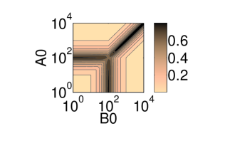
Figure 3: (Color online) The efficiency of the synthesis ${\rm eff}\equiv ABC/\min{(A_{0},B_{0},C_{0})}$ as a function of $A_{0}$ and $B_{0}$, for $C_{0}=10^{2}$. The efficiency is maximized when the two most abundant species have roughly the same concentration.

Moreover, looking at the absolute quantity of the complex product, one observes (fixing the concentrations of two of substances, e.g., $B_{0}$ and $C_{0}$) that $ABC$ itself has a maximum at some finite $A_{0}$, i.e., there is a finite optimal concentration for $A$ particles (see Fig. 4). Adding more molecules of type $A$ beyond the optimal concentration decreases the amount of the desired complexes. The concentration that maximizes the overall production of the three-component complex is $A_{0,max}\approx\max{(B_{0},C_{0})}$.

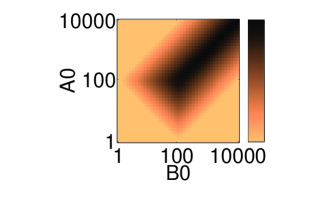
Figure 4: (Color online) $\log{(ABC)}$ as a function of $A_{0},B_{0}$, for fixed $C_{0}=10^{2}$. For each row (fixed $A_{0}$) or column (fixed $B_{0}$) in the graph, $ABC$ has a maximum, which occurs where $A_{0,max}\approx\max{(B_{0},C_{0})}$ (for columns), and $B_{0,max}\approx\max{(A_{0},C_{0})}$ (for rows).

An analytical solution is available for a somewhat more general situation, allowing the ratios $k_{d_{x,y}}/k_{a_{x,y}}$ to take different values for the two-components association/dissociation ($X_{0}$) and the three-components association/dissociation ($X_{0}/\alpha$ and $X_{0}^{2}/\alpha$ for association/dissociation of the three-component complex from/to a two-component complex plus one single particle or to three single particles, respectively). It can be easily seen that under these conditions, and measuring the concentration in units of $X_{0}$ again, the solution of the reaction kinetics equations is given by

$$AB = A\cdot B,$$ (14)

$$AC = A\cdot C,$$ (15)

$$BC = B\cdot C,$$ (16)

$$ABC = \alpha~{}A\cdot B\cdot C,$$ (17)

and therefore the conservation of material equations take the form

$$A+A\cdot B+A\cdot C+\alpha A\cdot B\cdot C=A_{0}$$ (18)

$$B+B\cdot C+A\cdot B+\alpha A\cdot B\cdot C=B_{0}$$ (19)

$$A+A\cdot C+B\cdot C+\alpha A\cdot B\cdot C=C_{0}$$ (20)

These equations are also amenable for an analytical solution, and one finds that taking $\alpha$ not equal to $1$ does not qualitatively change the above results. In particular, the synthesis is most efficient when the two highest concentrations are roughly equal, see Fig. 5. Note that our results hold even for $\alpha\gg 1$, where the three-component complex is much more stable than the intermediate $AB$, $AC$, and $BC$ states.

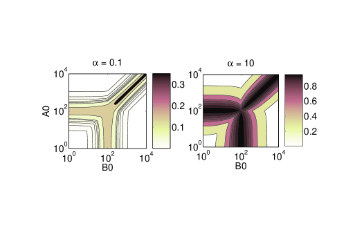
Figure 5: (Color online) Synthesis efficiency ${\rm eff}\equiv ABC/\min{(A_{0},B_{0},C_{0})}$ as a function of $A_{0}$ and $B_{0}$, for different values of $\alpha$. $C_{0}$ is fixed, $C_{0}=100$. The efficiency is maximized when the two most abundant substances are of roughly the same concentration, regardless of the values of $\alpha$.

We have explicitly checked that the same picture holds for 4-component complexes as well: fixing the concentrations $B_{0}$, $C_{0}$, and $D_{0}$, the concentration of the target complex $ABCD$ is again maximized for $A_{0,max}\approx\max{(B_{0},C_{0},D_{0})}$. This behavior is expected to hold qualitatively for a general number of components and arbitrary reaction rates, due to the following argument: Assume a complex is to be produced from many constituents, one of which ($A$) is far more abundant than the others ($B$, $C$, …). Since $A$ is in excess, almost all $B$ particles will bound to $A$ and form $AB$ complexes. Similarly, almost all $C$ particles will bound to $A$ to form an $AC$ complex. Thus, there will be very few free $C$ particles to bound to the $AB$ complexes, and very few free $B$ particles available for binding with the $AC$ complexes. As a result, one gets relatively many half-done $AB$ and $AC$ complexes, but not the desired $ABC$ (note that $AB$ and $AC$ cannot bound together). Lowering the concentration of $A$ particles allows more $B$ and $C$ particles to remain in an unbounded state, and thus increases the total production rate of $ABC$ complexes (Fig. 6).

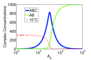
Figure 6: (Color online) The dimensionless concentrations of the complex $ABC$ (solid line), partial complex $AB$ (dashed line), and $C$ (dotted line) as a function of the total concentration of $A$ particles, $A_{0}$ ($C$ is multiplied by 10 for visibility). $B_{0}$ and $C_{0}$ are fixed $B_{0}=C_{0}=10^{3}$. The maximum of $ABC$ for finite $A_{0}$ is a result of the balance between increase in the number of $AB$ and $AC$ complexes and the decrease in the number of available free $B$ and $C$ particles as $A_{0}$ increases.

Many proteins take part in more than one complex. One might thus wonder what is the optimal concentration for these, and how it affects the general correlation observed between the concentrations of members of the same complex. In order to clarify this issue, we have studied a model in which four proteins $A$, $B$, $C$ and $D$ bind together to form two desired products: the $ABC$ and $BCD$ complexes. $A$ and $D$ do not interact, so that there are no complexes or sub-complexes of the type $AD$, $ABD$, $ACD$ and $ABCD$. Solution of this model (see appendix) reveals that the efficiency of the production of $ABC$ and $BCD$ is maximized when (for a fixed ratio of $A_{0}$ and $D_{0}$) $A_{0}+D_{0}\approx B_{0}\approx C_{0}$. One thus sees, as could have been expected, that proteins that are involved in more than one complex (like $B$ and $C$ in the above model) will tend to have higher concentrations than other members of the same complex participating in only one complex. Nevertheless, since the protein-protein interaction network is scale-free, most proteins take part in a small-number of complexes, and only a very small fraction participate in many complexes. Moreover, given the three orders of magnitude spread in protein concentrations (see figure 1), only proteins participating in a very large number of complexes (relative to the avregae participation) or participating in two complexes of a very different concentrations (i.e., $A_{0}\gg D_{0}$) will result in order-of-magnitude deviations from the equal concentration optimum. The effects of these relatively few proteins on the average over all interacting proteins is small enough not to destroy the concentration correlation, as we observed in the experimental data.

In summary, the solution of our simplified complex formation model shows that the rate and efficiency of complex formation depends strongly, and in a non-obvious way, on the relative concentrations of the constituents of the complex. The efficiency is maximized when all concentrations of the different complex constituents are roughly equal. Adding more of the ingredients beyond this optimal point not only reduces the efficiency, but also results in lower product yield. This unexpected behavior is qualitatively explained by a simple argument, and is expected to hold generally. Therefore, effective formation of complexes in a network puts constraints on the concentrations on the underlying building blocks. Accordingly, one can understand the tendency of members of cellular protein-complexes to have uniform concentrations, as presented in the previous Section, as a selection towards efficiency.

*

Appendix A Two coupled complexes

We consider a model in which four proteins $A$, $B$, $C$ and $D$ bind together to form two desired products: the $ABC$ and $BCD$ complexes. $A$ and $D$ do not interact, so that there are no complexes or sub-complexes of the type $AD$, $ABD$, $ACD$ and $ABCD$. For simplicity, we assume the totally symmetric situation, where all the ratios of association coefficients to their corresponding dissociation coefficients are equal, i.e., the ratios $k_{d_{x,y}}/k_{a_{x,y}}$ are all equal to $X_{0}$ and $k_{d_{x,y,z}}/k_{a_{x,y,z}}=X_{0}^{2}$, where $X_{0}$ is a constant with concentrations units. The extension to the more general case discussed in the paper is straight forward. Using the same scaling as above, the reaction equations are solved by the substitutions $AB=A\cdot B$, $AC=A\cdot C$, $BC=B\cdot C$, $BD=B\cdot D$, $CD=C\cdot D$, $ABC=A\cdot B\cdot C$, and $BCD=B\cdot C\cdot D$, and one needs only to solve the material conservation equations, which take the form:

$$A +A\cdot B+A\cdot C+A\cdot B\cdot C=A_{0}$$

$$B +A\cdot B+B\cdot C+B\cdot D+A\cdot B\cdot C+B\cdot C\cdot D=B_{0}$$

$$C +A\cdot C+B\cdot C+C\cdot D+A\cdot B\cdot C+B\cdot C\cdot D=C_{0}$$

$$D +B\cdot D+C\cdot D+B\cdot C\cdot D=D_{0}$$ (24)

Denoting $\gamma\equiv\frac{D_{0}}{A_{0}},D^{\prime}\equiv\frac{D}{\gamma}$, Eq (24) becomes

$$D^{\prime}+D^{\prime}\cdot B+D^{\prime}\cdot C+D^{\prime}\cdot B\cdot C=A_{0}$$ (25)

This is exactly the equation we wrote for A (A), and thus $D=\gamma A$. Substitutng this into equations (LABEL:eqB) and (LABEL:eqC), one gets

$$B+B\cdot C+(\gamma+1)A\cdot B+(\gamma+1)A\cdot B\cdot C=B_{0}$$ (26)

$$C+B\cdot C+(\gamma+1)A\cdot C+(\gamma+1)A\cdot B\cdot C=C_{0}$$ (27)

We now define $A^{\prime}\equiv(\gamma+1)A$, $A^{\prime}_{0}\equiv(\gamma+1)A_{0}$ and obtain from (A,26,27)

$$A^{\prime}+A^{\prime}\cdot B+A^{\prime}\cdot C+A^{\prime}\cdot B\cdot C = A^{\prime}_{0}$$ (28)

$$B+A^{\prime}\cdot B+B\cdot C+A^{\prime}\cdot B\cdot C = B_{0}$$ (29)

$$C+A^{\prime}\cdot C+B\cdot C+A^{\prime}\cdot B\cdot C = C_{0}$$ (30)

These are the very same equations that we wrote for the 3-particles case where the desired product was $ABC$. Their solution showed that efficiency is maximized at $A_{0}\approx B_{0}\approx C_{0}$. We thus conclude that in the present 4-component scenario, the efficiency of $ABC$ and $BCD$ (for fixed $\gamma$) is maximized when $(A_{0}+D_{0})\approx B_{0}\approx C_{0}$.

- (1) A.L. Barabasi and Z.N. Oltvai, Nat Rev Genet 5, 101 (2004).
- (2) H. Jeong et al, Nature 411, 41 (2001).
- (3) S.H. Yook, Z.N. Oltvai and A.L. Barabasi, Proteomics 4, 928 (2004).
- (4) J.D. Han et al, Nature 430, 88 (2004).
- (5) J.M. Cherry et al, Nature 387, 67 (1997).
- (6) R.J. Cho et al,Mol. Cell 2, 65 (1998).
- (7) T.R. Hughes et al, Cell 102, 109 (2000).
- (8) A.J. Enright, I. Iliopoulos, N.C. Kyrpides, and C.A. Ouzounis, Nature 402, 86 (1999); E.M. Marcotte et al, Science 285, 751 (1999).
- (9) Y. Ho et al, Nature 415, 180 (2002).
- (10) P. Uetz et al, Nature 403, 623 (2000); T. Ito et al, Proc. Natl Acad. Sci. USA 98, 4569 (2001).
- (11) A.H. Tong et al, Science 294, 2364 (2001).
- (12) R. Overbeek et al. Proc. Natl Acad. Sci. USA 96, 2896 (1999).
- (13) A.C. Gavin et al, Nature 415, 141 (2002).
- (14) C. von Mering et al, Nature 417, 399 (2002).
- (15) S. Ghaemmaghami et al, Nature 425, 737 (2003).
- (16) W.K. Huh et al, Nature 425, 686 (2003).
- (17) H. W. Mewes et al, Nucleic Acids Res. 30, 31 (2002).
- (18) I. Xenarios et al, Nucleic Acids Res. 29, 239 (2001).
- (19) See, e.g., P.L. Brezonik, Chemical Kinetics and Process Dynamics in Aquatic Systems, Lewis Publishers, 1993 Boca Raton, FL, USA.