Turing pattern with proportion preservation

Shuji Ishihara¹ and Kunihiko Kaneko^1,2

¹Department of Pure and Applied Sciences, University of Tokyo, Komaba, Meguro-ku, Tokyo 153-8902, Japan
² ERATO Complex Systems Biology Project, JST

Correspondence should be addressed to S. Ishihara
E-mail : shuji@complex.c.u-tokyo.ac.jp
Department of Pure and Applied Sciences, College of Arts and Sciences,
The University of Tokyo, 3-8-1 Komaba, Meguro-ku, Tokyo 153-8902, Japan.
Tel/Fax : +81-3-5454-6731

Although Turing pattern is one of the most universal mechanisms for pattern formation, in its standard model the number of stripes changes with the system size, since the wavelength of the pattern is invariant: It fails to preserve the proportionality of the pattern, i.e., the ratio of the wavelength to the size, that is often required in biological morphogeneis. To get over this problem, we show that the Turing pattern can preserve proportionality by introducing a catalytic chemical whose concentration depends on the system size. Several plausible mechanisms for such size dependence of the concentration are discussed. Following this general discussion, two models are studied in which arising Turing patterns indeed preserve the proportionality. Relevance of the present mechanism to biological morphogenesis is discussed from the viewpoint of its generality, robustness, and evolutionary accessibility.

Keywords : Turing pattern; Morphogenesis; size-invariance

1 Introduction

Since the seminal paper by Turing (1952), a large variety of pattern formation phenomena in nature has been explained by his theory. The original motivation of Turing himself lied in the explanation of biological morphogenesis, as was succeeded to Gierer and Meinhardt (Gierer and Meinhardt, 1972), and others over a half century (Gray and Scott, 1984; Murray 1993; Pearson, 1993; Kondo and Asai, 1995; Meinhardt and Gierer, 2000). Although the Turing pattern is one of the most beautiful and ubiquitous mechanisms for morphogenesis, frequent criticism raised to it is non-adjustability of the characteristic wave length of the pattern against the system size. Because the generation of the Turing pattern comes from instability of an uniform state over a certain range of wavelengths, the possible range of the wavelengths is pre-fixed, and is invariant against the change of the system size. Hence the number of segments or stripes is proportional to the system size as shown in Fig. 1 (a). In contrast, the number of segments or stripes, rather than the wavelength, is often invariant against the change of the size in many biological systems as shown in Fig. 1 (b). In a biological system, the scale of pattern is often proportional to the system size, and also it is desirable to have such proportionality in many situations. However, neither the Turing pattern nor the positional information theory by Wolpert (1969) which assumes the morphogen gradient to convey positional information satisfies the scale-invariance.

For example, it is observed that the patterns in Hydra and Dictyostelium discoideum slugs have proportionality with the size. In Dictyostelium discoideum the ratio of two different cell types is almost fixed, independent of the size. Transgenic mice indeed preserve the body proportion despite their larger size in phenotype (Palmiter et al., 1982). In the development of Drosophila Melanogaster, it was reported that the expression of gap gene hb is robust and preserves the proportion over different sizes of individual eggs (Houchmandzadeh et al., 2002). The proportion preservation is important for robust morphogenesis in general.

In the present paper we discuss a general mechanism which enables the proportionality of wavelength with the size in Turing patterns as in Fig. 1 (b).

To explain the proportion regulation of different cell types for Dictyostelium discoideum slug, Meinhardt (1982) proposed an activator-inhibitor model in which the ratio of two cell types is preserved. The mechanism works well for a pattern with only a single boundary between two types, but is not valid for multiple stripes pattern. Theory based on globally coupled dynamical systems also provides a regulation mechanism for the ratio of different cell types (Kaneko and Yomo, 1994, 1999; Mizuguchi and Sano, 1995; Furusawa and Kaneko, 2001), but a proportion preservation of a pattern with multiple stripes is not discussed yet.

As an extension of Turing pattern, Othmer and Pate (1980) showed that if diffusion constants depend on the concentration of auxiliary chemical factor which has size-dependence, then size-invariant pattern formation is possible, where the size-dependence of the auxiliary chemical concentration is provided by choosing a proper boundary condition (see also Pate and Othmer, 1984; Dillon et al., 1994). Hunding and Sørensen (1988) also discussed a simple mechanism to explain such concentration-dependent diffusion by an auxiliary chemical factor. In these models, it is necessary that all the diffusion coefficients are regulated in the same manner. Apart from Turing pattern, a model for the proportion regulation in Drosophila Melanogaster was proposed by Aegerter-Wilmsen et al. (2005), also by assuming effectively concentration-dependent diffusion. It is not yet sure if such regulation of diffusion is really adopted to control the proportionality.

In this paper we discuss mechanisms of scale-invariant Turing pattern without considering any variations of diffusion constants. Instead we seek for a possibility that concentration of some chemical changes with some power of the system size, which influences the rate of reaction for the Turing pattern so that the size-invariance is generated. We introduce a chemical component whose concentration depends on the size of the system. In Section 2 we discuss several possibilities for such size-dependent concentration of a chemical. Following this general discussion, we give two specific examples leading to the Turing pattern whose wavelength is proportional to the system size. The first example introduced in Section 3 adopts a size-dependent auxiliary chemical component, in the same way as Othmer and Pate (1980) or Hunding and Sørensen (1988), while we believe it is simpler than the earlier models, and is also plausible biologically because change between active and inactive forms adopted therein is ubiquitous in a biochemical process. The second example introduced in Section 4 contains only two chemical components, which is the minimum number for the Turing instability. The model provides a novel mechanism for the proportionality preservation based on the conservation of some quantity. Due to the size dependence of the conserved quantity, the scale-invariance in Turing pattern is resulted. In Section 5 we summarize the mechanisms for the proportion preservation and discuss possible relevance of them to biological morphogenesis.

Before discussing the mechanisms, we make one remark what we have in mind with the term “system” in the present paper. In a class of examples, the system refers to a cell, in which case the boundary of the system is a membrane, while in some other cases, the system refers to cell aggregates (or tissue). As a mathematical expression of reaction-diffusion equation the two cases are treated in the same way, and thus we discuss the two cases together by adopting the term “system”.

2 Size dependent concentration

Following Section 1, we seek for a mechanism in which concentration of some chemical components changes with the system size. Let us consider the case in which a single component W satisfies the size-dependence in concentration. Here we will discuss several possible mechanisms in which the concentration of W indeed changes with some power of the system size. We take a three-dimensional system with a size scale $\sim L$, and assume that the size of the system (e.g., a cell) varies keeping conformity in shape, so that the volume of the system is proportional to $L^{3}$, while the area of the boundary increases with $L^{2}$. We further assume that the diffusion of W is so rapid as $\sqrt{D_{w}/\gamma_{w}}>L$ where $D_{w}$ and $\gamma_{w}$ are the diffusion coefficient and the degradation rate of W respectively, so that W is distributed almost homogeneously. This condition, however, is not so restrictive to realize the size-dependence, and the argument below can be generalized even by relaxing the condition.

1. Consider the case in which the total quantity of W is conserved against the change of the system size (or through the growth), as shown in Fig. 2 (A). In this case the concentration of W is proportional to $L^{-3}$ due to the conservation of the total amount and the dilution by the increase of the size. Here the case with only a single chemical component (W) is discussed, but $W$ can be a sum of multiple components if the total sum of them is conserved. In Section 4, we discuss an example of such case, which results in the size-invariant Turing pattern.

2. Consider the case in which W is generated whole through the system at a rate $g$, while W escapes out of the system only through the boundary, as in Fig. 2 (B-(i)). As another possibility, consider the case in which W is decomposed by enzymes bounded on the membrane (if a system is a cell) or by specific cells that are located at the boundary of a tissue as in Fig. 2 (B-(ii)).

   The case (i) is the same as that discussed by Othmer and Pate (1980). In this case, the boundary condition is represented by the following equation

   $$-\vec{n}\cdot D_{w}\nabla w=bw$$ (1)

   where $\vec{n}$ is an unit vector perpendicular to the boundary, and $b$ is the mass transfer coefficient of W at the surface of the system. In the cases (ii), degradation of W is catalyzed only at the boundary. Then $w(\vec{r},t)$ follows the equation

   $$\frac{\partial w}{\partial t}=D_{w}\triangle w+g-\gamma w\delta(\vec{r}-\vec{r}_{s}),$$ (2)

   where $\vec{r}_{s}$ denotes the coordinate of the boundary.

   In both cases, W is distributed almost homogeneously in the system if the diffusion coefficient is sufficiently large. In the steady state, concentration $w$ in the system is evaluated by the integration, where W is synthesized with the rate proportional to $L^{3}$ and is decomposed in proportion to $L^{2}$. Thus the abundances of W are proportional to $L$.

   It is often the case that the generation of some chemical factors are limited at a localized region in a system. Bcd-protein in the embryo of Drosophila is an example, where Bcd-mRNA is fixed in the anterior of the cell. In such case, the rate of synthesis of W is independent of the system size ($L^{0}$), and thus the concentration of W is proportional to $L^{-2}$.

3. As is shown in Fig. 2 (C), W flows into a system from (or is synthesized by a chemical factor from) the environment of the system, and is decomposed within the system. Then the former rate is proportional to $L^{2}$, and the latter to $L^{3}$, so that the concentration of W is proportional to $L^{-1}$. This situation is typical for morphogenesis where each part of the embryo transmits and receives signals with each other. As another example, cAMP in a cell is synthesized by the membrane-bound enzyme Adenylcyclase, and thus the concentration of cAMP follows the above scaling relation.

4. Consider a chemical factor Z that is synthesized whole through the system while it is degraded on the boundary. Then the concentration of Z, $z$, is proportional to the system size ($z\propto L$). Also consider a chemical W that is synthesized whole through the system while it is degraded, catalyzed by two molecules of Z, such as $2Z+W\to 2Z+G$, as shown in Fig. 2 (D). Then the concentration of W is proportional to $L^{-2}$. In general, cooperative reactions as in this example can induce various $L$ dependence.

Of course, some other situations are possible in which $w$ depends on the size of a system. Next we give specific examples of reaction-diffusion equations that leads to the scale-invariant Turing pattern, based on this scaling behavior of a chemical W. In these models, chemical factors U and V regulate each other, which, we assume, are impenetrable through the boundary (membrane).

3 Model I : Turing model with a size regulator

3.1 Controlling proportionality

Here we give an example of size-invariant Turing pattern, based on the chemical $W$ with the size-dependent concentration in Section 2. Consider a reaction-diffusion system composed of three chemical components U, V, W. The concentrations of U and V at time $t$ and at position $\vec{r}$, $u(\vec{r},t)$ and $v(\vec{r},t)$, obey the following equations

$$\frac{\partial u}{\partial t} = D_{u}\triangle u+f(u,v;w)$$ (3a)

$$\frac{\partial v}{\partial t} = D_{v}\triangle v+g(u,v;w).$$ (3b)

W is a factor controlling the reactions, which is a size-dependent component at the same time. The reaction terms are represented by $f(u,v;w)$ and $g(u,v;w)$, and the wavelength of U-V pattern is controlled by the concentration of W ($w$). In general, the change of $w$ is accompanied with the change of the homogeneous steady state itself, and as a result the characteristic wave length at the unstable uniform state may change in a complicated manner. Here, we just give two simple classes of reaction equations that satisfy the scale-invariant pattern formation.

In the first case, all the reactions for U and V are homogeneously regulated by W, i.e. $f(u,v)\propto w^{\mu}$ and $g(u,v)\propto w^{\mu}$. Here, by the spatial scale transformation $x\to x/w^{\mu/2}$, the $w$-independent differential equations are obtained for a steady-state pattern. Such regulation was also assumed in earlier study by Saunders and Ho (1995), but it might not be so natural, as W regulates all the reaction process in the same manner.

As far as we know, the second case has been slipped over, in which the reactions for U and V have the functional forms

$$f(u,v;w)=F(w^{\nu}u,w^{\nu}v),~{}~{}~{}~{}g(u,v;w)=G(w^{\nu}u,w^{\nu}v).$$ (4)

In this case a homogeneous fixed point given by the conditions $f(u,v;w)=g(u,v;w)=0$ is realized at $\hat{u}\equiv w^{\nu}u=\hat{u}^{0}$ and $\hat{v}\equiv w^{\nu}v=\hat{v}^{0}$, where $(\hat{u}^{0},\hat{v}^{0})$ is the solution of $F(u,v)=G(u,v)=0$, so that the linearized partial differentiations around the fixed point are given by $f_{u}=w^{\nu}F_{\hat{u}}(\hat{u}^{0},\hat{v}^{0})$ and so forth. By the transformation of $(u,v)$ to $(\hat{u},\hat{v})$, the equations are invariant under the spatial scale transformation $x\to x/w^{\nu/2}$,

In the above two cases, the characteristic wavelength for the unstable uniform steady state of U, V is controlled by the concentration of W. In the next subsection, by taking a simple specific reaction-diffusion model we show that this latter case arises rather naturally.

3.2 A reaction-diffusion model

Here we study the following reaction-diffusion model based on Brusselator (Prigogine and Lefever, 1968; Nicolis and Prigogine, 1977), in addition to the size-regulator W;

( I )	U is generated by A at a constant rate	:	A $\stackrel{{\scriptstyle k_{A}}}{{\to}}$ U
(II)	U is activated into U∗ by W with a reversible reaction	:	U $+$ W $\mathop{\rightleftharpoons}_{k^{-1}_{U}}^{k_{U}}$ U∗
(III)	V is activated into V∗ by W with a reversible reaction	:	V $+$ W $\mathop{\rightleftharpoons}_{k^{-1}_{V}}^{k_{V}}$ V∗
(IV)	U∗ changes to V∗ at a constant rate	:	U∗ $\stackrel{{\scriptstyle k_{b}}}{{\to}}$ V∗
(V)	Dimer of U∗ catalyzes V∗ into U∗	:	2U∗ + V∗ $\stackrel{{\scriptstyle k_{a}}}{{\to}}$ 3U∗
(VI)	U∗ is degraded at a constant rate	:	U∗ $\stackrel{{\scriptstyle k_{G}}}{{\to}}$ G

The model is illustrated in Fig. 3. In the model, U and V have active and inactive states, and can react only in its active state “*”. At the same time, U and V are activated by W.

Under a proper rescaling and redefinition of the parameters, the rate equations for the system are given by

$$\dot{u}_{i} = A-k_{U}\,wu_{i}+k_{U}^{-1}u_{a}$$ (5a)

$$\dot{u}_{a} = k_{U}\,wu_{i}-k_{U}^{-1}u_{a}-u_{a}-Bu_{a}+u_{a}^{2}v_{a}$$ (5b)

$$\dot{v}_{i} = -k_{V}wv_{i}+k_{V}^{-1}v_{a}$$ (5c)

$$\dot{v}_{a} = k_{V}wv_{i}-k_{V}^{-1}v_{a}+Bu_{a}-u_{a}^{2}v_{a}$$ (5d)

where $u_{i},~{}u_{a},~{}v_{i},~{}v_{a}$, and $w$ are concentrations of U, U^∗, V, V^∗, and W respectively. Let us assume that the reversible reactions between active and inactive states (II, III) are sufficiently rapid and in equilibrium. Then, the ratio of U to U^∗ (V to V^∗) is given by a constant $u_{a}=\left(k_{U}\,w/k_{U}^{-1}\right)u_{i}$  ($v_{a}=\left(k_{V}b/k_{V}^{-1}\right)v_{i}$), by which their terms with $u_{a}$ and $v_{a}$ are replaced. As a result, we obtain the equations of $u\equiv u_{a}+u_{i}$ and $v\equiv v_{a}+v_{i}$ as:

$$\dot{u} = A-m(w)\,u+m(w)^{2}n(w)\,u^{2}v-Bm(w)\,u$$ (6a)

$$\dot{v} = -m(w)^{2}n(w)\,u^{2}v+Bm(w)\,u$$ (6b)

where $m(w)=k_{U}\,w/(k_{U}\,w+k_{U}^{-1})$ and $n(w)=k_{V}\,w/(k_{V}\,w+k_{V}^{-1})$. Note that $u_{a}=m(w)u$ and $v_{a}=n(w)v$. In the case $k_{U}^{-1}\gg k_{U}$ and $k_{V}^{-1}\gg k_{V}$, where inactive states are dominant, $m(w)\sim(k_{U}/k_{U}^{-1})w$ and $n(w)\sim(k_{V}/k_{V}^{-1})w$ approximately. Accordingly, the conditions of Eq. (4) are satisfied with $\nu=1$. Notice that this satisfaction of Eq. (4) is not specific to this model, but is general when the chemicals have active and inactive states and only the former participates in the reaction.

Now we consider the situation given by (B) in Section 2, where W is synthesized at a limited domain in the system. We just consider an one-dimensional pattern, and study a model represented by the following partial differential equations;

$$\frac{\partial u}{\partial t} = D_{U}\frac{\partial^{2}u}{\partial x^{2}}+A-m(w)\,u+m(w)^{2}n(w)\,u^{2}v-Bm(w)\,u$$ (7a)

$$\frac{\partial v}{\partial t} = D_{V}\frac{\partial^{2}v}{\partial x^{2}}-m(w)^{2}n(w)\,u^{2}v+Bm(w)\,u$$ (7b)

$$\frac{\partial w}{\partial t} = D_{W}\frac{\partial^{2}w}{\partial x^{2}}+H(x)-\gamma w$$ (7c)

where $H(x)=1$ for $0<x<x_{0}$ and 0 otherwise. To represent the synthesis of W in some definite area of the system irrespective of the system size, the constant $x_{0}$ is independent of $L$ and is set at $1.0$ in the simulation. The last term $-\gamma w$ represents the escape (or decomposition) of W through the surface. We have carried out simulations on the temporal evolution of $u_{n},v_{n}~{}(n=0\sim N-1)$ under Dirichlet boundary condition $U(0)=U(L)=V(0)=V(L)=0.0$. Since we consider a one-dimensional direction of a three dimensional system with the size $L$, the flow-out of the escaping chemicals at the boundary should be proportional to $L^{2}$, so that the $\gamma$ term in the above model equation should be scaled by $L^{2}$. Under these assumptions on $H(x)$ and $\gamma$, the discussion in (B) of Section 2 is valid. Indeed, we have confirmed that the concentration $w$ is proportional to $L^{-2}$, in the simulation for large $D_{W}$. Thus we take $w=W_{0}L^{-2}$ for the simulations below.

In Fig. 4, we plot the wavelength $\xi$ corresponding to the wavenumber that leads to the largest eigenvalue in the linear stability analysis, for a given system size $L$. $\xi$ increases in proportion to $L$, and thus the generated pattern from this instability is expected to preserve the proportion.

The results of the simulation are shown in Fig. 5, which clearly show that the number of stripes does not change against the change of system size $L$ as long as it is sufficiently large. For small size, because $w$ is large, the saturation in the terms in $m(w)$ (or $n(w)$) is not negligible, so that the number of stripes is decreased.

3.3 Simplicity of the mechanism

The above example gives us a simple but plausible model for the regulation of the wave length, which leads to the proportion preservation for a pattern generated by Turing instability. As shown in Fig.6, conditions for this proportion preservation are summarized as follows:

1. Each chemical component has active and inactive states. The activation is reversible and is catalyzed by a chemical factor W (whose concentration changes with the size). Only chemicals in the active state can participate in reactions.

2. The reaction-diffusion system shows Turing instability.

3. W is generated at a localized region in the system (cell), diffuses rapidly, and goes out of, or is degraded on, the surface (membrane).

These are the only conditions for the proportion preservation of a Turing pattern, which works regardless of the specific choice of a model. The condition (iii) can be replaced by some other conditions in which the concentration of the factor is scaled as $w\propto L^{-2}$. Notice that the above conditions are independent of each other so that they would be easily satisfied by combining each process that satisfies each condition. Thus, a size-invariant Turing pattern by the above conditions may be achieved easily through the evolution.

4 Model II : Model with a conserved quantity

4.1 Size invariant Turing instability by the conserved quantity

Here we give another model with two chemical components, which are regarded as two states of a single chemical species. At the same time both U and V are not synthesized or decomposed, so that the total quantity of the chemical components is conserved. According to the mechanism (A) discussed in Section 2, we seek for the possibility of the proportion preservation in this model. For simplicity, we assume one-dimensional system in this section.

Consider two components U and V that regulate the concentration of each other through a reaction, as shown in Fig. 7. Then the reaction-diffusion equations are represented by

$$\frac{\partial u}{\partial t} = D_{u}\frac{\partial^{2}u}{\partial x^{2}}+F(u,v)$$ (8a)

$$\frac{\partial v}{\partial t} = D_{v}\frac{\partial^{2}v}{\partial x^{2}}-F(u,v)$$ (8b)

Hence the total quantity of U and V is conserved;

$$S\equiv\int dx\left(u+v\right)=\mbox{constant}.$$ (9)

As discussed in the case (A) in Section 2, the increase in the system size leads to the dilution of the concentration of $S$.

In the steady homogeneous state, the Jacobian matrix for the reaction terms is given by

$$J=\left(\begin{array}[]{cc}F_{u}&F_{v}\\ -F_{u}&-F_{v}\end{array}\right)$$ (12)

where $F_{u}$ denotes the partial derivative of $F$ by $u$ at a homogeneous steady state of Eq. (8), and so forth. Through the stability analysis of the Fourier transform of the linearized equation around the homogeneous state by using $J$, the wave number that has the largest eigenvalue is obtained, which gives the wavenumber that grows most rapidly from this unstable homogeneous state. This wavenumber is given by

$$k_{m}^{2}=\frac{-\hat{D}(F_{u}+F_{v})+(1+\hat{D})\sqrt{F_{u}F_{v}\hat{D}}}{\hat{D}(\hat{D}-1)}$$ (13)

with $\hat{D}\equiv D_{v}/D_{u}$, where $\hat{D}$ is larger than $1$ for Turing instability to occur (Turing, 1952). To preserve the proportional pattern by increasing the length of the system $L$, it is necessary that both $F_{u}$ and $F_{v}$ behave so as to $k_{m}$ scales as $L^{-1}$ in Eq. (13), at least approximately. Below, we give an explicit example corresponding to this case.

4.2 An explicit reaction-diffusion model with a conserved quantity

Consider the following reaction diffusion system corresponding to the reactions shown in Fig. 7.

$$\frac{\partial u}{\partial t} = D_{u}\frac{\partial^{2}u}{\partial x^{2}}+u^{3}v-Bu^{2}$$ (14a)

$$\frac{\partial v}{\partial t} = D_{v}\frac{\partial^{2}v}{\partial x^{2}}-u^{3}v+Bu^{2}$$ (14b)

This system is a modified version of the Brusselator, so that supplies and degradations of substances are excluded (Awazu and Kaneko, 2004). Although the reaction term $u^{3}v$ is higher than the original Brusselator, indeed, the reaction with a lower order cannot satisfy the requirement of the last subsection for the proportion preservation. As far as we have examined, this choice is one of the simplest to satisfy the requirement (See Appendix A). Also, in a biological system, such high order catalysis is not so uncommon. Hence we adopt this reaction model.

In this system, the corresponding homogeneous fixed point $(u_{0},v_{0})$ is given by $u_{0}v_{0}=B$ and $u_{0}+v_{0}=S/L$. Note that $u_{0}$ is almost proportional to $S$ as long as $S$ is sufficiently large. Jacobian around the uniform steady state is given by

$$J=\left(\begin{array}[]{cc}Bu_{0}&{u_{0}}^{3}\\ -Bu_{0}&-{u_{0}}^{3}\end{array}\right)$$ (17)

If $\hat{D}$ is large enough, the dominant term in Eq. (13) is the one containing $\sqrt{F_{u}F_{v}}$, because other terms are lower order with regards to $\hat{D}$. Thus, $k_{m}^{2}\sim\sqrt{{u_{0}}^{4}}\sim S^{2}$ holds in the model, which results in the proportion preservation.

We plot the characteristic wavelength $\xi=2\pi/k_{m}$, corresponding to the most unstable mode given by the linear analysis of $J$, for the system size $L$ in Fig. 8. $\xi$ increases in proportion to $L$ over a wide range of $L$ for sufficiently large $S$, thus leading to a size-invariant pattern. We have carried out numerical simulation of Eq. (14). The results are shown in Fig. 9, which support the above estimation to realize the size-invariant Turing pattern formation.

The model we give here is one of the simplest, in the sense that it contains the lowest order polynomial reaction term among such equations, as is also explained in the Appendix A, where more detailed estimations as well as some other equations leading to the size-invariant pattern formation.

5 Summary and Discussion

In this paper, we have discussed a possible mechanism of proportion regulation based on the control of the reaction rate in reaction-diffusion systems. We have introduced a morphogen W which itself does not convey positional information (Wolpert, 1969), but works as a carrier of information on the size of the system. It is important to recognize that the proportion preservation is possible by such simple mechanism. We have discussed several possible schemes that can naturally realize the proposed mechanism in a biochemical system.

In some earlier studies and in our model, it is assumed that there are chemical factors whose concentration depends on the system size. As discussed by Hunding and Sørensen (1988), a candidate of such chemical component is cAMP, which is synthesized by the membrane-bound enzyme Adenylcyclase. Indeed, cAMP is involved in a number of important biological processes.

Some proteins can also fit as the size regulator W. A candidate is the product of the gene staufen (stau) working in the early development of Drosophila. Houchmandzadeh et al. (2002) reported that in the Drosophila embryo, the domain boundary of zygotic gene hunchback (hb) expression is tuned precisely at a half of the embryo, despite individually fluctuating embryo size and expression of its direct regulator Bicoid. It is discussed that maternal gene stau may play a major role to control such positioning of hb expression, as mutants lacking stau lose precise expression boundary of hb at the half of the embryo. Although a model based on the effective change of diffusion constant was proposed by Aegerter-Wilmsen et al. (2005) recently, it may be interesting to seek for the possibility that stau may work as a size-regulator W with the mechanism (A) or (B) in Section 2. In general, it will be interesting to search for some molecules that work as size regulators, or carry out a knock-out experiment on a candidate molecule of such regulator.

In Section 3, we have introduced a simple model in which the Turing pattern is size-invariant. The proposed scheme for the proportion preservation there is rather general and robust, and at the same time is naturally realized in a biological system. We give three conditions for the scheme, which are rather simple and plausible to be achieved in biological morphogenesis. Additionally these conditions are independent of each other, which is a good feature from an evolutionary viewpoint, because they can be established one by one through evolution, without any influence with each other. Consider two neighbor species with similar proportional organization, but with different sizes. Most of the genes are common between the two, and they may share the same diffusion coefficients for most of their products. Under these conditions, ordinary Turing pattern or other mechanisms cannot explain conformity in their morphology for two species with different sizes. On the other hand, in the mechanism we proposed in Sec. 3, control of solely a single chemical W can lead to proper adaptive patterning. This is one of evolutionary advantages of the present mechanism.

Independence of each condition is also a good feature for an experimetal reailzation of the present mechansim. One can realize the present proportion-prserving Turing pattern based on the established experimental examples (Castets et al., 1990; Ouyang and Swinney 1990). Because ordinary Turing pattern has just one definite wavenumber, it is interesting experimetally to construct a pattern whose intrinsic scale is changed flexibly according to environmental conditions, using the mechanism discussed in this paper.

In Section 4, we have given an example for the size-invariant Turing pattern realized by chemical reactions with a conserved quantity as proposed in ((A) in Section 2). Existence of such conserved quantity in morphogenesis may be a rather natural assumption. However, in contrast to the models (conditions) given in Section 3, the model here may lack generality, since the condition for the scale-invariance, i.e., the combination of exponents, may be rather specific. Also, accurate control for the initial value of the conserved quantity $S$ (the total quantity of U and V) may be required. In this sense, search for the mechanism in Section 3 may be more important in a biological context.

As another possible explanation for the size-invarint pattern, one could assume that Turing mechanism works only in certain period of early development, leading to a pattern with differentiated cell types, and then the cells grow at the same rate, keeping the proportionality. In general, this mechanism has a low tolerance for the individual fluctuation of body size at the earlier stage of development (Houchmandzadeh et al., 2002). Also the growth process keeping the proportionality is required, and the mechanism is vulnerable by disturbance through the development. On the other hand, in our mechanism the proportionality is tolerant against size fluctuations, and is recoverable again such disturbances or external manipulation.

At last we give a speculation on a relationship between the size regulation and pattern formation. In general the size of an organ is much flexibly regulated by the mutual compensation between cell size and cell number (Frabkenhauser, 1945; Potter and Xu, 2001). However, the mechanism of size control in development is not so clear yet. Potter and Xu (2001) discuss the relationship between size regulation and pattern formation, in which mutations in genes regulating pattern result in the changes in total tissue mass. If the size regulator W discussed in this paper also concerns with size control through its concentration, the pattern formation process is tightly coupled with the organ size. It may be interesting to seek for this possibility, since the present mechanism then allows for adaptive control of the pattern scale as well as the organ size.

In conclusion, we have shown that morphogenesis with proportion preservation is possible under Turing instability, by simply utilizing a catalytic molecule whose concentration is properly scaled with the system size.

Appendix A : On the Equations (14)

Here we explain why we choose Eq. (14) as a model to satisfy $k_{m}\sim L^{-1}$. First consider the reaction-diffusion equation in a polynomial form

$$\frac{\partial u}{\partial t} = D_{u}\frac{\partial^{2}u}{\partial x^{2}}+u^{m}v^{n}-Bu^{l}$$ (18a)

$$\frac{\partial v}{\partial t} = D_{v}\frac{\partial^{2}v}{\partial x^{2}}-u^{m}v^{n}+Bu^{l}$$ (18b)

Then the steady uniform solution $(u_{0},v_{0})$ is given by

$$u_{0}^{m-l}v_{0}^{n} = B$$ (19a)

$$u_{0}+v_{0} = S/L$$ (19b)

and the Jacobian at this solution is given by

$$J=\left(\begin{array}[]{cc}(m-l)Bu_{0}^{l-1}&nBu_{0}^{l}v_{0}^{-1}\\ -(m-l)Bu_{0}^{l-1}&-nBu_{0}^{l}v_{0}^{-1}\end{array}\right)$$ (22)

The steady state solution $(u_{0},v_{0})$ is represented as crossing points of Eq. (19a) and (19b). When $m>l$, the relationship is represented as in Fig. 10 on the $u$-$v$ plane. Then the crossing point satisfies $u_{0}\propto S/L$ approximately for large $S$. On the other hand, if $m<l$, $v_{0}$ is an increasing function of $u_{0}$ in the relationship Eq. (19a). Then the crossing point does not satisfy $u_{0}\propto S/L$. Hence we assume $m>l$ here. Recall that if $D_{v}/D_{u}$ is sufficiently large, the leading term determining the characteristic scale length $\xi$ is given by $\sqrt{-F_{v}G_{u}}$  (Eq. (13)),

$$\xi^{-2}=k_{m}^{2}\sim\left(u_{0}^{2l-1}v_{0}^{-1}\right)^{1/2}\sim u_{0}^{\frac{2l-1}{2}+\frac{m-l}{2n}}\sim L^{-\frac{2l-1}{2}-\frac{m-l}{2n}}$$ (23)

(note $v_{0}\sim u_{0}^{(l-m)/n}$ from Eq. (19a)). Since the exponent has to be -2 to sustain the proportionality, we get the condition

$$n=\frac{m-l}{5-2l}$$ (24)

Suppose that $n,~{}m,~{}l$ are positive integers. Then because $m-l>0$, $l$ can be only $1$ or $2$. Now by choosing $m=3,n=1,l=2$ Eq. (14) (Model II) is derived, which is the system with the lowest degree of exponent. Another choice will be $m=4,n=1,l=1$ which leads to the following equation:

$$\frac{\partial u}{\partial t} = D_{u}\frac{\partial^{2}u}{\partial x^{2}}+u^{4}v-Bu$$ (25a)

$$\frac{\partial v}{\partial t} = D_{v}\frac{\partial^{2}v}{\partial x^{2}}-u^{4}v+Bu$$ (25b)

References

Aegerter-Wilmsen, T., Aegerter, C. M., Bisseling, T., 2005. Model for the robust establishment of precise proportions in the early Drosophila embryo. J. Theor. Biol. 234, 13-19

Awazu, A., Kaneko, K., 2004. Is relaxation to equilibrium hindered by transient dissipative structures in closed systems? Phys. Rev. Lett. 92, 258302

Castets, V., Dulos, E., Boissonade, J., and De Kepper, P., 1990. Experimental evidence of a sustained standing Turing-type nonequilibrium chemical pattern. Phys. Rev. Lett. 64, 2953-2965

Dillon, R., Maini, P. K., Othmer, H. G., 1994. Pattern formation in generalized Turing systems I. Steady-state patterns in systems with boundary conditions. J. Math. Biol. 32, 345-393.

Frankenhauser, G., 1945. The effects of changes in chromosome number on amphibian development. Q. Rev. Biol. 20, 20-78

Furusawa, C., Kaneko, K., 2001. Theory of Robustness of Irreversible Differentiation in a Stem Cell System: Chaos Hypothesis. J. Theor. Biol. 209, 395-416

Gierer, A., Meinhert, H., 1972. A theory of biological pattern formation. Kybernet 12, 30-39

Gray, P., Scott, S. K., 1984. Autocatalytic reactions in the isothermal continuous stirred tank reactor: oscillations and instabilities in the system a + 2b $\to$ 3b; b $\to$ c. Chem. Eng. Sci. 39,1087-1097.

Houchmandzadeh, B., Wieschais, E., Leibler, S., 2002. Establishment of developmental precision and proportions in the early Drosophila embryo. Nature 415, 798-802

Hunding, A., Sørensen, P. G., 1988. Size adaptation of Turing prepatterns. J. Math. Biol. 26, 27-39

Kaneko, K., Yomo, Y., 1994. Cell Division, Differentiation, and Dynamic Clustering. Physica D 75, 89-102

Kaneko, K., Yomo, T., 1999. Isologous Diversification for Robust Development of Cell Society. J. Theor. Biol. 199, 243-256

Kondo, S., Asai, R., 1995. A reaction-diffusion wave on the skin of the marine angelfish Pomacanthus. Nature 376, 765-768.

Meinhardt, H., 1982. Models of Biological Pattern Formation. Academic Press New York

Meinhardt, H., Gierer, A., 2000. Pattern formation by local self-activation and lateral inhibition BioEssays 22, 753-760.

Mizuguchi, T., Sano, M., 1995. Proportion regulation of Biological Cells in Globally Coupled Nonlinear Systems. Phys. Rev. Lett. 75, 966-969.

Murray, J. D., 1993. Mathematical Biology (2nd ed.) Spriger-Verlag

Nicolis, G., Prigogine, I., 1977. Self Organization in Non-Equilibrium Systems. J. Wiley and Sons, New York

Othmer, H. G., Pate, E., 1980. Scale-invariance in reaction-diffusion models of spatial pattern formation. Proc. Natl. Acad. Sci. 77, 4180-4184

Ouyang, Q. and Swinney, H. L., 1991 Transition from a uniform state to hexagonal and striped Turing patterns. Nature 352, 610-611

Potter, C. J. and Xu, T., 2001. Mechanism of size control. Curr. Opin. Gen. Dev. 11. 279-286

Palmiter, R.D., Brinster, R. L., Hammer, R.E., Trumbauer, M.E., Rosenfeld, M.G., Birnberg, N.C., Evans. R.M., 1982. Dramatic growth of mice that develop from eggs microinjected with metallothionein-growth hormone fusion genes. Nature 300,611-615.

Pate, E., Othmer, H. G., 1984. Application of a model for scale-invariant pattern formation on developing systems. Differentiation 28, 1-8.

Pearson, J. E., 1993. Complex Patterns in a Simple System. Science 261, 189-192

Prigogine, I., Lefever, R., 1968. Symmetry Breaking Instabilities in Dissipative Systems II. J. Chem. Phys. 48, 1695-1700.

Saunders, P. T., Ho, M. W., 1995. Reliable segmentation by successive bifurcation. Bull. Math. Biol. 57, 539-556.

Turing, A. M., 1952. The chemical basis of Morphogenesis. Philos. Trans. Roy. Soc. Lond. B. 237, 37-72.

Wolpert, L., 1969. Positional information and the spatial pattern of cellar differentiation. J. Theor. Biol. 25, 1-47.

Figure 1 : Pattern formation (a) with a fixed wave length and (b) with a fixed proportion. Ordinary Turing pattern belongs to the class (a), as the pattern arises by instability of a certain range of wave lengths.

Figure 2 : Several cases for the scaling behavior of the concentration of W against the system size, as discussed in the text.

Figure 3 : Two-state Brusselator model. Only chemical components in the active state can react in the model.

Figure 4 : Characteristic length $\xi$ of the pattern in the two-state Brusselator model (Eq. (7)) plotted against the system size $L$. The parameters are $k_{U}=0.5,k_{U}^{-1}=10.0,k_{V}=0.1,k_{V}^{-1}=2.0,A=2.0,B=4.0,W_{0}=5.0\times 10^{4}$. We plot for $\hat{D}\equiv D_{v}/D_{u}=4.0,6.08.0,10.0$. Normalized wavelengths by the system size ($\xi/L$) are plotted in the inset.

Figure 5 : Pattern of the two-state Brusselator model in Eq. (7) obtained numerically, for the system size $L=$ 64, 128, 256, 512, and 1024. The parameters are $k_{U}=0.5,k_{U}^{-1}=10.0,k_{V}=0.1,k_{V}^{-1}=2.0,A=2.0,B=4.0,D_{U}=0.5,D_{V}=3.0,W_{0}=5.0\times 10^{4}$. The number of stripes are invariant over a wide range of system size, while for too small system size, the proportion is no longer sustained due to the nonlinearity (saturation) in $m(w)$ and $n(w)$. Simulations are carried out with the grid size 1.

Figure 6 : A scenario for proportion preservation of a Turing pattern.

Figure 7 : A model with two states of morphogen U and V whose sum is conserved, where reaction between them to regulate the concentration brings about Turing instability.

Figure 8 : Characteristic length $\xi$ of the pattern by Eq. 14 plotted against the system size $L$, for various values of the total quantity $S\,(=\int u(x)+v(x)dx)$. For large $S$, $\xi$ increase in proportion to the system size $L$. $B=0.5,\hat{D}=5.0\times 10^{2}$. Normalized wavelengths by the system size ($\xi/L$) are plotted in the inset.

Figure 9 : Simulation results of the modified Brusselator model with a conserved quantity in Eq. (14) for various size $L=$64, 96, 128, 160, 192, 224 and 256. The number of stripes are $6$ and invariant for $L\geq 128$. The parameters are $D_{u}=1.0\times 10^{2},D_{v}=1.0\times 10^{4},B=0.5$, $S=2560.0$.

Figure 10 : Steady state solution plotted in $u$-$v$ plane. The crossing points of the line and the curve give homogeneous steady solutions of reaction equations Eq. (19).

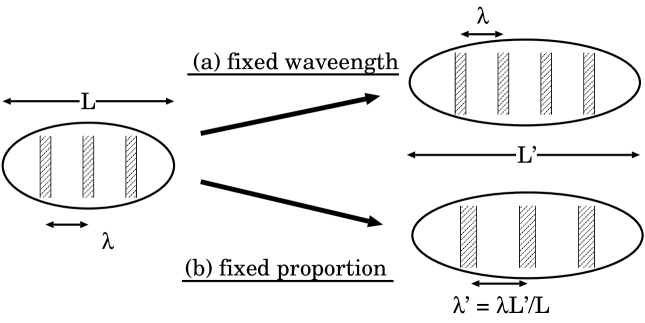
Figure 1: Ishihara and Kaneko

Figure 2: Ishihara and Kaneko

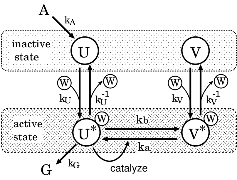
Figure 3: Ishihara and Kaneko

Figure 4: Ishihara and Kaneko

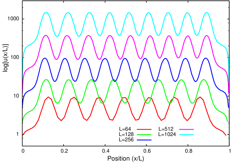
Figure 5: Ishihara and Kaneko

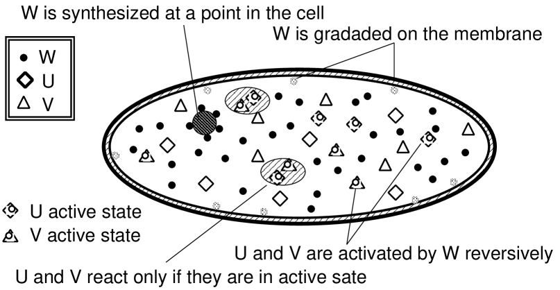
Figure 6: Ishihara and Kaneko

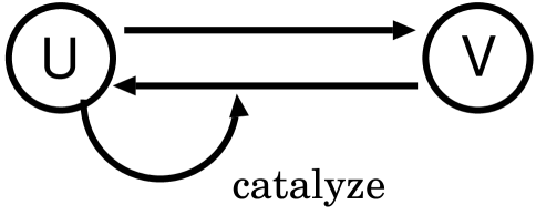
Figure 7: Ishihara and Kaneko

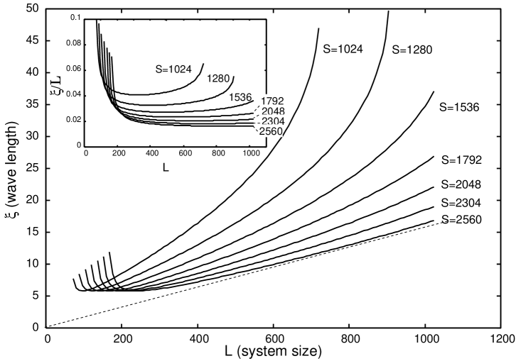
Figure 8: Ishihara and Kaneko

Figure 9: Ishihara and Kaneko

Figure 10: Ishihara and Kaneko