Biological remodelling: Stationary energy, configurational change, internal variables and dissipation

Abstract

Remodelling is defined as an evolution of microstructure or variations in the configuration of the underlying manifold. The manner in which a biological tissue and its subsystems remodel their structure is treated in a continuum mechanical setting. While some examples of remodelling are conveniently modelled as evolution of the reference configuration (Case I), others are more suited to an internal variable description (Case II). In this paper we explore the applicability of stationary energy states to remodelled systems. A variational treatment is introduced by assuming that stationary energy states are attained by changes in microstructure via one of the two mechanisms—Cases I and II. An example is presented to illustrate each case. The example illustrating Case II is further studied in the context of the thermodynamic dissipation inequality.

1 Introduction and background

The development of a biological tissue and its subsystems consists of the distinct processes of morphogenesis, growth and remodelling, a classification suggested by Taber (1995). For preciseness of mathematical formulation we have previously defined and treated growth as consisting of only addition or depletion of mass through processes of transport and reaction, possibly coupled with mechanics (Garikipati et al., 2004). We define remodelling as microstructural changes within the biological structure at constant mass. While remodelling and growth occur simultaneously and in a coupled fashion in biological tissues, they can be treated as separate processes for modelling purposes. Furthermore, in certain situations, addition and depletion remain in balance, maintaining constant mass. This is referred to as homeostasis, during which remodelling can occur.

There is, in fact, experimental evidence for a strict separation between remodelling and growth in soft tissue: (i) Stopak and Harris (1982) described the orientation of collagen fibrils due to the forces exerted on them by the fibroblasts (tendon cells) in a collagen gel. Growth processes of resorption of existing fibrils and production of new ones with the preferred orientation were not reported in their paper, suggesting that it was the mechanical action of fibroblasts alone that resulted in fibril orientation. In this example the fibril orientation can be viewed as the microstructural quantity undergoing an evolution in the absence of growth. Fibril reorientation driven by stress and occurring independently of growth was attained in our laboratory: A collagen gel was formed in a dish with polyethylene supports fixed to the base. When fibroblasts were added to the gel they exerted traction, thereby aligning the collagen fibrils. The orientation that was obtained corresponded to the axis defined by the supports. (ii) Another instance of microstructural change in collagen fibrils is their longitudinal and lateral fusion. Birk et al. (1995, 1997) reported an abrupt change in the length of embryonic chicken tendons from $\approx 40\;\mu$m to $\approx 120\;\mu$m, on the $17^{\mathrm{th}}$ day after fertilization. In this case, while growth obviously was taking place in the embryonic tendon, micrographs verified the abrupt change to be due to longitudinal (end-to-end) fusion of smaller fibrils. This time scale, over which fusion took place, is much smaller than the time scale of growth. We therefore propose that, in a mathematical treatment, it is appropriate to view this remodelling process as taking place in the absence of growth.

In contrast to these examples in soft tissue stands the case of bone, wherein the macroscopic process that is usually labelled “remodelling” takes place by resorption of existing collagen fibrils and production of new fibrils with a preferred orientation. In this case, therefore, the finer scale processes do fit our definition of growth. For the sake of conceptual and mathematical clarity we will ignore all processes that require growth at any scales in this paper, and focus upon a continuum mechanical treatment of remodelling.

The literature in biomechanics and mathematical biology has a number of papers concerning “remodelling” (Cowin and Hegedus, 1976; Taber, 1995; Harrigan and Hamilton, 1993; Seliktar et al., 2000; Taber and Humphrey, 2001; Ambrosi and Mollica, 2002). Almost universally, however, these papers treat mass and density changes and the mechanics—characterized by internal stress—that is associated with them. Therefore, by our definition, they describe growth. An exception is Humphrey and Rajagopal (2002), in which the notion of a natural configuration is introduced. It bears some similarities with the treatment in Section 2 of this paper.

Another treatment, by Driessen et al. (2003), is specific to the evolution of fiber orientation within a tissue. However, there are at least two fundamental shortcomings in their model: (i) It is unable to distinguish between cubic orthotropy and isotropy, and (ii) it predicts that in a tissue that is undeformed from its reference state, the fiber orientations evolve until a tensorial variable representing their distribution reaches a particular value. We discuss their model and present a critique of both these features in Section 4.4.

The following is the organization of this paper: The mathematical treatment for cases that are best described by smooth configurational changes on the underlying manifold (Case I remodelling) is presented in Section 2. A one-dimensional example is presented in Section 3 to illustrate this formulation. The local reorientation of collagen fibrils, including our experiments and the treatment via internal variables is discussed in Section 4. Thermodynamic dissipation is discussed in Section 5. The paper concludes with a brief discussion in Section 6.

2 Case I remodelling: Microstructural changes that alter the reference configuration

Figure 1 depicts the kinematics associated with Case I remodelling. Material particles are labelled by $\mbox{\boldmath$X$}\in\mathbb{R}^{3}$ in the reference configuration, which is denoted by $\Omega_{0}\subset\mathbb{R}^{3}$. The material microstructure undergoes changes that can be described by a point-to-point vector map, $\mbox{\boldmath$\chi$}\mbox{\boldmath$\colon$}\Omega_{0}\times[0,T]\mapsto\mathbb{R}^{3}$, defined as $\mbox{\boldmath$\chi$}(\mbox{\boldmath$X$},t)\equiv\mbox{\boldmath$X$}+\mbox{\boldmath$\kappa$}(\mbox{\boldmath$X$},t)$. It carries the microstructure from the reference configuration to a remodelled configuration, $\Omega^{\ast}$, in which material points will also be labelled as $\mbox{\boldmath$X$}^{\ast}=\mbox{\boldmath$\chi$}$. Assuming $\mbox{\boldmath$\chi$}(\mbox{\boldmath$X$},t)$ to be smooth in $X$, its tangent map is $\mbox{\boldmath$K$}(\mbox{\boldmath$X$},t)=\partial\mbox{\boldmath$\chi$}/\partial\mbox{\boldmath$X$}$, leading to $\mbox{\boldmath$K$}={\bf 1}+\partial\mbox{\boldmath$\kappa$}/\partial\mbox{\boldmath$X$}$. In Case I remodelling, therefore, $K$ denotes a compatible change in configuration.

Distinct from $\chi$ is the point-to-point vector map $\mbox{\boldmath$\varphi$}^{\ast}\mbox{\boldmath$\colon$}\Omega^{\ast}\times[0,T]\mapsto\mathbb{R}^{3}$. It carries material points from $\Omega^{\ast}$ to the spatial configuration $\Omega$, and is the deformation relative to $\Omega^{\ast}$. The placement of material points in $\Omega$ is therefore $\mbox{\boldmath$x$}=\mbox{\boldmath$\varphi$}^{\ast}(\mbox{\boldmath$X$}^{\ast},t)$. The displacement, $\mbox{\boldmath$u$}^{\ast}$, satisfies $\mbox{\boldmath$\varphi$}^{\ast}(\mbox{\boldmath$X$}^{\ast},t)=\mbox{\boldmath$X$}^{\ast}+\mbox{\boldmath$u$}^{\ast}(\mbox{\boldmath$X$}^{\ast},t)$. The classical deformation gradient is $\mbox{\boldmath$F$}^{\ast}:=\partial\mbox{\boldmath$\varphi$}^{\ast}/\partial\mbox{\boldmath$X$}^{\ast}={\bf 1}+\partial\mbox{\boldmath$u$}^{\ast}/\partial\mbox{\boldmath$X$}^{\ast}$. In this initial treatment we do not consider any further decompositions of $\mbox{\boldmath$F$}^{\ast}$. The overall motion of a point is $\mbox{\boldmath$\varphi$}(\mbox{\boldmath$X$},t)=\mbox{\boldmath$\kappa$}(\mbox{\boldmath$X$},t)+\mbox{\boldmath$u$}^{\ast}(\mbox{\boldmath$X$}^{\ast},t)\circ\mbox{\boldmath$\chi$}(\mbox{\boldmath$X$},t)$, and the corresponding tangent map is $\mbox{\boldmath$F$}=\partial\mbox{\boldmath$\varphi$}/\partial\mbox{\boldmath$X$}$. It admits the multiplicative decomposition $\mbox{\boldmath$F$}=\mbox{\boldmath$F$}^{\ast}\mbox{\boldmath$K$}$.

\psfrag{A}{\small$\Omega_{0}$}\psfrag{B}{\small$\Omega^{\ast}$}\psfrag{C}{\small$\Omega$}\psfrag{D}{\small$\mbox{\boldmath$\varphi$}$}\psfrag{G}{\small$\mbox{\boldmath$\varphi$}^{\ast}$}\psfrag{E}{\small$\mbox{\boldmath$\chi$}$}\includegraphics[width=284.52756pt]{remodel2.eps}

Figure 1: The kinematics of Case I remodelling and deformation.

Remark 1: In applications, the microstructural motion, $\chi$, will be distinguished from the deformation, $\mbox{\boldmath$\varphi$}^{\ast}$, by either physical or mathematical considerations. For instance, in the example of Section 3, $\chi$ denotes the uncoiling of a long-chain molecule, while $\mbox{\boldmath$\varphi$}^{\ast}$ is the stretching of bonds. A mathematical decomposition can be motivated in other applications such as $\chi$ denoting fine scale motion of material particles, while $\mbox{\boldmath$\varphi$}^{\ast}$ denotes motion on coarser scales.

2.1 A variational formulation

We wish to explore the relevance of stationary energy states to remodelled biological systems. For this purpose the microstructural changes of the type outlined with examples from biology in Section 1 and discussed more mathematically in this section, are assumed to occur when the Gibbs free energy of the system attains a stationary state. Importantly, the stationary state of the biological system is not one of equilibrium. The latter class of states is dictated by thermodynamic dissipation (see de Groot and Mazur, 1984). The stationary energy states, on the other hand, can be identified via standard variational arguments. For this purpose we consider the following Gibbs free energy functional:

$$\Pi_{I}[\mbox{\boldmath$u$}^{\ast},\mbox{\boldmath$\kappa$}] = \int\limits_{\Omega^{\ast}}\hat{\psi}^{\ast}(\mbox{\boldmath$F$}^{\ast},\mbox{\boldmath$K$},\mbox{\boldmath$X$}^{\ast})\mathrm{d}V^{\ast}$$ (1)

$$-\int\limits_{\Omega^{\ast}}\mbox{\boldmath$f$}^{\ast}\mbox{\boldmath$\cdot$}(\mbox{\boldmath$u$}^{\ast}+\mbox{\boldmath$\kappa$})\mathrm{d}V^{\ast}-\int\limits_{\partial\Omega^{\ast}_{t}}\bar{\mbox{\boldmath$t$}}^{\ast}\mbox{\boldmath$\cdot$}(\mbox{\boldmath$u$}^{\ast}+\mbox{\boldmath$\kappa$})\mathrm{d}A^{\ast},$$

where $\psi^{\ast}=\hat{\psi}^{\ast}(\mbox{\boldmath$F$}^{\ast},\mbox{\boldmath$K$},\mbox{\boldmath$X$}^{\ast})$ is the Helmholtz free energy density function, defined per unit volume in the remodelled configuration. Observe that $\psi^{\ast}$ is assumed to depend upon $K$ in addition to the usual dependence on $\mbox{\boldmath$F$}^{\ast}$. Material heterogeneity is allowed, and is represented by the dependence of $\hat{\psi}^{\ast}$ on $\mbox{\boldmath$X$}^{\ast}$. The body force per unit volume in $\Omega^{\ast}$ is $\mbox{\boldmath$f$}^{\ast}$, and the applied traction per unit area of the surface subset, $\partial\Omega^{\ast}_{t}\subset\partial\Omega^{\ast}$, is $\bar{\mbox{\boldmath$t$}}^{\ast}$. We allow for displacement boundary conditions, $\mbox{\boldmath$u$}^{\ast}=\mbox{\boldmath$g$}^{\ast}$, and vanishing microstructural change, $\mbox{\boldmath$\kappa$}={\bf 0}$ on $\partial\Omega^{\ast}_{u}=\partial\Omega^{\ast}\backslash\partial\Omega^{\ast}_{t}$. Since the total motion of a material point is $\mbox{\boldmath$\kappa$}+\mbox{\boldmath$u$}^{\ast}$, the potential energy of the external loads is as expressed by the second and third terms in (1).

2.1.1 Euler-Lagrange equation: Quasistatic balance of linear momentum

The functional (1) yields one set of Euler-Lagrange equations when stationarity of $\Pi_{I}$ is imposed with respect to variations in $\mbox{\boldmath$u$}^{\ast}$. We first define $\mbox{\boldmath$u$}^{\ast}_{\varepsilon}:=\mbox{\boldmath$u$}^{\ast}+\varepsilon\delta\mbox{\boldmath$u$}^{\ast}$, at fixed $\kappa$, with $\delta\mbox{\boldmath$u$}^{\ast}\in\mathbb{R}^{3}$ and $\delta\mbox{\boldmath$u$}^{\ast}={\bf 0}$ on $\partial\Omega^{\ast}_{u}$. Then,

$$\frac{\mathrm{d}}{\mathrm{d}\varepsilon}\Pi_{I}[\mbox{\boldmath$u$}^{\ast}_{\varepsilon},\mbox{\boldmath$\kappa$}] = \frac{\mathrm{d}}{\mathrm{d}\varepsilon}\left(\int\limits_{\Omega^{\ast}}\hat{\psi}^{\ast}(\mbox{\boldmath$F$}^{\ast}_{\varepsilon},\mbox{\boldmath$K$},\mbox{\boldmath$X$}^{\ast})\mathrm{d}V^{\ast}-\int\limits_{\Omega^{\ast}}\mbox{\boldmath$f$}^{\ast}\mbox{\boldmath$\cdot$}(\mbox{\boldmath$u$}^{\ast}_{\varepsilon}+\mbox{\boldmath$\kappa$})\mathrm{d}V^{\ast}\right)$$

$$-\frac{\mathrm{d}}{\mathrm{d}\varepsilon}\int\limits_{\partial\Omega^{\ast}_{t}}\bar{\mbox{\boldmath$t$}}^{\ast}\mbox{\boldmath$\cdot$}(\mbox{\boldmath$u$}^{\ast}_{\varepsilon}+\mbox{\boldmath$\kappa$})\mathrm{d}A^{\ast}.$$

Differentiating under the integrals, applying the chain rule, integrating by parts, and imposing stationarity via $(\mathrm{d}\Pi_{I}/\mathrm{d}\varepsilon)_{\varepsilon=0}=0$ gives

$$-\int\limits_{\Omega^{\ast}}\mathrm{Div}^{\ast}[\frac{\partial\psi^{\ast}}{\partial\mbox{\boldmath$F$}^{\ast}}]\mbox{\boldmath$\cdot$}\delta\mbox{\boldmath$u$}^{\ast}\mathrm{d}V^{\ast}-\int\limits_{\Omega^{\ast}}\mbox{\boldmath$f$}^{\ast}\mbox{\boldmath$\cdot$}\delta\mbox{\boldmath$u$}^{\ast}\mathrm{d}V^{\ast}$$

$$\qquad\qquad+\int\limits_{\partial\Omega^{\ast}_{t}}\left(\frac{\partial\psi^{\ast}}{\partial\mbox{\boldmath$F$}^{\ast}}\mbox{\boldmath$N$}^{\ast}\right)\mbox{\boldmath$\cdot$}\delta\mbox{\boldmath$u$}^{\ast}\mathrm{d}A^{\ast}-\int\limits_{\partial\Omega^{\ast}_{t}}\bar{\mbox{\boldmath$t$}}^{\ast}\mbox{\boldmath$\cdot$}\delta\mbox{\boldmath$u$}^{\ast}\mathrm{d}A^{\ast}=0.$$ (2)

Introducing $\mbox{\boldmath$P$}^{\ast}=\partial\psi^{\ast}/\partial\mbox{\boldmath$F$}^{\ast}$, the arbitrariness of $\delta\mbox{\boldmath$u$}^{\ast}\in\mathbb{R}^{3}$ and the standard localization argument yield the Euler-Lagrange equation

$$\mathrm{Div}^{\ast}\mbox{\boldmath$P$}^{\ast}+\mbox{\boldmath$f$}^{\ast}={\bf 0}\;\mathrm{in}\;\Omega^{\ast},$$ (3)

the following boundary condition and constitutive relation

$$\mbox{\boldmath$P$}^{\ast}\mbox{\boldmath$N$}^{\ast}=\bar{\mbox{\boldmath$t$}}^{\ast}\;\mathrm{on}\;\partial\Omega^{\ast}_{t},\quad\mbox{\boldmath$P$}^{\ast}\equiv\frac{\partial\psi^{\ast}}{\partial\mbox{\boldmath$F$}^{\ast}}.$$ (4)

Of these equations, (3) is recognized as the quasistatic balance of linear momentum in $\Omega^{\ast}$, and (4)₁ as the corresponding traction boundary condition. Observe that, as defined in (4)₂, $\mbox{\boldmath$P$}^{\ast}$ is the first Piola-Kirchhoff stress, which is conjugate to $\mbox{\boldmath$F$}^{\ast}$ with $\psi^{\ast}$ as the relevant strain energy density function.

2.1.2 Euler-Lagrange equation: Stationarity with respect to microstructural change

The class of variations now considered is given by

$$\mbox{\boldmath$\kappa$}_{\varepsilon}:=\mbox{\boldmath$\kappa$}+\varepsilon\delta\mbox{\boldmath$\kappa$},\quad\mbox{at fixed}\;\mbox{\boldmath$u$}^{\ast},\;\mbox{with}\,\delta\mbox{\boldmath$\kappa$}={\bf 0}\;\mbox{on}\,\partial\Omega^{\ast}_{u}.$$ (5)

Proceeding as in Section 2.1.1:

$$\frac{\mathrm{d}}{\mathrm{d}\varepsilon}\Pi_{I}[\mbox{\boldmath$u$}^{\ast},\mbox{\boldmath$\kappa$}_{\varepsilon}]=\frac{\mathrm{d}}{\mathrm{d}\varepsilon}\left(\int\limits_{\Omega^{\ast}}\hat{\psi}^{\ast}(\mbox{\boldmath$F$}^{\ast}_{\varepsilon},\mbox{\boldmath$K$}_{\varepsilon},\mbox{\boldmath$X$}^{\ast}_{\varepsilon})\mathrm{d}V^{\ast}-\int\limits_{\Omega^{\ast}}\mbox{\boldmath$f$}^{\ast}\mbox{\boldmath$\cdot$}(\mbox{\boldmath$u$}^{\ast}+\mbox{\boldmath$\kappa$}_{\varepsilon})\mathrm{d}V^{\ast}\right)\qquad$$

$$-\frac{\mathrm{d}}{\mathrm{d}\varepsilon}\int\limits_{\partial\Omega^{\ast}_{t}}\bar{\mbox{\boldmath$t$}}^{\ast}\mbox{\boldmath$\cdot$}(\mbox{\boldmath$u$}^{\ast}+\mbox{\boldmath$\kappa$}_{\varepsilon})\mathrm{d}A^{\ast},$$

where the following relations hold:

$$\mbox{\boldmath$F$}^{\ast}_{\varepsilon}=\mbox{\boldmath$F$}_{\varepsilon}\mbox{\boldmath$K$}_{\varepsilon}^{-1},\;\;\;\mbox{\boldmath$X$}^{\ast}_{\varepsilon}=\mbox{\boldmath$X$}+\mbox{\boldmath$\kappa$}_{\varepsilon},\;\;\;\mbox{\boldmath$K$}_{\varepsilon}={\bf 1}+\partial\mbox{\boldmath$\kappa$}/\partial\mbox{\boldmath$X$}+\varepsilon\frac{\partial\delta\mbox{\boldmath$\kappa$}}{\partial\mbox{\boldmath$X$}}.$$ (6)

Standard, if lengthy, manipulations (see Appendix A) then lead to the following set of equations governing the stationary energy state in which the configurational variables take on the values $\mbox{\boldmath$\kappa$}=\mbox{\boldmath$\kappa$}^{\mathrm{s}}$ and $\mbox{\boldmath$K$}=\mbox{\boldmath$K$}^{\mathrm{s}}$.

$$-\mathrm{Div}^{\ast}\left(\psi^{\ast}{\bf 1}-\mbox{\boldmath$F$}^{\ast^{\mathrm{T}}}\mbox{\boldmath$P$}^{\ast}+\mbox{\boldmath$\Sigma$}^{\ast}\right)+\frac{\partial\psi^{\ast}}{\partial\mbox{\boldmath$X$}^{\ast}} ={\bf 0} \;\mathrm{in}\quad\Omega^{\ast}$$ (7)

$$\left(\psi^{\ast}{\bf 1}-\mbox{\boldmath$F$}^{\ast^{\mathrm{T}}}\mbox{\boldmath$P$}^{\ast}+\mbox{\boldmath$\Sigma$}^{\ast}\right)\mbox{\boldmath$N$}^{\ast} ={\bf 0} \;\mathrm{on}\quad\partial\Omega^{\ast}_{t},$$ (8)

$$\mbox{where}\quad\mbox{\boldmath$\Sigma$}^{\ast} \equiv\frac{\partial\psi^{\ast}}{\partial\mbox{\boldmath$K$}}\mbox{\boldmath$K$}^{\mathrm{T}} \;\mathrm{in}\quad\Omega^{\ast}$$ (9)

Observe that the Eshelby stress $\psi^{\ast}{\bf 1}-\mbox{\boldmath$F$}^{\ast^{\mathrm{T}}}\mbox{\boldmath$P$}^{\ast}$ makes its appearance. Hereafter, it will be denoted by ${\mathcal{E}}$. The quantity $\mbox{\boldmath$\Sigma$}^{\ast}$ is a thermodynamic driving force defined in (9) as the change in Helmholtz free energy density corresponding to a change in the tangent map of the microstructural configuration. It is stress-like in its physical dimensions and is a second-order tensor. For this reason we refer to it as a non-Eshelbian configurational stress. The boundary condition in (8) is simply a restriction on the normal component of this thermodynamic driving term.

2.1.3 Stationarity with simultaneous variation of $\mbox{\boldmath$u$}^{\ast}$ and $\kappa$

The procedure followed above is formal in the sense that the independent imposition of variations has been assumed: $\mbox{\boldmath$u$}^{\ast}_{\varepsilon}=\mbox{\boldmath$u$}^{\ast}+\varepsilon\delta\mbox{\boldmath$u$}^{\ast}$ for $\delta\mbox{\boldmath$\kappa$}={\bf 0}$, and $\mbox{\boldmath$\kappa$}_{\varepsilon}=\mbox{\boldmath$\kappa$}+\varepsilon\delta\mbox{\boldmath$\kappa$}$ for $\delta\mbox{\boldmath$u$}^{\ast}={\bf 0}$. Physically, this may not be possible due to the interaction of deformation and configurational changes. Stationarity of the Gibbs free energy under simultaneous variation of its arguments is obtained by requiring

$$\frac{\mathrm{d}}{\mathrm{d}\varepsilon}\Pi_{I}[\mbox{\boldmath$u$}^{\ast}_{\varepsilon},\mbox{\boldmath$\kappa$}_{\varepsilon}]\big{|}_{\varepsilon=0}=0.$$

On carrying out this calculation as in Sections 2.1.1, 2.1.2 and Appendix A it can be shown that stationarity requires the following condition:

$$\int\limits_{\Omega^{\ast}}\left(\left(\mathrm{Div}^{\ast}\mbox{\boldmath$P$}^{\ast}+\mbox{\boldmath$f$}^{\ast}\right)\mbox{\boldmath$\cdot$}\delta\mbox{\boldmath$u$}^{\ast}+\left(\mathrm{Div}^{\ast}\left(\mbox{\boldmath{${\mathcal{E}}$}}+\mbox{\boldmath$\Sigma$}^{\ast}\right)+\frac{\partial\psi^{\ast}}{\partial\mbox{\boldmath$X$}^{\ast}}\right)\mbox{\boldmath$\cdot$}\delta\mbox{\boldmath$\kappa$}\right)\mathrm{d}V^{\ast}$$

$$\hskip 42.67912pt-\int\limits_{\partial\Omega^{\ast}_{t}}\left(\left(\mbox{\boldmath$P$}^{\ast}\mbox{\boldmath$N$}^{\ast}-\bar{\mbox{\boldmath$t$}}^{\ast}\right)\mbox{\boldmath$\cdot$}\delta\mbox{\boldmath$u$}^{\ast}+\left(\left(\mbox{\boldmath{${\mathcal{E}}$}}+\mbox{\boldmath$\Sigma$}\right)\mbox{\boldmath$N$}^{\ast}\right)\mbox{\boldmath$\cdot$}\delta\mbox{\boldmath$\kappa$}\right)\mathrm{d}A^{\ast}=0,$$ (10)

where the notation introduced above for the Eshelby stress and the non-Eshelbian configurational stress has been used. Clearly (3–4) and (7–9) ensure satisfaction of (10), and are therefore sufficient conditions for stationarity.

3 An example of Case I remodelling: Configurational change of a long chain molecule

In this section we employ an established statistical mechanical example of configurational changes of long chain molecules in order to illuminate the mathematical formulation of Section 2. In addition to the interest in this example from the standpoint of this paper we point out that configurational changes are of central importance to the chemical activity of long chain molecules.

Consider a long-chain molecule, say a protein, that can exist in a highly coiled state. Let its contour length be $L$. In the reference state, $\Omega_{0}$, the end-to-end lengths of the coiled and the relatively straight domains are in the ratio $\xi\;\colon\;1-\xi$, and the end-to-end length of the molecule is $r_{0}$ (Figure 2). An entropic elasticity is associated with uncoiling of the molecule. Let $\kappa$ be the change in end-to-end length from the reference state due to uncoiling; it is a measure of changes in the number of configurations available (entropy). The corresponding contribution to the Gibbs free energy function is specified by the worm-like chain (WLC) model (Kratky and Porod, 1949). A stiffness, $\mu$, with physical dimensions of energy is associated with bond stretching. The increase in length due to bond stretching is $u^{\ast}$. The square of the ratio of this quantity and the length of the molecule, $\kappa+r_{0}$, determines the energy stored in bonds. The enthalpic elasticity is due to this mechanism. The molecule is subjected to an externally-applied axial tensile force, $T$.

\psfrag{T}{\tiny$T$}\psfrag{O}{\tiny$\frac{r_{0}}{2}(1-\xi)$}\psfrag{X}{\tiny$r_{0}\xi$}\psfrag{K}{\tiny$\kappa$}\psfrag{U}{\tiny$u^{\ast}$}\psfrag{P}{}\psfrag{Q}{}\psfrag{L}{\tiny$\kappa+r_{0}$}\includegraphics[width=341.43306pt]{chain_molecule.eps}

Figure 2: A long chain molecule that can undergo configurational changes and bond stretching due to an external axial load. For ease of visualization the figure depicts bond stretching only in the uncoiled, straight regions.

The one-dimensional tangent map of the local configurational change, averaged over the entire molecule, is $K=1+\kappa/r_{0}$. It carries the molecule to its remodelled configuration, $\Omega^{\ast}$. The one-dimensional deformation gradient relative to $\Omega^{\ast}$ is $F^{\ast}=1+u^{\ast}/(\kappa+r_{0})$, also averaged over the molecule. It carries the molecule to its current configuration, $\Omega$, in which it has undergone a configurational change and bond stretching.

We will examine the response of the molecule to the axial force. In this case, the Gibbs free energy is

$$\Pi_{I}[u^{\ast},\kappa] = \frac{1}{2}\mu\left(\frac{u^{\ast}}{\kappa+r_{0}}\right)^{2}$$ (11)

$$+\frac{k_{B}\theta}{A}\left(\frac{(\kappa+r_{0})^{2}}{2L}+\frac{L}{4(1-(\kappa+r_{0})/L)}-\frac{\kappa+r_{0}}{4}\right)$$

$$-T(u^{\ast}+\kappa),$$

where the first term on the right hand-side is the Helmholtz free energy from elastic stretching. The second term is the entropic contribution from the WLC model, after Marko and Siggia (1995), with $k_{B}$ being the Boltzmann constant and $\theta$ being the temperature. The persistence length is $A$ and is defined as the ratio of bending stiffness to the thermal energy. It is also the distance along the molecule’s contour over which the correlation between tangent vectors falls to $e^{-1}$. See Landau and Lifshitz (1951) for the statistical mechanics behind these aspects of the model. The third term in (11) is the potential of the external force.

Proceeding as in Section 2 we first seek stationarity with respect to variations in $u^{\ast}$:

$$\frac{\mathrm{d}}{\mathrm{d}\varepsilon}\Pi_{I}[u^{\ast}_{\varepsilon},\kappa]\Big{|}_{\varepsilon=0}=\mu\frac{u^{\ast}}{(\kappa+r_{0})^{2}}-T=0.$$ (12)

For this example, in the absence of a body force (3) reduces to the trivial requirement that the axial force be constant along the molecule. Equation (12) is the traction boundary condition (4)₁ for the present case. Solving, we get

$${u^{\ast}}^{\mathrm{s}}=\frac{T}{\mu}(\kappa+r_{0})^{2},$$ (13)

where superscript $(\bullet)^{s}$ denotes a quantity with respect to which the system is in a stationary state.

Next, considering variations with respect to $\kappa$ and imposing stationarity gives

$$\frac{\mathrm{d}}{\mathrm{d}\varepsilon}\Pi_{I}[u^{\ast},\kappa_{\varepsilon}]\Big{|}_{\varepsilon=0} = -\mu\frac{{u^{\ast}}^{2}}{(\kappa+r_{0})^{3}}-T$$ (14)

$$+\frac{k_{B}\theta}{A}\left(\frac{\kappa+r_{0}}{L}+\frac{1}{4\left(1-(\kappa+r_{0})/L\right)^{2}}-\frac{1}{4}\right)$$

$$= 0.$$

In this case the differential equation (7) is trivially satisfied since the forces corresponding to the stresses ${\mathcal{E}}$ and $\mbox{\boldmath$\Sigma$}^{\ast}$ are constant along the molecule.

The first term in the second member of (14) arises due to the variation of $F^{\ast}$ with $\kappa$. It represents the effect of variation in the underlying manifold, $\Omega^{\ast}$, due to configurational changes. On comparison with (38) and (39), and following the derivation in Appendix A it is clear that this term is the reduced version of the Eshelby stress for the present one-dimensional setting. The third term of the second member of (14) arises due to the variation of the WLC term with $\kappa$. It represents the non-Eshelbian stress reduced to this setting as is confirmed by comparison with the development in Appendix A.

The reduced version of the boundary condition (8) is obtained on substituting the stationary solution (13) for $u^{\ast}$ in Equation (14). (In effect, this is the substitution referred to at the end of Appendix A.):

$$-\frac{T^{2}}{\mu}(\kappa+r_{0})+\frac{k_{B}\theta}{A}\left(\frac{\kappa+r_{0}}{L}+\frac{1}{4\left(1-(\kappa+r_{0})/L\right)^{2}}-\frac{1}{4}\right)-T=0.$$ (15)

Solutions to (15), denoted by $\kappa^{\mathrm{s}}$, can be obtained in closed-form since it is a cubic equation. In order to illustrate the nature of the solution we have plotted the left hand-side of (15) against $\kappa$ in Figure 3 with the numerical values of parameters in Table 1. The plot is restricted to the interval $0\leq\kappa<L-r_{0}$, since uncoiling is of interest, and (11) is non-physical for $\kappa\geq L-r_{0}$.

Table 1: Parameters used in the Gibbs free energy of the long chain molecule

P   arameter	Value	Units	Notes
$\xi$	$1$	-	-
$\theta$	$300$	K	-
$A$	$14.5$	nm	Collagen monomer molecule (Sun et al., 2002)
$r_{0}$	$120$	nm	-
$L$	$309$	nm	Collagen monomer molecule (Sun et al., 2002)
$\mu$	$2.951\times 10^{-7}$	J	Stiff bonds
$T$	$10$	pN	Force applied in Sun et al. (2002)

\psfrag{X}{\small$\kappa$ (nm)}\psfrag{Y}{\small$D\Pi_{I}$ (N)}\includegraphics[angle={0},width=227.62204pt]{energy4.eps}

Figure 3: Variation of $D\Pi_{I}=(\mathrm{d}\Pi_{I}/\mathrm{d}\varepsilon)_{\varepsilon=0}$ with respect to $\kappa$.

The variation in free energy $D\Pi_{I}=(\mathrm{d}\Pi_{I}/\mathrm{d}\varepsilon)_{\varepsilon=0}$ is negative over most of the $\kappa$-interval and passes through zero at $\kappa^{\mathrm{s}}=162.642$ nm. This is the length increase due to uncoiling when the molecule is in the stationary energy state. Corresponding to this value is the bond stretch, ${u^{\ast}}^{\mathrm{s}}=3\times 10^{-9}$ nm. The molecule is very stiff—almost rigid—to bond stretching. Also observe that the stress-stretch response determined by the WLC model locks as $\kappa^{\mathrm{s}}\to L-r_{0}$ from below ($\kappa^{\mathrm{s}}\to 189$ nm); i.e., as the uncoiled length approaches the contour length.

Remark 2: The uncoiling, represented by $\kappa$, takes place under an axial force and its effect on the free energy is treated via a model of entropic elasticity. It therefore follows that the entropy of the molecule is reversibly changed by application and removal of a force.

4 Case II remodelling: Microstructural changes represented by internal variables

While microstructural changes always imply an evolution of the reference configuration, a simpler description may be possible than the general one developed in Section 2. Such an instance is illustrated by the example of collagen fibril reorientation under mechanical load: The reorientation of a fibril does modify the reference configuration since the underlying microstructure changes, and hence the general formulation of Section 2 remains applicable. However, the physics of the process admits a simpler model that requires only the introduction of a rotation tensor as an internal variable and is discussed below. We begin with the biological basis and include a description of our experiments.

4.1 Collagen fibril alignment in gels by cell traction

Collagen is the most widely-present protein in the human body. It exists in many forms of which, to fix ideas, we will consider type I collagen. It has a fibrillar structure and is the main form of collagen in tendons. The fundamental unit is the triple helical collagen molecule that is assembled from three single chain molecular strands. The triple helix has been reported to be between 300 to 360 nm in length and 1.5 nm in diameter. The triple helices further assemble into collagen fibrils of varying lengths (the range of 20–140 $\mu$m has been reported) and 10–300 nm in diameter. The fibrils assemble into fibers that can range up to millimeters in length. The collagen fibrils are surrounded by a dense network of proteoglycan (PG) molecules, which, at one end, associate with the collagen fibrils. They form a hydrated gel that contains most of the fluid phase of the extracellular matrix. Other extracellular matrix proteins are also found in the gel. The interested reader is directed to Alberts et al. (2002, chap. 19) and references therein for details.

Stopak and Harris (1982) have described the reorientation of collagen fibrils due to cell traction in gels. In their experiments, cell-bearing tissue explants were embedded in collagen gels. Cells were found to migrate outward from the explant, and, by applying traction, to induce a preferred alignment of the collagen network. Specifically, collagen fibrils were found to align either between a pair of explants, or an explant and a fixed, effectively rigid, support. In a three-dimensional environment, such as a collagen gel, the fibroblasts themselves align along directions of maximum principal tensile stress in the matrix (Balaban et al., 2001). In vitro (and probably in vivo also), the stress is often imposed by fibroblast traction on the matrix. In other in vitro studies an externally-applied traction has resulted in fibroblast alignment with the maximum principal tensile stress direction.

Fibroblasts attain alignment by attaching themselves to the matrix (usually the collagen fibrils) by “three-dimensional adhesion points”. Complex signalling pathways and chemical cascades are involved in the formation of these adhesion points (Cukierman et al., 2001). The actual attachment to the matrix is mediated by receptors called integrins that pass through the cell membrane and are attached to the intracellular actin network at the opposite end from the adhesion point. See Geiger et al. (2001); Mitra et al. (2005). A tensile stress develops in the actin network, the cell’s interinsic contractile apparatus, associated with stretching of the fibroblast between multiple adhesion points in the extra-cellular matrix. The stress in the actin network thus enables the fibroblast to apply traction to the matrix in a direction now determined by the alignment of adhesion points (Balaban et al., 2001). This traction induces a marked reorientation among the fibrils in a network with an initially random orientation distribution. The fibrils align with the maximum principal tensile stress direction in the matrix. There now exists general agreement that these mutual interactions between stress in the matrix, fibroblast alignment and stress in the actin network are responsible for the collagen fibril reorientation described in papers such as Stopak and Harris (1982).

4.2 Experimental study

In order to assess the role of fibroblasts in the alignment of collagen fibrils we carried out a set of simple collagen gel contraction experiments (that we have already alluded to in Section 1).

Three experimental configurations were considered. In the first, a cell-collagen solution was delivered over porous polyethylene posts spaced 6 mm apart (Figure 4). Over 12 hours, the cell-seeded gel contracted to form a linear structure stretched between the supporting posts. The contraction of the cell-collagen gel was observed (at ambient temperature 22^∘C) between crossed polarizing lenses mounted on an inverted microscope for 12–15 hours under 40$\times$ magnification using an attached digital camera. An observed increase in transmitted light through the polarizing filters over the recording period indicated a significant microstructural reorganization in addition to macroscopic changes in gel shape. The gel became birefringent due to alignment of collagen fibrils along the axis of the posts. In a second experiment, a nearly identical procedure was followed but without the addition of the constraining posts to the dish. While this gel contracted to half its original diameter overnight, the lack of constraints resulted in an isotropic contraction, no observable alignment of fibrils, and therefore no birefringence (data not shown). Finally, a third gel plated without cells was found to neither contract nor yield a birefringent species. Taking these results together, one can (reasonably) conclude that the alignment requires both traction-providing cells (i.e., fibroblasts) as well as fixed displacement constraints so that the stress field applied by the cells to the matrix is anisotropic and induces the reorientation of fibrils.

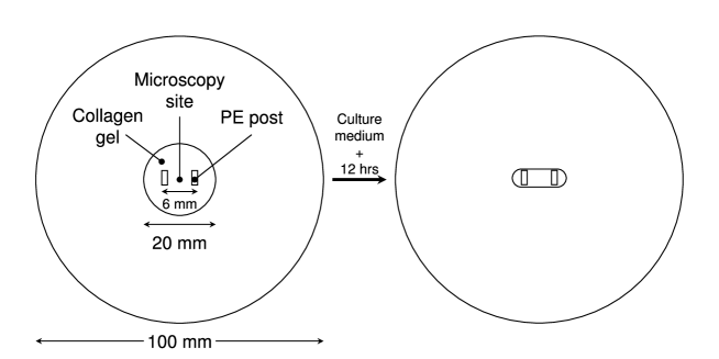
Figure 4: Schematic figure of the experimental setup for collagen gel formation and fibril alignment by cell traction.

4.3 Modelling assumptions leading to Case II

We make the following modelling assumptions on the alignment of fibrils by cell traction in a collagen gel:

1. We restrict ourselves to situations in which there is a uniform distribution of fibroblasts and fibrils in the gel. The typical linear dimension of a fibroblast is 25 $\mu$m. Therefore, at a macroscopic scale, each point in the gel has available the microstructural mechanisms required for collagen fibril reorientation.

2. Since the fibroblasts and fibrils are uniformly distributed, cell traction does not result in translation of the center of mass of the collagen fibril network within an infinitesimal neighborhood of a point. Therefore, the only effect of fibroblast traction on the fibrils is to change their alignment at a continuum point.

3. A consequence of Assumption 2 is that the fluid surrounding the collagen fibrils in the gel does not undergo a translation of its center of mass due to fibroblast traction.

4. There is no loss of contact between the fibrils and the surrounding fluid in the gel due to fibril realignment; i.e., local compatibility is maintained.

Reverting to Equation (1) we let the motion of material points induced by fibril rotation be denoted by $\kappa$. It follows from Assumptions 2 and 3 that the work done by forces $\mbox{\boldmath$f$}^{\ast}$ and $\bar{\mbox{\boldmath$t$}}^{\ast}$ on $\kappa$ vanishes in (1) .

At the macroscopic scale, we develop an internal variable description of the reorientation of the microscopic fibrils. In contrast to Case I remodelling (Section 2) we do not undertake a detailed consideration of the changes in reference configuration brought about by variation of this internal variable. The Gibbs free energy will depend on the internal variable for fibril reorientation since it determines pointwise anisotropy of the extracellular matrix. If the tangent to a fibril has an initial orientation given by the unit vector field $\mbox{\boldmath$M$}_{0}(\mbox{\boldmath$X$})\in\Omega_{0}$, then $\mbox{\boldmath$M$}^{\ast}(\mbox{\boldmath$X$},t)=\mbox{\boldmath$Q$}(\mbox{\boldmath$X$},t)\mbox{\boldmath$M$}_{0}(\mbox{\boldmath$X$})$ is its remodelled orientation at time $t$, where $\mbox{\boldmath$Q$}(\mbox{\boldmath$X$},t)\in SO(3)$, a rotation tensor, is the internal variable. We write the Helmholtz free energy density with respect to $\Omega_{0}$ as $\hat{\psi}(\mbox{\boldmath$F$},\mbox{\boldmath$Q$},\mbox{\boldmath$X$})$. Note that $\hat{\psi}$ is defined with respect to the reference configuration, changes in which we will ignore in Case II remodelling.

The Gibbs free energy functional is parametrized by the displacement $u$, now defined on $\Omega_{0}$, and $Q$. Reflecting the assumptions made above and the arguments following from them, Equation (1) reduces to

$$\Pi_{II}[\mbox{\boldmath$u$},\mbox{\boldmath$Q$}]=\int\limits_{\Omega_{0}}\hat{\psi}(\mbox{\boldmath$F$},\mbox{\boldmath$Q$},\mbox{\boldmath$X$})\mathrm{d}V-\int\limits_{\Omega_{0}}\mbox{\boldmath$f$}\mbox{\boldmath$\cdot$}\mbox{\boldmath$u$}\mathrm{d}V-\int\limits_{\partial\Omega_{0t}}\bar{\mbox{\boldmath$t$}}\mbox{\boldmath$\cdot$}\mbox{\boldmath$u$}\mathrm{d}A.$$ (16)

Note that the integrals are defined on $\Omega_{0}$. The body force and traction vectors are $f$ and $\bar{\mbox{\boldmath$t$}}$, respectively, defined per unit volume in $\Omega_{0}$ and per unit surface area on $\partial\Omega_{0}$. We now consider variations on $Q$, recalling that $SO(3)$ is a Lie group whose Lie algebra consists of real, skew-symmetric matrices. This Lie algebra is denoted by $\mathrm{Skw}(3)$ for the case wherein $Q$ acts on vectors in $\mathbb{R}^{3}$ (see any standard textbook on manifold analysis, for instance, Choquet-Bruhat et al. (1982)). The admissible variations on $Q$ are therefore of the form

$$\mbox{\boldmath$Q$}_{\varepsilon}=\mbox{\boldmath$Q$}+\delta\mbox{\boldmath$Q$},\;\;\mathrm{where}\;\delta\mbox{\boldmath$Q$}=\mbox{\boldmath$W$}\mbox{\boldmath$Q$}\,\forall\,\mbox{\boldmath$W$}\in\mathrm{Skw}(3).$$ (17)

This leads to the following variation on $\Pi_{II}$:

$$\frac{\mathrm{d}}{\mathrm{d}\varepsilon}\Pi_{II}[\mbox{\boldmath$u$},\mbox{\boldmath$Q$}_{\varepsilon}]\big{|}_{\varepsilon=0}=$$

$$\qquad\qquad\frac{\mathrm{d}}{\mathrm{d}\varepsilon}\left(\int\limits_{\Omega}\hat{\psi}(\mbox{\boldmath$F$},\mbox{\boldmath$Q$}_{\varepsilon},\mbox{\boldmath$X$})\mathrm{d}V-\int\limits_{\Omega}\mbox{\boldmath$f$}\mbox{\boldmath$\cdot$}\mbox{\boldmath$u$}\mathrm{d}V-\int\limits_{\partial\Omega_{t}}\bar{\mbox{\boldmath$t$}}\mbox{\boldmath$\cdot$}\mbox{\boldmath$u$}\mathrm{d}A\right)\Big{|}_{\varepsilon=0}.$$ (18)

Imposing stationarity, invoking the localization argument and applying (17) this reduces in a straightforward manner to

$$\frac{\partial\psi}{\partial\mbox{\boldmath$Q$}}\mbox{\boldmath$\colon$}\mbox{\boldmath$W$}\mbox{\boldmath$Q$}=0,\;\;\forall\;\mbox{\boldmath$W$}\in\mathrm{Skw}(3),$$ (19)

a relation also obtained by Vianello (1996), albeit without beginning from the integral form. As a final step this result for a stationary state can be rewritten as

$$\frac{\partial\psi}{\partial\mbox{\boldmath$Q$}}\mbox{\boldmath$Q$}^{\mathrm{T}}\Big{|}_{\mbox{\boldmath$Q$}=\mbox{\boldmath$Q$}^{\mathrm{s}}}\mbox{\boldmath$\colon$}\mbox{\boldmath$W$}=0,\;\;\forall\;\mbox{\boldmath$W$}\in\mathrm{Skw}(3).$$ (20)

4.3.1 Example: Collagen fibril reorientation in a gel using a continuum strain energy function

The WLC model (11) is extended to a continuum strain energy function for the system consisting of the gel, collagen fibrils and fibroblasts. This is achieved by introduction of the fibril number density, $N$, and addition of a repulsive term to enforce a vanishing stress at unit stretch and a bulk compressibility term for the gel:

$$\hat{\psi}(\mbox{\boldmath$F$},\mbox{\boldmath$Q$},\mbox{\boldmath$X$}) = \frac{Nk_{B}\theta}{4A}\left(\frac{2r^{2}}{L}+\frac{L}{1-r/L}-r\right)$$ (21)

$$\underbrace{-\frac{Nk_{B}\theta}{4A}\left(\frac{1}{L}+\frac{1}{4r_{0}(1-\frac{r_{0}}{L})^{2}}-\frac{1}{4r_{0}}\right)\log(\lambda^{4r_{0}^{2}})}_{\mbox{repulsive term}}$$

$$\underbrace{+\frac{\gamma}{\beta}(J^{-2\beta}-1)+2\gamma{\bf 1}\mbox{\boldmath$\colon$}\mbox{\boldmath$E$}}_{\mbox{bulk compressibility}}.$$

The elastic stretch in the direction of the remodelled fibril is $\lambda$, and $\mbox{\boldmath$E$}=\frac{1}{2}(\mbox{\boldmath$F$}^{\mathrm{T}}\mbox{\boldmath$F$}-{\bf 1})$ is the Lagrange strain. The factors $\gamma$ and $\beta$ control bulk compressibility. The end-to-end length is given by

$$r=\sqrt{r_{0}^{2}\lambda^{2}},\quad\lambda=\sqrt{\mbox{\boldmath$M$}^{\ast}\mbox{\boldmath$\cdot$}\mbox{\boldmath$F$}^{\mathrm{T}}\mbox{\boldmath$F$}\mbox{\boldmath$M$}^{\ast}}.$$ (22)

Note that the end-to-end length is modified by the macroscopic deformation through (22). This is in contrast with the explicit inclusion of the change in molecular configuration, $\kappa$, in (11). The change in configuration considered in the present section is at the more macroscopic scale of fibril reorientation.

Consider a cylindrically-shaped collagen gel in which the collagen fibrils are all radially-oriented at time $t=0$. Adopting a cylindrical coordinate system, $\{\mbox{\boldmath$e$}_{R},\mbox{\boldmath$e$}_{\alpha},\mbox{\boldmath$e$}_{Z}\}$, we have $\mbox{\boldmath$M$}_{0}=\mbox{\boldmath$e$}_{R}$. The gel is loaded by imposing a deformation gradient: $\mbox{\boldmath$F$}=\lambda_{R}\mbox{\boldmath$e$}_{R}\otimes\mbox{\boldmath$e$}_{R}+\lambda_{\alpha}\mbox{\boldmath$e$}_{\alpha}\otimes\mbox{\boldmath$e$}_{\alpha}+\lambda_{Z}\mbox{\boldmath$e$}_{Z}\otimes\mbox{\boldmath$e$}_{Z}$, such that $\lambda_{Z}>1$, $\lambda_{R}=\lambda_{\alpha}$ and $\lambda_{Z}>\lambda_{R}$. We will assume that Case II remodelling occurs according to the cell traction mechanisms discussed above, and that the fibrils undergo local reorientation with $\mbox{\boldmath$M$}^{\ast}\to\mbox{\boldmath$e$}_{Z}$ as $t\to\infty$. The rotation tensor corresponding to this stationary state is $\mbox{\boldmath$Q$}^{\mathrm{s}}=-\mbox{\boldmath$e$}_{R}\otimes\mbox{\boldmath$e$}_{Z}+\mbox{\boldmath$e$}_{\alpha}\otimes\mbox{\boldmath$e$}_{\alpha}+\mbox{\boldmath$e$}_{Z}\otimes\mbox{\boldmath$e$}_{R}$. We aim to verify that $\mbox{\boldmath$Q$}^{\mathrm{s}}$ satisfies (20).

From (21) and (22) we have, after some manipulations,

$$\frac{\partial\psi}{\partial\mbox{\boldmath$Q$}}\mbox{\boldmath$Q$}^{\mathrm{T}}\Big{|}_{\mbox{\boldmath$Q$}=\mbox{\boldmath$Q$}^{\mathrm{s}}}\mbox{\boldmath$\colon$}\mbox{\boldmath$W$}=$$

$$\quad\frac{Nk_{B}\theta r_{0}}{4A}\left[\left(\frac{4r}{L}+\frac{1}{(1-r/L)^{2}}-1\right)-\left(\frac{4r_{0}^{2}}{rL}+\frac{r_{0}}{r(1-r_{0}/L)^{2}}-\frac{r_{0}}{r}\right)\right]$$

$$\hskip 142.26378pt\cdot\mbox{\boldmath$F$}^{\mathrm{T}}\mbox{\boldmath$F$}(\mbox{\boldmath$Q$}^{\mathrm{s}}\mbox{\boldmath$M$}_{0}\otimes\mbox{\boldmath$Q$}^{\mathrm{s}}\mbox{\boldmath$M$}_{0})\mbox{\boldmath$\colon$}\mbox{\boldmath$W$}$$ (23)

Using the tensor product expansions established above for $F$ and $\mbox{\boldmath$Q$}^{\mathrm{s}}$, and $\mbox{\boldmath$M$}_{0}=\mbox{\boldmath$e$}_{R}$, this reduces to

$$\frac{\partial\psi}{\partial\mbox{\boldmath$Q$}}\mbox{\boldmath$Q$}^{\mathrm{T}}\Big{|}_{\mbox{\boldmath$Q$}=\mbox{\boldmath$Q$}^{\mathrm{s}}}\mbox{\boldmath$\colon$}\mbox{\boldmath$W$}=$$

$$\quad\frac{Nk_{B}\theta r_{0}}{4A}\left[\left(\frac{4r}{L}+\frac{1}{(1-r/L)^{2}}-1\right)-\left(\frac{4r_{0}^{2}}{rL}+\frac{r_{0}}{r(1-r_{0}/L)^{2}}-\frac{r_{0}}{r}\right)\right]$$

$$\hskip 199.16928pt\lambda_{Z}^{2}\mbox{\boldmath$e$}_{Z}\otimes\mbox{\boldmath$e$}_{Z}\mbox{\boldmath$\colon$}\mbox{\boldmath$W$}.$$ (24)

Since (24) involves the scalar product of a symmetric tensor and $\mbox{\boldmath$W$}\in\mathrm{Skw}(3)$, we have

$$\frac{\partial\psi}{\partial\mbox{\boldmath$Q$}}\mbox{\boldmath$Q$}^{\mathrm{T}}\Big{|}_{\mbox{\boldmath$Q$}=\mbox{\boldmath$Q$}^{\mathrm{s}}}\mbox{\boldmath$\colon$}\mbox{\boldmath$W$}=0,\quad \forall\mbox{\boldmath$W$}\in\mathrm{Skw}(3),$$ (25)

$$\mbox{\boldmath$Q$}^{\mathrm{s}}=-\mbox{\boldmath$e$}_{R}\otimes\mbox{\boldmath$e$}_{Z}+\mbox{\boldmath$e$}_{\alpha}\otimes\mbox{\boldmath$e$}_{\alpha}+\mbox{\boldmath$e$}_{Z}\otimes\mbox{\boldmath$e$}_{R}.$$

This implies that a stationary energy state is achieved when the fibrils with initial radial orientation undergo reorientation along the direction of maximum principal tensile stretch.

Remark 3: Even though the discussion in Sections 4.1 and 4.2 refers to fibril alignment with the maximum principal tensile stress direction, it is entirely equivalent to consider alignment with the maximum principal stretch direction in the stationary energy state. This is on account of the work of Vianello (1996) who showed that the strain energy of an anisotropic solid is at a minimum when the principal stress and stretch directions coincide. This result is used to justify an evolution law for fibril orientation (32) below.

4.4 Notes on a recent model of fiber orientation

To conclude this section, we briefly discuss a recent theory of remodelling, developed by Driessen et al. (2003), for the evolution of fiber orientation within a tissue. Their theory is quite distinct from the development in Sections 4.1–4.3, and has at least two fundamental shortcomings:

• In order to represent the distribution of fiber orientation, these authors work with a fiber orientation tensor, defined as $\mbox{\boldmath$S$}_{0}=\langle\mbox{\boldmath$e$}_{0},\mbox{\boldmath$e$}_{0}\rangle:=\sum_{i=1}^{N}\psi_{i}\mbox{\boldmath$e$}_{0}^{i}\otimes\mbox{\boldmath$e$}_{0}^{i}$. There are $N$ distinct orientations, each specified by a unit vector, $\mbox{\boldmath$e$}_{0}^{i}$, and with a probability distribution $\psi_{i}$, such that $\sum_{i=1}^{N}\psi_{i}=1$. The tensor, $\mbox{\boldmath$S$}_{0}$, however fails to distinguish between cubic orthotropy ($N=3$, $\psi_{i}=1/3$, $\mbox{\boldmath$e$}_{0}^{i}\mbox{\boldmath$\cdot$}\mbox{\boldmath$e$}_{0}^{j}=\delta^{ij}$ the Kronecker-delta) and isotropy ($\psi_{i}=1/N$, the directions $\mbox{\boldmath$e$}_{0}^{i}$ being distributed uniformly over the unit sphere, in the limit $N\to\infty$). A straightforward calculation shows that $\mbox{\boldmath$S$}_{0}=\frac{1}{3}{\bf 1}$ in both cases. This fundamental failing suggests that higher-order statistics must be included, for instance, moments of the fiber distribution.

• The second limitation is related to the evolution law prescribed for the fiber orientation tensor in the current placement, $\mbox{\boldmath$S$}=(1/\Lambda^{2})\mbox{\boldmath$F$}\mbox{\boldmath$S$}_{0}\mbox{\boldmath$F$}^{\mathrm{T}}$, where $\Lambda^{2}$ is the mean square of the stretches of the fibers:

  $$\Lambda^{2}=\sum_{i=1}^{N}\psi^{i}\mbox{\boldmath$e$}_{0}^{i}\mbox{\boldmath$\cdot$}\mbox{\boldmath$F$}^{\mathrm{T}}\mbox{\boldmath$F$}\mbox{\boldmath$e$}_{0}^{i}.$$

  The evolution law prescribed is $\stackrel{{\scriptstyle\nabla}}{{\mbox{\boldmath$S$}}}+2(\mbox{\boldmath$D$}\mbox{\boldmath$\colon$}\mbox{\boldmath$S$})\mbox{\boldmath$S$}=\frac{1}{\tau}(\mbox{\boldmath$A$}-\mbox{\boldmath$S$})$, where $\stackrel{{\scriptstyle\nabla}}{{\mbox{\boldmath$S$}}}$ is the Lie derivative of $S$, $D$ is the rate of deformation tensor, $\tau$ is the relaxation time, and $A$ is written as a function of the finger tensor: $\mbox{\boldmath$A$}=\mbox{\boldmath$B$}^{\nu}/\mathrm{tr}(\mbox{\boldmath$B$}^{\nu})$, with $\nu$ being a real exponent. The physical implication of such a law is that $S$ continues to evolve, driven by the strain, until $\mbox{\boldmath$S$}=\mbox{\boldmath$B$}^{\nu}/\mathrm{tr}(\mbox{\boldmath$B$}^{\nu})$: For a point with $\mbox{\boldmath$B$}={\bf 1}$, i.e., unchanged from its reference placement, this means that any initial fiber orientation tensor, $\mbox{\boldmath$S$}_{0}(0)=\mbox{\boldmath$S$}(0)$ (e.g., $\mbox{\boldmath$S$}_{0}(0)=\mbox{\boldmath$S$}(0)=\mbox{\boldmath$e$}_{0}\otimes\mbox{\boldmath$e$}_{0}$) must evolve until $\mbox{\boldmath$S$}_{0}(t)=\mbox{\boldmath$S$}(t)={\bf 1}$. We know of no physiological instances in which this happens. In fact, this conclusion does not correspond with common experience. In our experiments described in Section 4.2 we have also confirmed that the fiber orientations in a uniaxially-aligned collagen gel remain in this state if the gel does not deform, and do not evolve to $\mbox{\boldmath$S$}(t)={\bf 1}$ as Driessen and co-workers’ rule suggests.

5 Thermodynamic dissipation associated with reorienting fibrils

We return to our formulation of collagen fibril re-orientation via internal variables for the discussion on dissipation. Denoting the internal energy of the system (gell, collagen fibrils and fibroblasts) by $e$, and the energy lost against viscous resistance by $\mathscr{D}_{v}$, the First Law of thermodynamics gives

$$\dot{e}=\mbox{\boldmath$P$}\mbox{\boldmath$\colon$}\dot{\mbox{\boldmath$F$}}-\mathscr{D}_{v}-\mbox{\boldmath$\nabla$}\mbox{\boldmath$\cdot$}\mbox{\boldmath$q$},$$ (26)

where $P$ is the first Piola-Kirchhoff stress defined on $\Omega_{0}$, and $q$ is the heat flux. The energy lost against viscous resistance as the fibrils rotate relative to the viscous gel is in the form of heat, therefore $-\mathscr{D}_{v}$ is heat lost from the system. To be more precise we assume a linear viscosity and write $\mathscr{D}_{v}=\frac{1}{2}\mu|\mbox{\boldmath$\omega$}|^{2}$, where $\mu$ is the viscosity of the gel, and $\mbox{\boldmath$\omega$}=-\frac{1}{2}\mbox{\boldmath$\epsilon$}\mbox{\boldmath$\colon$}(\dot{\mbox{\boldmath$Q$}}\mbox{\boldmath$Q$}^{\mathrm{T}})$ is the angular velocity of the fibrils with $\epsilon$ being the permutation symbol.

At steady temperature (an isothermal process, such as that in our experiments of Section 4.2) we have, from a Legendre transformation, $\dot{e}=\dot{\psi}+\theta\dot{\eta}$, where $\eta$ is the entropy density of the system. In anticipation of the arguments to follow we now write the Helmholtz free energy density as a sum of mechanical and chemical components, $\psi=\psi_{m}+\psi_{c}$ where $\psi_{m}=\hat{\psi}_{m}(\mbox{\boldmath$F$},\mbox{\boldmath$Q$},\mbox{\boldmath$X$})$ is given by (21), which was written for a purely mechanical system. Therefore, the internal energy density rate satisfies

$$\dot{e}=\dot{\psi}_{m}+\dot{\psi}_{c}+\theta\dot{\eta}.$$ (27)

The entropy density rate is governed by the Second Law of thermodynamics, which we write first as an equality:

$$\dot{\eta}=-\frac{\mathscr{D}_{v}}{\theta}-\mbox{\boldmath$\nabla$}\mbox{\boldmath$\cdot$}\left(\frac{\mbox{\boldmath$q$}}{\theta}\right)+\gamma,$$ (28)

where the first term on the right hand-side is the entropy loss due to the heat sink, the second term is the entropy change due to the heat flux, and $\gamma$ is an entropy production term due to irreversible processes internal to the system. The statement of the Second Law as an inequality is

$$\gamma\geq 0.$$ (29)

Multiplying (28) by $\theta$, and combining it with (26) and (27), we have

$$\dot{\psi}_{m}+\dot{\psi}_{c}-\mbox{\boldmath$P$}\mbox{\boldmath$\colon$}\dot{\mbox{\boldmath$F$}}+\frac{\mbox{\boldmath$q$}\mbox{\boldmath$\cdot$}\mbox{\boldmath$\nabla$}\theta}{\theta}+\theta\gamma=0.$$

Using $\psi_{m}=\hat{\psi}_{m}(\mbox{\boldmath$F$},\mbox{\boldmath$Q$},\mbox{\boldmath$X$})$ as justified above, this can be expanded to

$$\frac{\partial\psi_{m}}{\partial\mbox{\boldmath$F$}}\mbox{\boldmath$\colon$}\dot{\mbox{\boldmath$F$}}+\frac{\partial\psi_{m}}{\partial\mbox{\boldmath$Q$}}\mbox{\boldmath$\colon$}\dot{\mbox{\boldmath$Q$}}+\dot{\psi}_{c}-\mbox{\boldmath$P$}\mbox{\boldmath$\colon$}\dot{\mbox{\boldmath$F$}}+\frac{\mbox{\boldmath$q$}\mbox{\boldmath$\cdot$}\mbox{\boldmath$\nabla$}\theta}{\theta}+\theta\gamma=0.$$

The general hyperelastic constitutive law $\mbox{\boldmath$P$}=\partial\psi_{m}/\partial\mbox{\boldmath$F$}$ reduces this inequality to

$$\frac{\partial\psi_{m}}{\partial\mbox{\boldmath$Q$}}\mbox{\boldmath$\colon$}\dot{\mbox{\boldmath$Q$}}+\dot{\psi}_{c}+\frac{\mbox{\boldmath$q$}\mbox{\boldmath$\cdot$}\mbox{\boldmath$\nabla$}\theta}{\theta}+\theta\gamma=0.$$ (30)

Using (21) and (22) with $\hat{\psi}(\mbox{\boldmath$F$},\mbox{\boldmath$Q$},\mbox{\boldmath$X$})$ replaced by $\hat{\psi}_{m}(\mbox{\boldmath$F$},\mbox{\boldmath$Q$},\mbox{\boldmath$X$})$ for the first term in (30), we have

$$\frac{Nk_{B}\theta r_{0}}{4A}\left[\left(\frac{4r}{L}+\frac{1}{(1-r/L)^{2}}-1\right)-\left(\frac{4r_{0}^{2}}{rL}+\frac{r_{0}}{r(1-r_{0}/L)^{2}}-\frac{r_{0}}{r}\right)\right]$$

$$\hskip 71.13188pt\cdot\mbox{\boldmath$F$}^{\mathrm{T}}\mbox{\boldmath$F$}(\mbox{\boldmath$Q$}\mbox{\boldmath$e$}_{R}\otimes\dot{\mbox{\boldmath$Q$}}\mbox{\boldmath$e$}_{R})\mbox{\boldmath$\colon$}{\bf 1}+\dot{\psi}_{c}+\frac{\mbox{\boldmath$q$}\mbox{\boldmath$\cdot$}\mbox{\boldmath$\nabla$}\theta}{\theta}+\theta\gamma=0,$$ (31)

where $\mbox{\boldmath$M$}^{\ast}=\mbox{\boldmath$Q$}\mbox{\boldmath$M$}_{0}$ and $\mbox{\boldmath$M$}_{0}=\mbox{\boldmath$e$}_{R}$ have been used. In a recent paper, Kuhl et al. (2005) have proposed the following first-order rate equation for the local evolution of fibril orientation:

$$\frac{\partial\mbox{\boldmath$M$}^{\ast}}{\partial t}=-\frac{1}{\tau}\left[\left(\mbox{\boldmath$M$}^{\ast}\mbox{\boldmath$\cdot$}\mbox{\boldmath$M$}_{\mathrm{max}}\right)\mbox{\boldmath$M$}^{\ast}-\mbox{\boldmath$M$}_{\mathrm{max}}\right],$$ (32)

where $\tau>0$ is a relaxation time, and $\mbox{\boldmath$M$}_{\mathrm{max}}$ is the eigen vector corresponding to the maximum principal tensile stretch (see Remark 3). For the example in Section 4.3.1 we have $\mbox{\boldmath$M$}_{\mathrm{max}}=\mbox{\boldmath$e$}_{Z}$. Equation (32) can be written in terms of $Q$ by substituting $\mbox{\boldmath$M$}^{\ast}=\mbox{\boldmath$Q$}\mbox{\boldmath$e$}_{R}$:

$$\dot{\mbox{\boldmath$Q$}}\mbox{\boldmath$e$}_{R}=-\frac{1}{\tau}\left[\left(\mbox{\boldmath$e$}_{Z}\mbox{\boldmath$\cdot$}\mbox{\boldmath$Q$}\mbox{\boldmath$e$}_{R}\right)\mbox{\boldmath$Q$}\mbox{\boldmath$e$}_{R}-\mbox{\boldmath$e$}_{Z}\right].$$ (33)

Combining (33) and (31) we obtain

$$-\frac{Nk_{B}\theta r_{0}}{4A}\left[\left(\frac{4r}{L}+\frac{1}{(1-r/L)^{2}}-1\right)-\left(\frac{4r_{0}^{2}}{rL}+\frac{r_{0}}{r(1-r_{0}/L)^{2}}-\frac{r_{0}}{r}\right)\right]$$

$$\cdot\mbox{\boldmath$F$}^{\mathrm{T}}\mbox{\boldmath$F$}\left\{\mbox{\boldmath$Q$}\mbox{\boldmath$e$}_{R}\otimes\frac{1}{\tau}\left[\left(\mbox{\boldmath$e$}_{Z}\mbox{\boldmath$\cdot$}\mbox{\boldmath$Q$}\mbox{\boldmath$e$}_{R}\right)\mbox{\boldmath$Q$}\mbox{\boldmath$e$}_{R}-\mbox{\boldmath$e$}_{Z}\right]\right\}\mbox{\boldmath$\colon$}{\bf 1}$$

$$+\dot{\psi}_{c}+\frac{\mbox{\boldmath$q$}\mbox{\boldmath$\cdot$}\mbox{\boldmath$\nabla$}\theta}{\theta}+\theta\gamma=0.$$ (34)

Returning to the tensor product expansion for $F$, we use ${\bf 1}=\mbox{\boldmath$e$}_{R}\otimes\mbox{\boldmath$e$}_{R}+\mbox{\boldmath$e$}_{\alpha}\otimes\mbox{\boldmath$e$}_{\alpha}+\mbox{\boldmath$e$}_{Z}\otimes\mbox{\boldmath$e$}_{Z}$, and the fact that, for uniaxial tension, $\lambda_{R}=\lambda_{\alpha}$ to write $\mbox{\boldmath$F$}^{\mathrm{T}}\mbox{\boldmath$F$}=\lambda_{R}^{2}{\bf 1}+(\lambda_{Z}^{2}-\lambda_{R}^{2})\mbox{\boldmath$e$}_{Z}\otimes\mbox{\boldmath$e$}_{Z}$. Using this relation in (34) we get, after some manipulations,

$$-\frac{Nk_{B}\theta r_{0}}{4A}\left[\left(\frac{4r}{L}+\frac{1}{(1-r/L)^{2}}-1\right)-\left(\frac{4r_{0}^{2}}{rL}+\frac{r_{0}}{r(1-r_{0}/L)^{2}}-\frac{r_{0}}{r}\right)\right]$$

$$\hskip 28.45274pt\cdot\frac{\lambda_{Z}^{2}}{\tau}\left(\mbox{\boldmath$e$}_{Z}\mbox{\boldmath$\cdot$}\mbox{\boldmath$Q$}\mbox{\boldmath$e$}_{R}\right)\left[\left(\mbox{\boldmath$e$}_{Z}\mbox{\boldmath$\cdot$}\mbox{\boldmath$Q$}\mbox{\boldmath$e$}_{R}\right)^{2}-1\right]+\dot{\psi}_{c}+\frac{\mbox{\boldmath$q$}\mbox{\boldmath$\cdot$}\mbox{\boldmath$\nabla$}\theta}{\theta}+\theta\gamma=0.$$ (35)

From (33) we have

$$\mbox{\boldmath$e$}_{Z}\mbox{\boldmath$\cdot$}\dot{\mbox{\boldmath$Q$}}\mbox{\boldmath$e$}_{R}=-\frac{1}{\tau}\left[\left(\mbox{\boldmath$e$}_{Z}\mbox{\boldmath$\cdot$}\mbox{\boldmath$Q$}\mbox{\boldmath$e$}_{R}\right)^{2}-1\right]\geq 0$$ (36)

At $t=0$ the internal variable $\mbox{\boldmath$Q$}(t)={\bf 1}$, leading to $\mbox{\boldmath$e$}_{Z}\mbox{\boldmath$\cdot$}\mbox{\boldmath$Q$}(0)\mbox{\boldmath$e$}_{R}=0$ . From this and (36) it follows that $\mbox{\boldmath$e$}_{Z}\mbox{\boldmath$\cdot$}\mbox{\boldmath$Q$}(t)\mbox{\boldmath$e$}_{R}>0$ for all $t>0$. Furthermore, for any locally remodelled orientation $\mbox{\boldmath$M$}^{\ast}=M_{Z}\mbox{\boldmath$e$}_{Z}+M_{R}\mbox{\boldmath$e$}_{R}$, the unstretched and stretched lengths of the fibrils are in the ratio $r_{0}/r\leq 1$ provided $(M_{Z}\lambda_{Z})^{2}+(M_{R}\lambda_{R})^{2}>1$. Using these results the first term in (35) can be shown to be greater than zero provided the fibrils have rotated sufficiently for $(M_{Z}\lambda_{Z})^{2}+(M_{R}\lambda_{R})^{2}>1$ to hold, and $r<L$.

This conclusion regarding the first term in (35) is not surprising. Its interpretation is that, for a given state of deformation $F$, the strain energy density at a point increases as $Q$ locally rotates fibrils to align with the direction of maximum principal tensile stretch (see Arruda et al., 2005). In fact, this parametric variation is a property of any fiber-reinforced material. The contributions of the remaining terms in (35) will now be studied towards understanding the dissipative character of biological remodelling.

From the Second Law written as an inequality (29), it follows that the entropy production term is positive semi-definite. Assuming Fourier’s Law of heat conduction, $\mbox{\boldmath$q$}=-\mbox{\boldmath$K$}_{\mathrm{con}}\mbox{\boldmath$\nabla$}\theta$, where $\mbox{\boldmath$K$}_{\mathrm{con}}$ is a positive semi-definite heat conduction tensor, ensures that heat conduction results in a non-positive dissipation. Finally, since, as shown by our experiments (Section 4.2) re-orientation of fibrils happens by cell traction, the cells must consume their chemical free energy in this process: $\dot{\psi}_{c}\leq 0$. Rewriting (35) with a reduced form for the first term on the left hand-side,

$$\underbrace{\frac{\partial\psi_{m}}{\partial\mbox{\boldmath$Q$}}\mbox{\boldmath$\colon$}\dot{\mbox{\boldmath$Q$}}}_{\geq 0}+\underbrace{\dot{\psi}_{c}}_{\leq 0}+\underbrace{\frac{\mbox{\boldmath$q$}\mbox{\boldmath$\cdot$}\mbox{\boldmath$\nabla$}\theta}{\theta}}_{\leq 0}+\underbrace{\theta\gamma}_{\geq 0}=0.$$ (37)

Written in this form, the dissipation has several implications:

1. Perhaps the most significant implication from the standpoint of development of models is that a purely mechanical theory is thermodynamically inadmissible for remodelling processes that stiffen the material. This is seen from (37) without the second and third terms, since the left hand-side is necessarily greater than zero if remodelling takes place. Either heat conduction or the chemical free energy changes must be considered to satisfy the dissipation relation.

2. The chemical and mechanical action of cells needs to be considered in quantitative terms. While the chemical term is represented by $\psi_{c}$ a constitutive model is still needed for it. Intra-cellular mechanical changes are also involved in the process (Section 4.2), and must be modelled by a separate free energy term.

3. The changes in chemical and mechanical free energy of the cells translates to entropy changes also. At this stage it is unclear whether the cells lower or increase their entropy by these processes. If the answer is a decrease, the overall positive entropy change must be sought further afield.

4. While it is common to model biological tissues as isothermal, and even to ignore heat transport in them, (37) suggests that this is not necessarily allowable. Indeed it now appears that some heat flux must exist in the tissues for transport of the energetic and entropic byproducts of cellular activity. This term is indispensable if chemcial free energy is ignored.

6 Discussion and conclusion

The hypothesis that biological systems attain stationary energy states with respect to changes in their microstructure is examined in this paper. A variational treatment can be applied to result in at least two, quite different, descriptions of remodelling: The first involving an evolution of the underlying material configuration, and the second described by internal variables. We note that the range of phenomena that can be described span from molecular to tissue scales.

While the notion of stationary states of the free energy is examined, it is clear that dissipation must play a central role. This is highlighted by Section 5 and its result that stiffening of active biological materials requires both: consideration of chemical free energy and an entropic sink. This is a conclusion that merits deeper study. Attainment of true equilibrium states, in which all processes cease is dictated by dissipation. For this reason, and because biological systems have many mechanisms by which to dissipate energy, a very careful consideration of the Second Law and its consequences is essential to studies of remodelling.

Appendix A Variational calculus for Case I remodelling

Letting $J^{\ast}$ denote $\mathrm{det}(\mbox{\boldmath$F$}^{\ast})$, $\psi$ denote the Helmholtz free energy density with respect to the reference configuration, and $f$ denote the body force in the reference configuration, we rewrite the integrals in (2.1.2) over the reference configuration using $J^{\ast}\psi^{\ast}=\psi$ and $J^{\ast}\mbox{\boldmath$f$}^{\ast}=\mbox{\boldmath$f$}$.

$$\frac{\mathrm{d}}{\mathrm{d}\varepsilon}\Pi[\mbox{\boldmath$u$}^{\ast},\mbox{\boldmath$\kappa$}_{\varepsilon}]\Big{|} = \int\limits_{\Omega_{0}}\left(\frac{\mathrm{d}J^{\ast}_{\varepsilon}}{\mathrm{d}\varepsilon}\psi^{\ast}_{\varepsilon}+J^{\ast}_{\varepsilon}\frac{\mathrm{d}\psi^{\ast}_{\varepsilon}}{\mathrm{d}\varepsilon}\right)\mathrm{d}V$$

$$-\int\limits_{\Omega_{0}}J^{\ast}\mbox{\boldmath$f$}^{\ast}\cdot\frac{\mathrm{d}\mbox{\boldmath$\kappa$}_{\varepsilon}}{\mathrm{d}\varepsilon}\mathrm{d}V-\int\limits_{\partial\Omega_{0t}}\bar{\mbox{\boldmath$t$}}\cdot\frac{\mathrm{d}\mbox{\boldmath$\kappa$}_{\varepsilon}}{\mathrm{d}\varepsilon}\mathrm{d}A.$$

Reverting to the remodelled configuration,

$$\frac{\mathrm{d}}{\mathrm{d}\varepsilon}\Pi[\mbox{\boldmath$u$}^{\ast},\mbox{\boldmath$\kappa$}_{\varepsilon}] = \int\limits_{\Omega^{\ast}}J^{\ast^{-1}}\left(\frac{\mathrm{d}J^{\ast}_{\varepsilon}}{\mathrm{d}\varepsilon}\psi^{\ast}_{\varepsilon}+J^{\ast}_{\varepsilon}\frac{\mathrm{d}\psi^{\ast}_{\varepsilon}}{\mathrm{d}\varepsilon}\right)\mathrm{d}V^{\ast}$$

$$-\int\limits_{\Omega^{\ast}}\mbox{\boldmath$f$}^{\ast}\cdot\frac{\mathrm{d}\mbox{\boldmath$\kappa$}_{\varepsilon}}{\mathrm{d}\varepsilon}\mathrm{d}V^{\ast}-\int\limits_{\partial\Omega^{\ast}_{t}}\bar{\mbox{\boldmath$t$}}^{\ast}\cdot\frac{\mathrm{d}\mbox{\boldmath$\kappa$}_{\varepsilon}}{\mathrm{d}\varepsilon}\mathrm{d}A^{\ast}.$$

Applying the chain rule and invoking stationarity with respect to variations in $\kappa$,

$$\frac{\mathrm{d}}{\mathrm{d}\varepsilon}\Pi[\mbox{\boldmath$u$}^{\ast},\mbox{\boldmath$\kappa$}_{\varepsilon}]\Big{|}_{\varepsilon=0} = \left(\int\limits_{\Omega^{\ast}}J^{\ast^{-1}}\left(\frac{\partial J^{\ast}}{\partial\mbox{\boldmath$K$}}\colon\frac{\mathrm{d}\mbox{\boldmath$K$}_{\varepsilon}}{\mathrm{d}\varepsilon}\psi^{\ast}_{\varepsilon}+J^{\ast}_{\varepsilon}\frac{\partial\psi^{\ast}}{\partial\mbox{\boldmath$F$}^{\ast}}\colon\frac{\mathrm{d}\mbox{\boldmath$F$}^{\ast}_{\varepsilon}}{\mathrm{d}\varepsilon}\right)\mathrm{d}V^{\ast}\right)_{\varepsilon=0}$$ (38)

$$+\left(\int\limits_{\Omega^{\ast}}J^{\ast^{-1}}\left(J^{\ast}_{\varepsilon}\frac{\partial\psi^{\ast}}{\partial\mbox{\boldmath$K$}}\colon\frac{\mathrm{d}\mbox{\boldmath$K$}_{\varepsilon}}{\mathrm{d}\varepsilon}+J^{\ast}_{\varepsilon}\frac{\partial\psi^{\ast}}{\partial\mbox{\boldmath$X$}^{\ast}}\colon\frac{\mathrm{d}\mbox{\boldmath$\kappa$}_{\varepsilon}}{\mathrm{d}\varepsilon}\right)\mathrm{d}V^{\ast}\right)_{\varepsilon=0}$$

$$-\left(\int\limits_{\Omega^{\ast}}\mbox{\boldmath$f$}^{\ast}\cdot\frac{\mathrm{d}\mbox{\boldmath$\kappa$}_{\varepsilon}}{\mathrm{d}\varepsilon}\mathrm{d}V^{\ast}+\int\limits_{\partial\Omega^{\ast}_{t}}\bar{\mbox{\boldmath$t$}}^{\ast}\cdot\frac{\mathrm{d}\mbox{\boldmath$\kappa$}_{\varepsilon}}{\mathrm{d}\varepsilon}\mathrm{d}A^{\ast}\right)_{\varepsilon=0}.$$

The derivatives with respect to $\varepsilon$ in (38) are obtained from (6):

$$\left(\frac{\mathrm{d}\mbox{\boldmath$K$}_{\varepsilon}}{\mathrm{d}\varepsilon}\right)_{\varepsilon=0}=\frac{\partial\delta\mbox{\boldmath$\kappa$}}{\partial\mbox{\boldmath$X$}},\;\;\;\left(\frac{\mathrm{d}\mbox{\boldmath$F$}^{\ast}_{\varepsilon}}{\mathrm{d}\varepsilon}\right)_{\varepsilon=0}=({\bf 1}-\mbox{\boldmath$F$}^{\ast})\frac{\partial\delta\mbox{\boldmath$\kappa$}}{\partial\mbox{\boldmath$X$}^{\ast}},\;\;\;\left(\frac{\mathrm{d}\mbox{\boldmath$\kappa$}_{\varepsilon}}{\mathrm{d}\varepsilon}\right)_{\varepsilon=0}=\delta\mbox{\boldmath$\kappa$}.$$ (39)

Substituting (39) in (38) gives

$$\frac{\mathrm{d}}{\mathrm{d}\varepsilon}\Pi[\mbox{\boldmath$u$}^{\ast},\mbox{\boldmath$\kappa$}_{\varepsilon}]\Big{|}_{\varepsilon=0} = \int\limits_{\Omega^{\ast}}J^{\ast^{-1}}\left(\frac{\partial J^{\ast}}{\partial\mbox{\boldmath$K$}}\colon\frac{\partial\delta\mbox{\boldmath$\kappa$}}{\partial\mbox{\boldmath$X$}}\psi^{\ast}+J^{\ast}\frac{\partial\psi^{\ast}}{\partial\mbox{\boldmath$F$}^{\ast}}\colon({\bf 1}-\mbox{\boldmath$F$}^{\ast})\frac{\partial\delta\mbox{\boldmath$\kappa$}}{\partial\mbox{\boldmath$X$}^{\ast}}\right)\mathrm{d}V^{\ast}$$

$$+\int\limits_{\Omega^{\ast}}J^{\ast^{-1}}\left(J^{\ast}\frac{\partial\psi^{\ast}}{\partial\mbox{\boldmath$K$}}\colon\frac{\partial\delta\mbox{\boldmath$\kappa$}}{\partial\mbox{\boldmath$X$}}+J^{\ast}\frac{\partial\psi^{\ast}}{\partial\mbox{\boldmath$X$}^{\ast}}\delta\mbox{\boldmath$\kappa$}\right)\mathrm{d}V^{\ast}$$

$$-\int\limits_{\Omega^{\ast}}\mbox{\boldmath$f$}^{\ast}\cdot\delta\mbox{\boldmath$\kappa$}\mathrm{d}V^{\ast}-\int\limits_{\partial\Omega^{\ast}_{t}}\bar{\mbox{\boldmath$t$}}^{\ast}\cdot\delta\mbox{\boldmath$\kappa$}\mathrm{d}A^{\ast}$$

Using $\partial J^{\ast}/\partial\mbox{\boldmath$K$}:=\partial[\mathrm{det}(\mbox{\boldmath$K$})]/\partial\mbox{\boldmath$K$}=\mathrm{det}(\mbox{\boldmath$K$})\mbox{\boldmath$K$}^{-\mathrm{T}}$, this reduces to

$$\frac{\mathrm{d}}{\mathrm{d}\varepsilon}\Pi[\mbox{\boldmath$u$}^{\ast},\mbox{\boldmath$\kappa$}_{\varepsilon}]\Big{|}_{\varepsilon=0} = \int\limits_{\Omega^{\ast}}\left(\mbox{\boldmath$K$}^{-\mathrm{T}}\colon\frac{\partial\delta\mbox{\boldmath$\kappa$}}{\partial\mbox{\boldmath$X$}}\psi^{\ast}+\frac{\partial\psi^{\ast}}{\partial\mbox{\boldmath$F$}^{\ast}}\colon({\bf 1}-\mbox{\boldmath$F$}^{\ast})\frac{\partial\delta\mbox{\boldmath$\kappa$}}{\partial\mbox{\boldmath$X$}^{\ast}}\right)\mathrm{d}V^{\ast}$$

$$+\int\limits_{\Omega^{\ast}}\left(\frac{\partial\psi^{\ast}}{\partial\mbox{\boldmath$K$}}\colon\frac{\partial\delta\mbox{\boldmath$\kappa$}}{\partial\mbox{\boldmath$X$}}+\frac{\partial\psi^{\ast}}{\partial\mbox{\boldmath$X$}^{\ast}}\delta\mbox{\boldmath$\kappa$}\right)\mathrm{d}V^{\ast}$$

$$-\int\limits_{\Omega^{\ast}}\mbox{\boldmath$f$}^{\ast}\cdot\delta\mbox{\boldmath$\kappa$}\mathrm{d}V^{\ast}-\int\limits_{\partial\Omega^{\ast}_{t}}\bar{\mbox{\boldmath$t$}}^{\ast}\cdot\delta\mbox{\boldmath$\kappa$}\mathrm{d}A^{\ast}$$

Using standard manipulations of the scalar product of tensors, and the chain rule, $\partial(\bullet)/\partial\mbox{\boldmath$X$}^{\ast}=(\partial(\bullet)/\partial\mbox{\boldmath$X$})\mbox{\boldmath$K$}^{-1}$, the preceding equation yields

$$\frac{\mathrm{d}}{\mathrm{d}\varepsilon}\Pi[\mbox{\boldmath$u$}^{\ast},\mbox{\boldmath$\kappa$}_{\varepsilon}]\Big{|}_{\varepsilon=0} = \int\limits_{\Omega^{\ast}}\left(\psi^{\ast}{\bf 1}\colon\frac{\partial\delta\mbox{\boldmath$\kappa$}}{\partial\mbox{\boldmath$X$}^{\ast}}+({\bf 1}-\mbox{\boldmath$F$}^{\ast^{\mathrm{T}}})\frac{\partial\psi^{\ast}}{\partial\mbox{\boldmath$F$}^{\ast}}\colon\frac{\partial\delta\mbox{\boldmath$\kappa$}}{\partial\mbox{\boldmath$X$}^{\ast}}\right)\mathrm{d}V^{\ast}$$

$$+\int\limits_{\Omega^{\ast}}\left(\frac{\partial\psi^{\ast}}{\partial\mbox{\boldmath$K$}}\mbox{\boldmath$K$}^{\mathrm{T}}\colon\frac{\partial\delta\mbox{\boldmath$\kappa$}}{\partial\mbox{\boldmath$X$}^{\ast}}+\frac{\partial\psi^{\ast}}{\partial\mbox{\boldmath$X$}^{\ast}}\delta\mbox{\boldmath$\kappa$}\right)\mathrm{d}V^{\ast}$$

$$-\int\limits_{\Omega^{\ast}}\mbox{\boldmath$f$}^{\ast}\cdot\delta\mbox{\boldmath$\kappa$}\mathrm{d}V^{\ast}-\int\limits_{\partial\Omega^{\ast}_{t}}\bar{\mbox{\boldmath$t$}}^{\ast}\cdot\delta\mbox{\boldmath$\kappa$}\mathrm{d}A^{\ast}$$

Defining the configurational stress, $\mbox{\boldmath$\Sigma$}^{\ast}:=(\partial\psi^{\ast}/\partial\mbox{\boldmath$K$})\mbox{\boldmath$K$}^{\mathrm{T}}$, and introducing the first Piola-Kirchhoff stress, this can be written as

$$\frac{\mathrm{d}}{\mathrm{d}\varepsilon}\Pi[\mbox{\boldmath$u$}^{\ast},\mbox{\boldmath$\kappa$}_{\varepsilon}]\Big{|}_{\varepsilon=0}=$$

$$\qquad\qquad\qquad\int\limits_{\Omega^{\ast}}\left(\psi^{\ast}{\bf 1}\colon\frac{\partial\delta\mbox{\boldmath$\kappa$}}{\partial\mbox{\boldmath$X$}^{\ast}}+({\bf 1}-\mbox{\boldmath$F$}^{\ast^{\mathrm{T}}})\mbox{\boldmath$P$}^{\ast}\colon\frac{\partial\delta\mbox{\boldmath$\kappa$}}{\partial\mbox{\boldmath$X$}^{\ast}}+\mbox{\boldmath$\Sigma$}^{\ast}\colon\frac{\partial\delta\mbox{\boldmath$\kappa$}}{\partial\mbox{\boldmath$X$}^{\ast}}\right)\mathrm{d}V^{\ast}$$

$$\qquad\qquad\qquad+\int\limits_{\Omega^{\ast}}\frac{\partial\psi^{\ast}}{\partial\mbox{\boldmath$X$}^{\ast}}\delta\mbox{\boldmath$\kappa$}\mathrm{d}V^{\ast}-\int\limits_{\Omega^{\ast}}\mbox{\boldmath$f$}^{\ast}\cdot\delta\mbox{\boldmath$\kappa$}\mathrm{d}V^{\ast}-\int\limits_{\partial\Omega^{\ast}_{t}}\bar{\mbox{\boldmath$t$}}^{\ast}\cdot\delta\mbox{\boldmath$\kappa$}\mathrm{d}A^{\ast}$$

The Divergence Theorem allows this equation to be rewritten as

$$\frac{\mathrm{d}}{\mathrm{d}\varepsilon}\Pi[\mbox{\boldmath$u$}^{\ast},\mbox{\boldmath$\kappa$}_{\varepsilon}]\Big{|}_{\varepsilon=0}=$$

$$\qquad\qquad\int\limits_{\Omega^{\ast}}\left[-\mathrm{Div}^{\ast}\left(\left({\bf 1}-\mbox{\boldmath$F$}^{\ast^{\mathrm{T}}}\right)\mbox{\boldmath$P$}^{\ast}+\psi^{\ast}{\bf 1}+\mbox{\boldmath$\Sigma$}^{\ast}\right)+\frac{\partial\psi^{\ast}}{\partial\mbox{\boldmath$X$}^{\ast}}-\mbox{\boldmath$f$}^{\ast}\right]\cdot\delta\mbox{\boldmath$\kappa$}\mathrm{d}V^{\ast}$$

$$\qquad\qquad+\int\limits_{\partial\Omega^{\ast}_{t}}\left[\left(\left({\bf 1}-\mbox{\boldmath$F$}^{\ast^{\mathrm{T}}}\right)\mbox{\boldmath$P$}^{\ast}+\psi^{\ast}{\bf 1}+\mbox{\boldmath$\Sigma$}^{\ast}\right)\cdot\mbox{\boldmath$N$}^{\ast}-\bar{\mbox{\boldmath$t$}}^{\ast}\right]\cdot\delta\mbox{\boldmath$\kappa$}\mathrm{d}A^{\ast}$$

Enforcing equilibrium, $\frac{\mathrm{d}}{\mathrm{d}\varepsilon}\Pi[\mbox{\boldmath$u$}^{\ast},\mbox{\boldmath$\kappa$}_{\varepsilon}]\Big{|}_{\varepsilon=0}=0$, the localization principle and the arbitrariness of $\delta\mbox{\boldmath$\kappa$}$ give the following governing equations for configurational change:

$$-\mathrm{Div}^{\ast}\left(\left({\bf 1}-\mbox{\boldmath$F$}^{\ast^{\mathrm{T}}}\right)\mbox{\boldmath$P$}^{\ast}+\psi^{\ast}{\bf 1}+\mbox{\boldmath$\Sigma$}^{\ast}\right)+\frac{\partial\psi^{\ast}}{\partial\mbox{\boldmath$X$}^{\ast}}-\mbox{\boldmath$f$}^{\ast} ={\bf 0}\quad\mathrm{in}\quad \Omega^{\ast}$$ (40)

$$\left(\left({\bf 1}-\mbox{\boldmath$F$}^{\ast^{\mathrm{T}}}\right)\mbox{\boldmath$P$}^{\ast}+\psi^{\ast}{\bf 1}+\mbox{\boldmath$\Sigma$}^{\ast}\right)\mbox{\boldmath$N$}^{\ast}-\bar{\mbox{\boldmath$t$}}^{\ast} ={\bf 0}\quad\mathrm{on}\quad \partial\Omega^{\ast}.$$ (41)

Using (3)₁ and (3)₂ these equations are reducible to (7) and (8).

References

• Alberts et al. (2002) Alberts, B., Bray, D., Lewis, J., Raff, M., Roberts, K., Watson, J. D., 2002. Molecular Biology of the Cell, 4th Edition. Garland Publishing Inc., New York.
• Ambrosi and Mollica (2002) Ambrosi, D., Mollica, F., 2002. On the mechanics of a growing tumor. Int. J. Engr. Sci. 40, 1297–1316.
• Arruda et al. (2005) Arruda, E. M., Calve, S., Garikipati, K., Grosh, K., Narayanan, H., 2005. Characterization and modeling of growth and remodeling in tendon and soft tissue constructs. In: Holzapfel, G. (Ed.), Proceedings of the IUTAM symposium on Mechanics of Biological Tissue, June 2005, Graz, Austria.
• Balaban et al. (2001) Balaban, N. Q., Schwarz, U. S., Riveline, D., Goichberg, P., Sabanay, G. T. I., Bershadsky, D. M. S. S. A., Addadi, L., Geiger, B., 2001. Force and focal adhesion assembly: A close relationship studied using elastic micropatterned substrates. Nature Cell Biology 5, 466–472.
• Barocas and Tranquillo (1997) Barocas, V. H., Tranquillo, R. T., 1997. An anisotropic biphasic theory of tissue-equivalent mechanics: The interplay among cell traction, fibrillar network deformation, fibril alignment, and cell contact guidance. Journal of Biomechanical Engineering-Transactions of the ASME 119, 137–145.
• Birk et al. (1995) Birk, D. E., Nurminskaya, M. V., Zycband, E. I., 1995. Collagen fibrillogenesis in situ: Fibril segments undergo post-depositional modifications resulting in linear and lateral growth during matrix development. Developmental Dynamics 202, 229–243.
• Birk et al. (1997) Birk, D. E., Zycband, E. I., Woodruff, S., Winkelman, D. A., Trelstad, R. L., 1997. Collagen fibrillogenesis in situ: fibril segments become long fibrils As The developing tendon matures. Developmental Dynamics 208, 291–298.
• Choquet-Bruhat et al. (1982) Choquet-Bruhat, Y., Morette, C. D., Bleick, M. D., 1982. Analysis Manifolds and Physics. North Holland, Amsterdam, Oxford, New York, Tokyo.
• Cowin and Hegedus (1976) Cowin, S. C., Hegedus, D. H., 1976. Bone remodeling I: Theory of adaptive elasticity. J. Elast. 6, 313–326.
• Cukierman et al. (2001) Cukierman, E., Pankov, R., Stevens, D. R., Yamada, K. M., 2001. Taking cell-matrix adhesions to the third dimension. Science 294, 1708–1712.
• de Groot and Mazur (1984) de Groot, S. R., Mazur, P., 1984. Nonequilibrium Thermodynamics. Dover.
• Driessen et al. (2003) Driessen, N. J. B., Peters, G. W. M., Huyghe, J. M., Bouten, C. V. C., Baaijens, F. P. T., 2003. Remodelling of continuously distributed collagen fibres in soft connective tissues. J. Bio. Mech. 36, 1151–1158.
• Garikipati et al. (2004) Garikipati, K., Arruda, E. M., Grosh, K., Narayanan, H., Calve, S., 2004. A continuum treatment of growth in biological tissue: Mass transport coupled with mechanics. Journal of Mechanics and Physics of Solids 52 (7), 1595–1625.
• Garikipati et al. (2005) Garikipati, K., Narayanan, H., Arruda, E. M., Grosh, K., Calve, S., 2005. Material forces in the context of biotissue remodelling, to appear in Mechanics of Material Forces edited by P. Steinmann and G. A. Maugin, Kluwer Academic Publishers. e-print available at http://arXiv.org/abs/q-bio.QM/0312002.
• Geiger et al. (2001) Geiger, B., Bershadsky, A., Pankov, R., Yamada, K. M., 2001. Transmembrane extracellular matrix-cytoskeleton crosstalk. Nature Reviews Molecular Cell Biology 2, 793–805.
• Harrigan and Hamilton (1993) Harrigan, T. P., Hamilton, J. J., 1993. Finite element simulation of adaptive bone remodelling: A stability criterion and a time stepping method. Int. J. Numer. Methods Engrg. 36, 837–854.
• Humphrey and Rajagopal (2002) Humphrey, J. D., Rajagopal, 2002. A constrained mixture model for growth and remodeling of soft tissues. Math. Meth. Mod. App. Sci. 12 (3), 407–430.
• Kratky and Porod (1949) Kratky, O., Porod, G., 1949. Röntgenuntersuchungen gelöster Fadenmoleküle. Recueil Trav. Chim 68, 1106–1122.
• Kuhl et al. (2005) Kuhl, E., Garikipati, K., Arruda, E. M., Grosh, K., 2005. Remodeling of biological tissue: Mechanically induced reorientation of a transversely isotropic chain network. Journal of Mechanics and Physics of Solids 53 (7).
• Landau and Lifshitz (1951) Landau, L. D., Lifshitz, E. M., 1951. A Course on Theoretical Physics, Volume 5, Statistical Physics, Part I. Butterworth Heinemann (reprint).
• Marko and Siggia (1995) Marko, J. F., Siggia, E. D., 1995. Stretching DNA. Macromolecules 28, 8759–8770.
• Mitra et al. (2005) Mitra, S. K., Hanson, D. A., Schlaepfer, D. D., 2005. Focal adhesion kinase: In command and control of cell motility. Nature Reviews Molecular Cell Biology 6, 56–68.
• Seliktar et al. (2000) Seliktar, D., Black, R. A., et al., R. P. V., 2000. Dynamic mechanical conditioning of collagen-gel blood vessel constructs induces remodeling in vitro. Ann. Biomed. Engrg. 4, 351.
• Stopak and Harris (1982) Stopak, D., Harris, A. K., 1982. Connective tissue morphogenesis by fibroblast traction. Developmental Biology 90, 383–398.
• Sun et al. (2002) Sun, Y.-L., Luo, Z.-P., Fertala, A., An, K.-N., 2002. Direct quantification of the flexibility of type I collagen monomer. Biochemical and Biophysical Research Communications 4295, 382–386.
• Taber (1995) Taber, L. A., 1995. Biomechanics of growth, remodelling and morphogenesis. Applied Mechanics Reviews 48, 487–545.
• Taber and Humphrey (2001) Taber, L. A., Humphrey, J. D., 2001. Stress-modulated growth, residual stress and vascular heterogeneity. J. Bio. Mech. Engrg. 123, 528–535.
• Vianello (1996) Vianello, M., 1996. Coaxiality of strain and stress in anisotropic linear elasticity. J. Elast. 42, 283–289.