Spontaneous natural selection in a model for spatially distributed interacting populations

Abstract

We present an individual-based model for two interacting populations diffusing on lattices in which a strong natural selection develops spontaneously. The models combine traditional local predator-prey dynamics with random walks. Individual’s mobility is considered as an inherited trait. Small variations upon inheritance, mimicking mutations, provide variability on which natural selection may act. Although the dynamic rules defining the models do not explicitly favor any mobility values, we found that the average mobility of both populations tend to be maximized in various situations. In some situations there is evidence of polymorphism, indicated by an adaptive landscape with many local maxima. We provide evidence relating selective pressure for high mobility with pattern formation.

The possibility of modeling certain aspects of biological evolution fascinates physicists and mathematicians. One of the most attractive aspects of evolution is its apparent self-organization. Properties that emerge spontaneously from the system’s dynamics, like evolutionary stable strategies (ESS), for instance, are ubiquitous in nature. One important goal of population biology is to understand the relationship between system’s dynamics and evolutionary processes. To this end mathematical modeling may be one of the most valuable tools. The possibility of building models that isolate the fundamental features of a system responsible for some specific behavior is specially attractive. In the study of evolutionary processes one important nuisance is the time scale in which evolution occurs. Mathematical modeling is specially important in this respect, since it allows one to test many different evolutionary histories in relatively short times, a possibility obviously not available experimentally.

Co-evolution is one of the most fascinating subjects in population biology. It is also fertile ground for mathematical modeling. The combination of non-linear dynamics with evolutionary processes has a huge potential for generating complex behaviors. One of these is speciation. There is much interest in processes leading to sympatric speciation, specially on the light of recent experimental evidence via_2001 ; turelli_2001 ; friesen_2004 . It is customary, when modeling sympatric speciation, to assume adaptive landscapes with multiple maxima, which forcibly generates populations with as many kinds of individuals as there are local fitness maxima karen . This situation is known in biology as a polymorphic population, and is the first step in speciation mayr_EvolDiv ; ridley_evolution . One intriguing possibility, however, is that polymorphic populations arise as a result of the system’s dynamics itself, without need to impose by hand a complex adaptive landscape. In this letter we show that in a model for spatially distributed populations coupled by predator-prey dynamics natural selection arises spontaneously and, in some cases, the adaptive landscape has more than one maximum, which results in the appearance of polymorphic populations. In other words, spatial distribution coupled to predator-prey dynamics generates dynamically a non-flat adaptive landscape, that may even be complex to the point of exhibiting multiple maxima. This indicates that the complexity of an adaptive landscape need not be consequence of complex environments, but may be the result of the system dynamics alone.

Another interesting aspect of our results is pattern formation. The “environment” we consider is spatially homogeneous. However, in many situations the populations distribute themselves inhomogeneously. This is also a dynamically generated effect that occurs even in the absence of an evolutionary mechanism murray . As we will show, it is possible to correlate pattern formation and emergence of natural selection in the model we are studying. As a matter of fact, there seems to be a complicated interplay between the mechanisms primarily responsible for pattern formation and the evolutionary mechanism, evidenced by the fact that, in some situations, the action of the evolutionary mechanism may change pattern formation drastically.

The Model: We model the habitat as a one-dimensional lattice with $N$ sites, and periodic boundary conditions. Individuals move through the lattice in a random walk, characterized by a parameter we call mobility, denoted by $M$. It is the probability that an individual moves to one of the nearest-neighbor sites in a given time step. Thus, $M\in[0,1]$. Both populations obey probabilistic (asexual) reproduction and death rules, inspired by the Lotka-Volterra equations. Namely, an individual of the prey population at site $i$ and time step $t$ reproduces with probability $p_{repr}^{prey}(i,t)=\alpha(1-Y(i,t)/K)$, where $Y(i,t)$ is the prey population at site $i$ and time step $t$, $\alpha$ is an intrinsic reproductive rate and $K$ is the support capacity of each lattice site, which we assume to be the same at all lattice sites. Predators at site $i$ kill prays with probability proportional to the prey population at that site, and reproduce at a rate proportional to the number of preys killed. Predators also die at a constant rate $\mu$. The local dynamics just presented are equivalent on average, for large populations, to the Lotka-Volterra equations with a Verhulst term solange_2001 . The random walk is, on average, equivalent to Fick diffusion; the combination of both mechanisms leads to reaction-diffusion equations, which are well-known as mathematical models for pattern formation murray .

We chose the individual’s mobility $M$ as its inherited trait. This choice may seem somewhat arbitrary, but many real populations have evolutionary strategies that are strongly tied to their ability of moving through its habitat doncaster_2003 . Thus, in our model, each individual inherits, at birth, its parent’s mobility $M$ plus a small random variation $\delta M$ taken from the interval $[-\sigma,\sigma]$ with uniform probability. $\delta M$ plays the role of mutation and $\sigma$ is associated with the mutation rate. Thus variability is generated in the population, and if there is any selective mechanism in action we expect to see evolution. In our case, evolution would be characterized by a systematic displacement of the mean population mobility. We should also be able to perceive the effects of natural selection through observation of the population’s mobility distribution. If there is selective pressure related to mobility, it is reasonable to expect a mobility distribution concentrated around some “optimum” mobility.

It is worth stressing that there is no explicit adaptive advantage associated with any mobility value. Any selective pressure we happen to find is a result solely of the system’s dynamics.

Results: We start by showing how the average mobilities $\langle M\rangle$ of both populations (predator and prey) evolve in time, Fig. 1, for a chosen set of parameters, to which we will refer as the first set. It clearly increases up to a saturation value that is very close to the maximum probability of 1. The high rate at which $\langle M\rangle$ increases suggests a strong selective pressure towards high mobilities. By analyzing the corresponding mobility distributions, Fig. 2, we confirm that selection is indeed acting upon both populations. Starting from an extremely concentrated distribution (all the individuals with the same mobility at $t=0$), there appears some variability due to mutations, but this variability is kept small at all times. If there were no selection mechanism at work mutations would steadily increase the width of the mobility distribution towards uniformity.

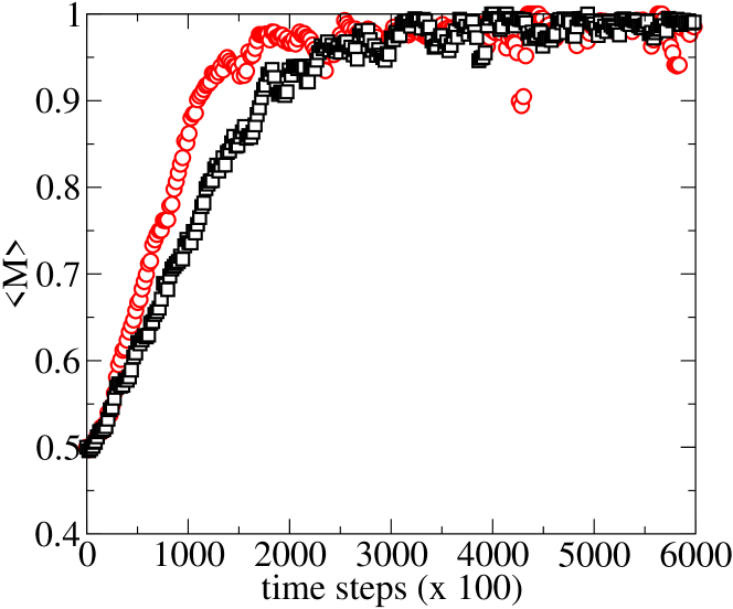
Figure 1: Average mobility $\langle M\rangle$ of predator (squares) and prey (circles) populations, as a function of time, for the first set of parameters. At the beginning ($t=0$) all individuals in both populations have the same mobility ($M=0.5$).

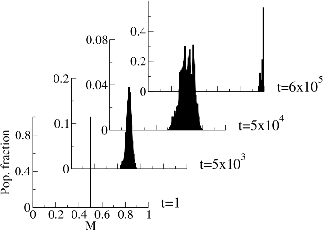
Figure 2: Mobility distributions of prey population (predator’s has similar behavior) for selected time steps, starting with concentrated distributions at time $t=0$. The set of parameters is the same as in figure 1.

The fact that we chose initial distributions for mobility concentrated around a single mobility value and that this distribution moved steadily to high $\langle M\rangle$ values suggests that the adaptive landscape is a simple one, with a single maximum near $\langle M\rangle=1$. It is worth inquiring further into the structure of the adaptive landscape by choosing a different initial condition: individuals are assigned random mobility values taken from an uniform distribution over the interval $[0,1]$. In this way, every region of the adaptive landscape is accessible to at least a few individuals; if a region contains an adaptation maximum it is very probable that the individuals in that region will form a significant fraction of the final population. On the other hand, individuals that happen to be around a minimum will most certainly disappear from the population relatively quickly. As Fig. 3 shows, the distribution is rapidly narrowed, once again evidencing a strong selective pressure in favor of high mobilities. Although we expected, from the previous results, the adaptive landscape to be simple, exhibiting a single maximum very near $\langle M\rangle=1$, we now see a hint of a more complex structure, with two maxima. Nevertheless both maxima correspond to very similar values of mobility, and may be artifacts of statistical fluctuations in finite populations.

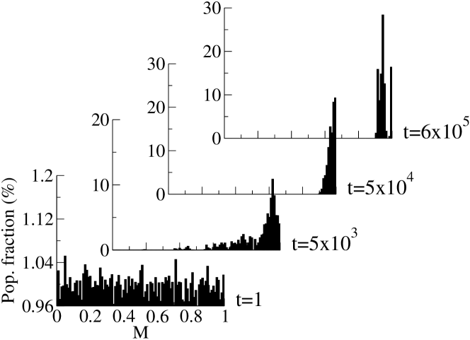
Figure 3: Mobility distributions of prey population (predator’s has similar behavior) for selected time steps, starting with uniform distributions at time $t=0$. The set of parameters is the same as in figure 1.

If we change the set of parameters regulating local dynamics, call it the second set, different evolutionary regimes may be observed, as shown in Fig. 4. There are outstanding differences between these results and those presented on Fig. 1: the saturation value reached by the average mobility is much smaller in this second case, as is its rate of change. This suggests that the selective pressure is less intense in this case. However, the smaller saturation value may have a diverse meaning: since we started with a concentrated mobility distribution and the mutation rate is relatively small, if the adaptive landscape has more than one maximum the population may be “trapped” in a local maximum, much like a dynamical system may become “trapped” in a metastable state. To settle the question we again resort to an initial distribution of mobilities that is uniform. Here we see that this situation is a bit more complex: the adaptive landscape displays multiple maxima indeed, as shown in Fig. 5. The lower saturation value we observed in Fig. 4 thus is a result of the population being trapped by the first maximum it encounters. Since the mutation rate $\sigma$ is relatively small, there is not enough variability for the population to overcome the adaptive valley before reaching for the next peak. We also have results showing that, if the mutation rate is increased slightly, the excess variability thus generated is enough for the transposition of the adaptive valley

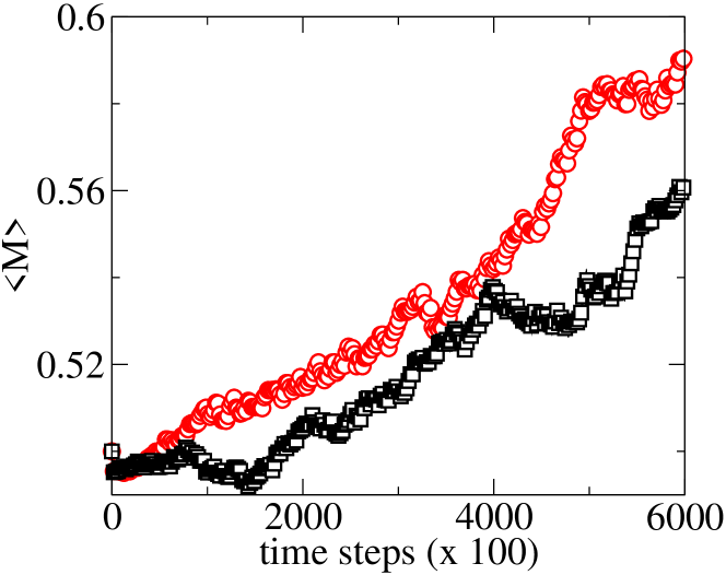
Figure 4: Average mobility $\langle M\rangle$ of predator (squares) and prey (circles) populations, as a function of time, for the second set of parameters. At the beginning ($t=0$) all individuals in both populations have the same mobility ($M=0.5$).

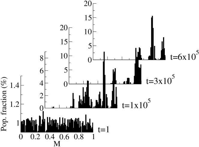
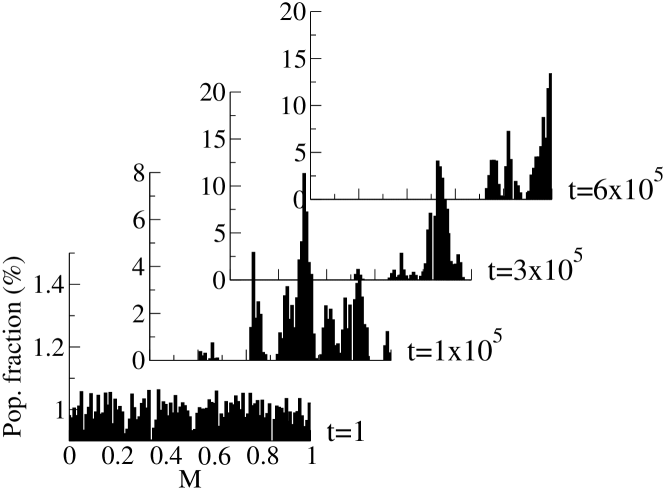
Figure 5: Mobility distributions of predator (top panel) and prey (bottom panel) populations for selected time steps, starting with uniform distributions at time $t=0$. The second set of parameters has been used. Notice that the asymptotic distributions display at least three distinct maxima, indicating a polymorphic population.

It is worth noticing that, besides its interesting evolutionary behavior, this model also exhibits pattern formation, that is, even though the dynamical rules are the same for the entire lattice, the resulting dynamics generates inhomogeneous population distributions. This is not, however, a consequence of the evolutionary mechanism but of the reaction-diffusion structure of the population dynamics. Nevertheless, the evolutionary mechanism affects significantly the features of the asymptotic patterns, and vice-versa. That this is so may be noticed from evidences of correlation between pattern formation and selective pressure. These can be seen in Fig. 6 where one sees that the selective pressure is stronger when the populations are distributed inhomogeneously in the environment. Reasoning naïvely one could argue that this result is somehow expected, since there is no apparent advantage in being more or less mobile in a homogeneous environment. However, as stated above, pattern formation is a consequence of dynamics, as much as the selective pressure in our model and, in some situations, introduction of the evolutionary mechanism changes qualitatively the population distribution, as can be seen in Fig. 7. Thus, the relation between pattern formation and selective pressure is by no means trivial, and deserves further investigation.

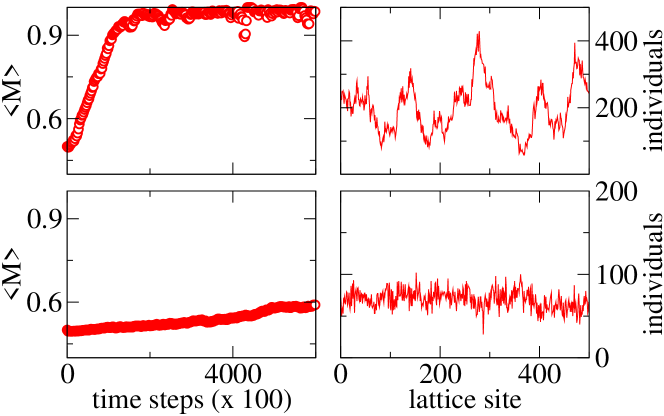
Figure 6: Time evolution of $\langle M\rangle$ (left panel) for preys and corresponding asymptotic spatial distribution (right panel) of prey populations, showing evidence of a correlation between heterogeneity in spatial distribution and strength of natural selection.

To summarize, we presented a model for two spatially distributed, co-evolving populations interacting via predator-prey local dynamics, in which natural selection appears spontaneously as a result of the system’s dynamics. We also showed that in some cases a complex adaptive landscape is generated dynamically, which may lead to the appearance of polymorphic populations. This state is the departure point for an important evolutionary process known as sympatric speciation. Incidentally we showed that this model displays pattern formation, which may be relevant to explain spontaneously fragmented habitats. We also showed evidence of a correlation between pattern formation and selective pressure, that needs to be better understood.

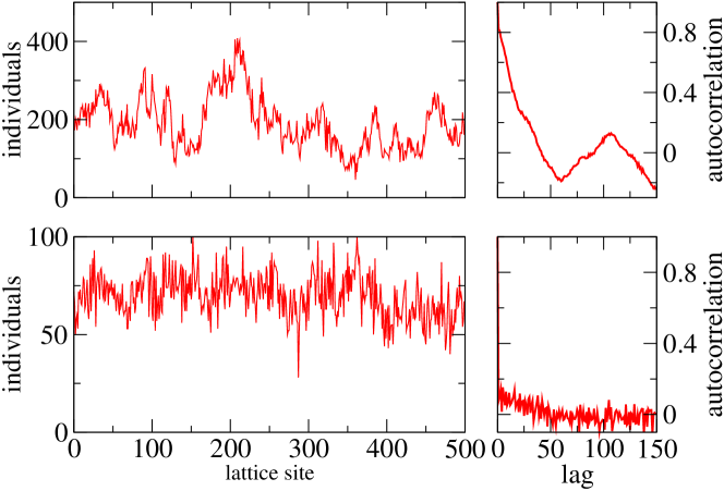
Figure 7: Asymptotic spatial distribution (left panel) of prey in the absence (top) and in the presence (bottom) of evolutionary mechanism. In the left panel, the spatial autocorrelation function in both cases show that the evolutionary mechanism changed qualitatively the spatial pattern, destroying the long-range order observed in the absence of evolution.

The authors acknowledge enlightening discussions with Thadeu J. P. Penna, Karen Luz-Burgoa, José Nogales, J. N. C. Louzada and Iraziet C. Charret. A.T.C. gratefully acknowledges Luciana J. Costa for many fruitful discussions and a critical reading of the manuscript. A.T.C. and M.P.D. acknowledge partial financial support from CNPq (Brazil). M.F.B.M. acknowledges partial financial support from CAPES (Brazil). The computational facilities in which part of this work was done were provided by FINEP (Brazil).

References

- (1) M. Turelli, N.H. Barton, and J.A. Coyne, Trends Ecol. Evol. 16, 330 (2001).
- (2) S. Via, Trends Ecol. Evol. 16, 381 (2001).
- (3) M.L. Friesen, G. Saxer, M. Travisano, and Michael Doebeli, Evolution 58, 245 (2004).
- (4) K. Luz-Burgoa, S.M. de Oliveira, J.S.S. Martins JSS, D. Stauffer and A.O. Sousa, Braz. J. Phys. 33, 623 (2003).
- (5) E. Mayr, Evolution and the Diversity of Life, The Belknap Press of Harvard University Press, London, 1997.
- (6) M. Ridley, Evolution, Second Edition, Blackwell Science, Oxford, 1996.
- (7) J.D. Murray, Mathematical Biology, 2nd Edition, Springer-Verlag, Berlin, 1998.
- (8) S.G.F. Martins, A.T. Costa Jr, J.S.S. Bueno Filho, and T.J.P. Penna, Int. J. Mod. Phys. C 12, 807 (2001).
- (9) C.P. Doncaster, G.E. Pound and S.J. Cox, Journal of Animal Ecology 72, 116 (2003).