Measuring Shared Information and Coordinated Activity in Neuronal Networks

Abstract

Most nervous systems encode information about stimuli in the responding activity of large neuronal networks. This activity often manifests itself as dynamically coordinated sequences of action potentials. Since multiple electrode recordings are now a standard tool in neuroscience research, it is important to have a measure of such network-wide behavioral coordination and information sharing, applicable to multiple neural spike train data. We propose a new statistic, informational coherence, which measures how much better one unit can be predicted by knowing the dynamical state of another. We argue informational coherence is a measure of association and shared information which is superior to traditional pairwise measures of synchronization and correlation. To find the dynamical states, we use a recently-introduced algorithm which reconstructs effective state spaces from stochastic time series. We then extend the pairwise measure to a multivariate analysis of the network by estimating the network multi-information. We illustrate our method by testing it on a detailed model of the transition from gamma to beta rhythms.

Much of the most important information in neural systems is shared over multiple neurons or cortical areas, in such forms as population codes and distributed representations [1]. On behavioral time scales, neural information is stored in temporal patterns of activity as opposed to static markers; therefore, as information is shared between neurons or brain regions, it is physically instantiated as coordination between entire sequences of neural spikes. Furthermore, neural systems and regions of the brain often require coordinated neural activity to perform important functions; acting in concert requires multiple neurons or cortical areas to share information [2]. Thus, if we want to measure the dynamic network-wide behavior of neurons and test hypotheses about them, we need reliable, practical methods to detect and quantify behavioral coordination and the associated information sharing across multiple neural units. These would be especially useful in testing ideas about how particular forms of coordination relate to distributed coding (e.g., that of [3]). Current techniques to analyze relations among spike trains handle only pairs of neurons, so we further need a method which is extendible to analyze the coordination in the network, system, or region as a whole. Here we propose a new measure of behavioral coordination and information sharing, informational coherence, based on the notion of dynamical state.

Section 1 argues that coordinated behavior in neural systems is often not captured by existing measures of synchronization or correlation, and that something sensitive to nonlinear, stochastic, predictive relationships is needed. Section 2 defines informational coherence as the (normalized) mutual information between the dynamical states of two systems and explains how looking at the states, rather than just observables, fulfills the needs laid out in Section 1. Since we rarely know the right states a prori, Section 2.1 briefly describes how we reconstruct effective state spaces from data. Section 2.2 gives some details about how we calculate the informational coherence and approximate the global information stored in the network. Section 3 applies our method to a model system (a biophysically detailed conductance-based model) comparing our results to those of more familiar second-order statistics. In the interest of space, we omit proofs and a full discussion of the existing literature, giving only minimal references here; proofs and references will appear in a longer paper now in preparation.

1 Synchrony or Coherence?

Most hypotheses which involve the idea that information sharing is reflected in coordinated activity across neural units invoke a very specific notion of coordinated activity, namely strict synchrony: the units should be doing exactly the same thing (e.g., spiking) at exactly the same time. Investigators then measure coordination by measuring how close the units come to being strictly synchronized (e.g., variance in spike times).

From an informational point of view, there is no reason to favor strict synchrony over other kinds of coordination. One neuron consistently spiking 50 ms after another is just as informative a relationship as two simultaneously spiking, but such stable phase relations are missed by strict-synchrony approaches. Indeed, whatever the exact nature of the neural code, it uses temporally extended patterns of activity, and so information sharing should be reflected in coordination of those patterns, rather than just the instantaneous activity.

There are three common ways of going beyond strict synchrony: cross-correlation and related second-order statistics, mutual information, and topological generalized synchrony.

The cross-correlation function (the normalized covariance function; this includes, for present purposes, the joint peristimulus time histogram [2]), is one of the most widespread measures of synchronization. It can be efficiently calculated from observable series; it handles statistical as well as deterministic relationships between processes; by incorporating variable lags, it reduces the problem of phase locking. Fourier transformation of the covariance function $\gamma_{XY}(h)$ yields the cross-spectrum $F_{XY}(\nu)$, which in turn gives the spectral coherence $c_{XY}(\nu)=F^{2}_{XY}(\nu)/F_{X}(\nu)F_{Y}(\nu)$, a normalized correlation between the Fourier components of $X$ and $Y$. Integrated over frequencies, the spectral coherence measures, essentially, the degree of linear cross-predictability of the two series. ([4] applies spectral coherence to coordinated neural activity.) However, such second-order statistics only handle linear relationships. Since neural processes are known to be strongly nonlinear, there is little reason to think these statistics adequately measure coordination and synchrony in neural systems.

Mutual information is attractive because it handles both nonlinear and stochastic relationships and has a very natural and appealing interpretation. Unfortunately, it often seems to fail in practice, being disappointingly small even between signals which are known to be tightly coupled [5]. The major reason is that the neural codes use distinct patterns of activity over time, rather than many different instantaneous actions, and the usual approach misses these extended patterns. Consider two neurons, one of which drives the other to spike 50 ms after it does, the driving neuron spiking once every 500 ms. These are very tightly coordinated, but whether the first neuron spiked at time $t$ conveys little information about what the second neuron is doing at $t$ — it’s not spiking, but it’s not spiking most of the time anyway. Mutual information calculated from the direct observations conflates the “no spike” of the second neuron preparing to fire with its just-sitting-around “no spike”. Here, mutual information could find the coordination if we used a 50 ms lag, but that won’t work in general. Take two rate-coding neurons with base-line firing rates of 1 Hz, and suppose that a stimulus excites one to 10 Hz and suppresses the other to 0.1 Hz. The spiking rates thus share a lot of information, but whether the one neuron spiked at $t$ is uninformative about what the other neuron did then, and lagging won’t help.

Generalized synchrony is based on the idea of establishing relationships between the states of the various units. “State” here is taken in the sense of physics, dynamics and control theory: the state at time $t$ is a variable which fixes the distribution of observables at all times $\geq t$, rendering the past of the system irrelevant [6]. Knowing the state allows us to predict, as well as possible, how the system will evolve, and how it will respond to external forces [7]. Two coupled systems are said to exhibit generalized synchrony if the state of one system is given by a mapping from the state of the other. Applications to data employ state-space reconstruction [8]: if the state $x\in\mathcal{X}$ evolves according to smooth, $d$-dimensional deterministic dynamics, and we observe a generic function $y=f(x)$, then the space $\mathcal{Y}$ of time-delay vectors $\left[y(t),y(t-\tau),...y(t-(k-1)\tau)\right]$ is diffeomorphic to $\mathcal{X}$ if $k>2d$, for generic choices of lag $\tau$. The various versions of generalized synchrony differ on how, precisely, to quantify the mappings between reconstructed state spaces, but they all appear to be empirically equivalent to one another and to notions of phase synchronization based on Hilbert transforms [5]. Thus all of these measures accommodate nonlinear relationships, and are potentially very flexible. Unfortunately, there is essentially no reason to believe that neural systems have deterministic dynamics at experimentally-accessible levels of detail, much less that there are deterministic relationships among such states for different units.

What we want, then, but none of these alternatives provides, is a quantity which measures predictive relationships among states, but allows those relationships to be nonlinear and stochastic. The next section introduces just such a measure, which we call “informational coherence”.

2 States and Informational Coherence

There are alternatives to calculating the “surface” mutual information between the sequences of observations themselves (which, as described, fails to capture coordination). If we know that the units are phase oscillators, or rate coders, we can estimate their instantaneous phase or rate and, by calculating the mutual information between those variables, see how coordinated the units’ patterns of activity are. However, phases and rates do not exhaust the repertoire of neural patterns and a more general, common scheme is desirable. The most general notion of “pattern of activity” is simply that of the dynamical state of the system, in the sense mentioned above. We now formalize this.

Assuming the usual notation for Shannon information [9], the information content of a state variable $X$ is $H[X]$ and the mutual information between $X$ and $Y$ is $I[X;Y]$. As is well-known, $I[X;Y]\leq\min{H[X],H[Y]}$. We use this to normalize the mutual state information to a $0-1$ scale, and this is the informational coherence (IC).

$$\psi(X,Y) = \frac{I[X;Y]}{\min{H[X],H[Y]}}~{},~{}~{}\mathrm{with}\ 0/0=0~{}.$$ (1)

$\psi$ can be interpreted as follows. $I[X;Y]$ is the Kullback-Leibler divergence between the joint distribution of $X$ and $Y$, and the product of their marginal distributions [9], indicating the error involved in ignoring the dependence between $X$ and $Y$. The mutual information between predictive, dynamical states thus gauges the error involved in assuming the two systems are independent, i.e., how much predictions could improve by taking into account the dependence. Hence it measures the amount of dynamically-relevant information shared between the two systems. $\psi$ simply normalizes this value, and indicates the degree to which two systems have coordinated patterns of behavior (cf. [10], although this only uses directly observable quantities).

2.1 Reconstruction and Estimation of Effective State Spaces

As mentioned, the state space of a deterministic dynamical system can be reconstructed from a sequence of observations. This is the main tool of experimental nonlinear dynamics [8]; but the assumption of determinism is crucial and false, for almost any interesting neural system. While classical state-space reconstruction won’t work on stochastic processes, such processes do have state-space representations [11], and, in the special case of discrete-valued, discrete-time series, there are ways to reconstruct the state space.

Here we use the CSSR algorithm, introduced in [12] (code available at http://bactra.org/CSSR). This produces causal state models, which are stochastic automata capable of statistically-optimal nonlinear prediction; the state of the machine is a minimal sufficient statistic for the future of the observable process[13]. The basic idea is to form a set of states which should be (1) Markovian, (2) sufficient statistics for the next observable, and (3) have deterministic transitions (in the automata-theory sense). The algorithm begins with a minimal, one-state, IID model, and checks whether these properties hold, by means of hypothesis tests. If they fail, the model is modified, generally but not always by adding more states, and the new model is checked again. Each state of the model corresponds to a distinct distribution over future events, i.e., to a statistical pattern of behavior. Under mild conditions, which do not involve prior knowledge of the state space, CSSR converges in probability to the unique causal state model of the data-generating process [12]. In practice, CSSR is quite fast (linear in the data size), and generalizes at least as well as training hidden Markov models with the EM algorithm and using cross-validation for selection, the standard heuristic [12].

One advantage of the causal state approach (which it shares with classical state-space reconstruction) is that state estimation is greatly simplified. In the general case of nonlinear state estimation, it is necessary to know not just the form of the stochastic dynamics in the state space and the observation function, but also their precise parametric values and the distribution of observation and driving noises. Estimating the state from the observable time series then becomes a computationally-intensive application of Bayes’s Rule [17].

Due to the way causal states are built as statistics of the data, with probability 1 there is a finite time, $t$, at which the causal state at time $t$ is certain. This is not just with some degree of belief or confidence: because of the way the states are constructed, it is impossible for the process to be in any other state at that time. Once the causal state has been established, it can be updated recursively, i.e., the causal state at time $t+1$ is an explicit function of the causal state at time $t$ and the observation at $t+1$. The causal state model can be automatically converted, therefore, into a finite-state transducer which reads in an observation time series and outputs the corresponding series of states [18, 13]. (Our implementation of CSSR filters its training data automatically.) The result is a new time series of states, from which all non-predictive components have been filtered out.

2.2 Estimating the Coherence

Our algorithm for estimating the matrix of informational coherences is as follows. For each unit, we reconstruct the causal state model, and filter the observable time series to produce a series of causal states. Then, for each pair of neurons, we construct a joint histogram of the state distribution, estimate the mutual information between the states, and normalize by the single-unit state informations. This gives a symmetric matrix of $\psi$ values.

Even if two systems are independent, their estimated IC will, on average, be positive, because, while they should have zero mutual information, the empirical estimate of mutual information is non-negative. Thus, the significance of IC values must be assessed against the null hypothesis of system independence. The easiest way to do so is to take the reconstructed state models for the two systems and run them forward, independently of one another, to generate a large number of simulated state sequences; from these calculate values of the IC. This procedure will approximate the sampling distribution of the IC under a null model which preserves the dynamics of each system, but not their interaction. We can then find $p$-values as usual. We omit them here to save space.

2.3 Approximating the Network Multi-Information

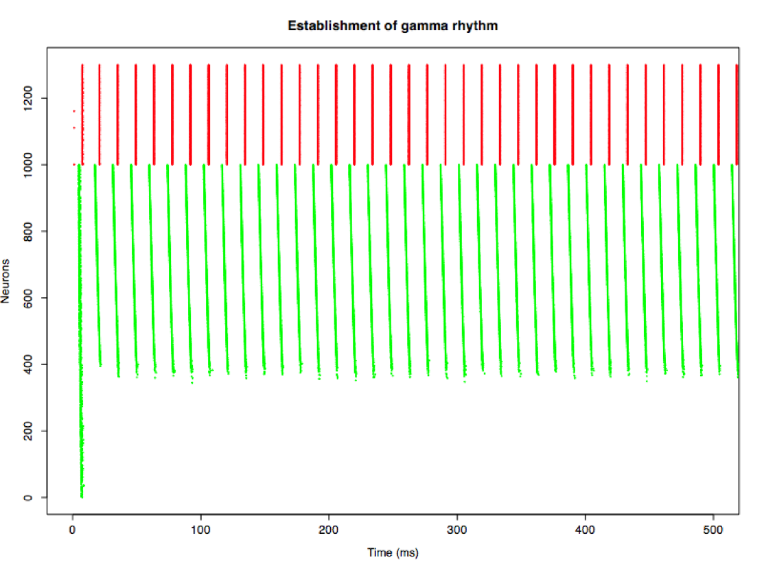
$a$ $b$

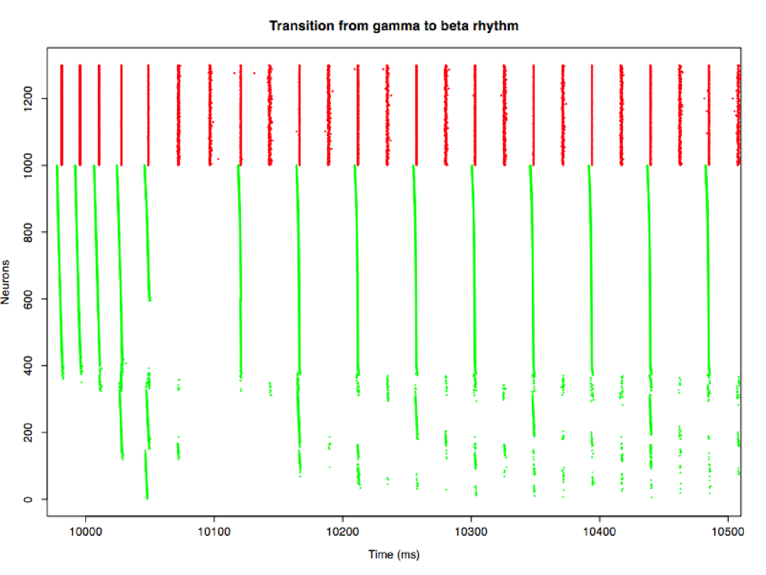
Figure 1: Rastergrams of neuronal spike-times in the network. Excitatory, pyramidal neurons (numbers 1 to 1000) are shown in green, inhibitory interneurons (numbers 1001 to 1300) in red. During the first 10 seconds ($a$), the current connections among the pyramidal cells are suppressed and a gamma rhythm emerges (left). At $t=10\mathrm{s}$, those connections become active, leading to a beta rhythm ($b$, right).

There is broad agreement [2] that analyses of networks should not just be an analysis of pairs of neurons, averaged over pairs. Ideally, an analysis of information sharing in a network would look at the over-all structure of statistical dependence between the various units, reflected in the complete joint probability distribution $P$ of the states. This would then allow us, for instance, to calculate the $n$-fold multi-information, $I[X_{1},X_{2},\ldots X_{n}]\equiv D(P||Q)$, the Kullback-Leibler divergence between the joint distribution $P$ and the product of marginal distributions $Q$, analogous to the pairwise mutual information [19]. Calculated over the predictive states, the multi-information would give the total amount of shared dynamical information in the system. Just as we normalized the mutual information $I[X_{1},X_{2}]$ by its maximum possible value, $\min{H[X_{1}],H[X_{2}]}$, we normalize the multi-information by its maximum, which is the smallest sum of $n-1$ marginal entropies:

$$I[X_{1};X_{2};\ldots X_{n}]\leq\min_{k}{\sum_{i\neq k}{H[X_{n}]}}$$

Unfortunately, $P$ is a distribution over a very high dimensional space and so, hard to estimate well without strong parametric constraints. We thus consider approximations.

The lowest-order approximation treats all the units as independent; this is the distribution $Q$. One step up are tree distributions, where the global distribution is a function of the joint distributions of pairs of units. Not every pair of units needs to enter into such a distribution, though every unit must be part of some pair. Graphically, a tree distribution corresponds to a spanning tree, with edges linking units whose interactions enter into the global probability, and conversely spanning trees determine tree distributions. Writing $E_{T}$ for the set of pairs $(i,j)$ and abbreviating $X_{1}=x_{1},X_{2}=x_{2},\ldots X_{n}=x_{n}$ by $\mathbf{X}=\mathbf{x}$, one has

$$T(\mathbf{X}=\mathbf{x})=\prod_{(i,j)\in E_{T}}{\frac{T(X_{i}=x_{i},X_{j}=x_{j})}{T(X_{i}=x_{i})T(X_{j}=x_{j})}}\prod_{i=1}^{n}{T(X_{i}=x_{i})}$$ (2)

where the marginal distributions $T(X_{i})$ and the pair distributions $T(X_{i},X_{j})$ are estimated by the empirical marginal and pair distributions.

We must now pick edges $E_{T}$ so that $T$ best approximates the true global distribution $P$. A natural approach is to minimize $D(P||T)$, the divergence between $P$ and its tree approximation. Chow and Liu [20] showed that the maximum-weight spanning tree gives the divergence-minimizing distribution, taking an edge’s weight to be the mutual information between the variables it links.

There are three advantages to using the Chow-Liu approximation. (1) Estimating $T$ from empirical probabilities gives a consistent maximum likelihood estimator of the ideal Chow-Liu tree [20], with reasonable rates of convergence, so $T$ can be reliably known even if $P$ cannot. (2) There are efficient algorithms for constructing maximum-weight spanning trees, such as Prim’s algorithm [21, sec. 23.2], which runs in time $O(n^{2}+n\log{n})$. Thus, the approximation is computationally tractable. (3) The KL divergence of the Chow-Liu distribution from $Q$ gives a lower bound on the network multi-information; that bound is just the sum of the mutual informations along the edges in the tree:

$$I[X_{1};X_{2};\ldots X_{n}]\geq D(T||Q)=\sum_{(i,j)\in E_{T}}{I[X_{i};X_{j}]}$$ (3)

Even if we knew $P$ exactly, Eq. 3 would be useful as an alternative to calculating $D(P||Q)$ directly, evaluating $\log{P(\mathbf{x})/Q(\mathbf{x})}$ for all the exponentially-many configurations $\mathbf{x}$.

It is natural to seek higher-order approximations to $P$, e.g., using three-way interactions not decomposable into pairwise interactions [22, 19]. But it is hard to do so effectively, because finding the optimal approximation to $P$ when such interactions are allowed is NP [23], and analytical formulas like Eq. 3 generally do not exist [19]. We therefore confine ourselves to the Chow-Liu approximation here.

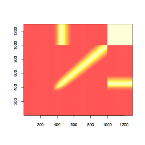
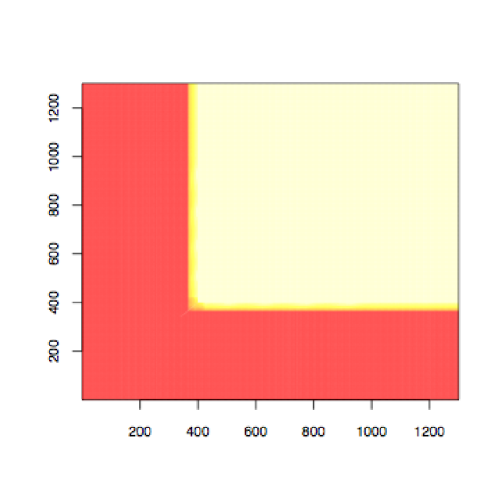
a b
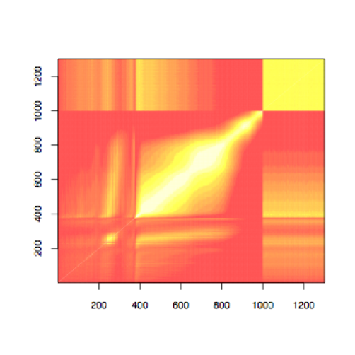
c d

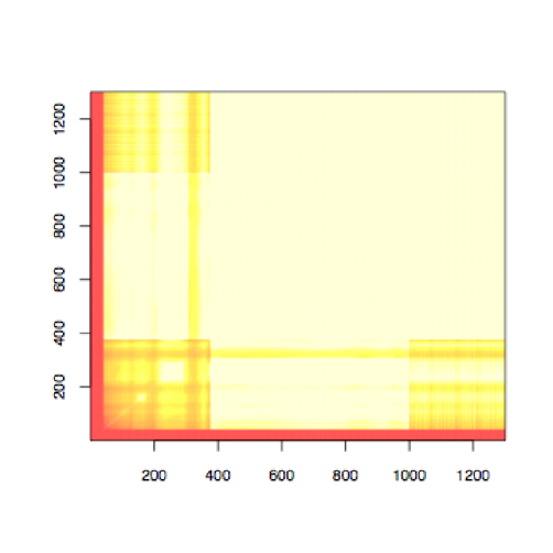
Figure 2: Heat-maps of coordination for the network, as measured by zero-lag cross-correlation (top row) and informational coherence (bottom), contrasting the gamma rhythm (left column) with the beta (right). Colors run from red (no coordination) through yellow to pale cream (maximum).

3 Example: A Model of Gamma and Beta Rhythms

We use simulated data as a test case, instead of empirical multiple electrode recordings, which allows us to try the method on a system of over 1000 neurons and compare the measure against expected results. The model, taken from [24], was originally designed to study episodes of gamma (30–80Hz) and beta (12–30Hz) oscillations in the mammalian nervous system, which often occur successively with a spontaneous transition between them. More concretely, the rhythms studied were those displayed by in vitro hippocampal (CA1) slice preparations and by in vivo neocortical EEGs.

The model contains two neuron populations: excitatory (AMPA) pyramidal neurons and inhibitory (GABA${}_{\mbox{{A}}}$) interneurons, defined by conductance-based Hodgkin-Huxley-style equations. Simulations were carried out in a network of 1000 pyramidal cells and 300 interneurons. Each cell was modeled as a one-compartment neuron with all-to-all coupling, endowed with the basic sodium and potassium spiking currents, an external applied current, and some Gaussian input noise.

The first 10 seconds of the simulation correspond to the gamma rhythm, in which only a group of neurons is made to spike via a linearly increasing applied current. The beta rhythm (subsequent 10 seconds) is obtained by activating pyramidal-pyramidal recurrent connections (potentiated by Hebbian preprocessing as a result of synchrony during the gamma rhythm) and a slow outward after-hyper-polarization (AHP) current (the M-current), suppressed during gamma due to the metabotropic activation used in the generation of the rhythm. During the beta rhythm, pyramidal cells, silent during gamma rhythm, fire on a subset of interneurons cycles (Fig. 1).

Fig. 2 compares zero-lag cross-correlation, a second-order method of quantifying coordination, with the informational coherence calculated from the reconstructed states. (In this simulation, we could have calculated the actual states of the model neurons directly, rather than reconstructing them, but for purposes of testing our method we did not.) Cross-correlation finds some of the relationships visible in Fig. 1, but is confused by, for instance, the phase shifts between pyramidal cells. (Surface mutual information, not shown, gives similar results.) Informational coherence, however, has no trouble recognizing the two populations as effectively coordinated blocks. The presence of dynamical noise, problematic for ordinary state reconstruction, is not an issue. The average IC is $0.411$ (or $0.797$ if the inactive, low-numbered neurons are excluded). The tree estimate of the global informational multi-information is $3243.7$ bits, with a global coherence of $0.777$. The right half of Fig. 2 repeats this analysis for the beta rhythm; in this stage, the average IC is $0.614$, and the tree estimate of the global multi-information is $7377.7$ bits, though the estimated global coherence falls very slightly to $0.742$. This is because low-numbered neurons which were quiescent before are now active, contributing to the global information, but the over-all pattern is somewhat weaker and more noisy (as can be seen from Fig. 1$b$.) So, as expected, the total information content is higher, but the overall coordination across the network is lower.

4 Conclusion

Informational coherence provides a measure of neural information sharing and coordinated activity which accommodates nonlinear, stochastic relationships between extended patterns of spiking. It is robust to dynamical noise and leads to a genuinely multivariate measure of global coordination across networks or regions. Applied to data from multi-electrode recordings, it should be a valuable tool in evaluating hypotheses about distributed neural representation and function.

Acknowledgments

Thanks to R. Haslinger, E. Ionides and S. Page; and for support to the Santa Fe Institute (under grants from Intel, the NSF and the MacArthur Foundation, and DARPA agreement F30602-00-2-0583), the Clare Booth Luce Foundation (KLK) and the James S. McDonnell Foundation (CRS).

References

- [1] L. F. Abbott and T. J. Sejnowski, eds. Neural Codes and Distributed Representations. MIT Press, 1998.
- [2] E. N. Brown, R. E. Kass, and P. P. Mitra. Nature Neuroscience, 7:456–461, 2004.
- [3] D. H. Ballard, Z. Zhang, and R. P. N. Rao. In R. P. N. Rao, B. A. Olshausen, and M. S. Lewicki, eds., Probabilistic Models of the Brain, pp. 273–284, MIT Press, 2002.
- [4] D. R. Brillinger and A. E. P. Villa. In D. R. Brillinger, L. T. Fernholz, and S. Morgenthaler, eds., The Practice of Data Analysis, pp. 77–92. Princeton U.P., 1997.
- [5] R. Quian Quiroga et al. Physical Review E, 65:041903, 2002.
- [6] R. F. Streater. Statistical Dynamics. Imperial College Press, London.
- [7] M. L. Littman, R. S. Sutton, and S. Singh. In T. G. Dietterich, S. Becker, and Z. Ghahramani, eds., Advances in Neural Information Processing Systems 14, pp. 1555–1561. MIT Press, 2002.
- [8] H. Kantz and T. Schreiber. Nonlinear Time Series Analysis. Cambridge U.P., 1997.
- [9] T. M. Cover and J. A. Thomas. Elements of Information Theory. Wiley, 1991.
- [10] M. Palus et al. Physical Review E, 63:046211, 2001.
- [11] F. B. Knight. Annals of Probability, 3:573–596, 1975.
- [12] C. R. Shalizi and K. L. Shalizi. In M. Chickering and J. Halpern, eds., Uncertainty in Artificial Intelligence: Proceedings of the Twentieth Conference, pp. 504–511. AUAI Press, 2004.
- [13] C. R. Shalizi and J. P. Crutchfield. Journal of Statistical Physics, 104:817–819, 2001.
- [14] H. Jaeger. Neural Computation, 12:1371–1398, 2000.
- [15] D. Ron, Y. Singer, and N. Tishby. Machine Learning, 25:117–149, 1996.
- [16] P. Bühlmann and A. J. Wyner. Annals of Statistics, 27:480–513, 1999.
- [17] N. U. Ahmed. Linear and Nonlinear Filtering for Scientists and Engineers. World Scientific, 1998.
- [18] D. R. Upper. PhD thesis, University of California, Berkeley, 1997.
- [19] E. Schneidman, S. Still, M. J. Berry, and W. Bialek. Physical Review Letters, 91:238701, 2003.
- [20] C. K. Chow and C. N. Liu. IEEE Transactions on Information Theory, IT-14:462–467, 1968.
- [21] T. H. Cormen et al. Introduction to Algorithms. 2nd ed. MIT Press, 2001.
- [22] S. Amari. IEEE Transacttions on Information Theory, 47:1701–1711, 2001.
- [23] S. Kirshner, P. Smyth, and A. Robertson. Tech. Rep. 04-04, UC Irvine, Information and Computer Science, 2004.
- [24] M. S. Olufsen et al. Journal of Computational Neuroscience, 14:33–54, 2003.