Asymptotic construction of pulses in the discrete Hodgkin-Huxley model for myelinated nerves

Abstract

A quantitative description of pulses and wave trains in the spatially discrete Hodgkin-Huxley model for myelinated nerves is given. Predictions of the shape and speed of the waves and the thresholds for propagation failure are obtained. Our asymptotic predictions agree quite well with numerical solutions of the model and describe wave patterns generated by repeated firing at a boundary.

I Introduction

Understanding wave propagation in discrete excitable media is challenging because of poorly understood phenomena associated with spatial discreteness sleeman ; cbfhn ; keener1 ; fath ; cbn . The study of the transmission of nerve impulses along myelinated axons is a paradigmatic example. Myelinated nerve fibers, such as the motor axons of vertebrates, are covered almost everywhere by a thick insulating coat of myelin. Only a fraction of the active membrane is exposed, at small active nodes called Ranvier nodes. The myelinated axons of motor nerves can be very long, and contain hundreds or thousands of nodes biophys . The wave activity jumps from one node to the next one giving rise to “saltatory” propagation of impulses rushton . Saltatory conduction on myelinated nerve models has two important features. One is the possibility of increasing the speed of the nerve impulse while decreasing the diameter of the nerve fiber scott1 . The other is propagation failure when the myelin coat is damaged nature , which causes diseases such as multiple sclerosis.

The propagation of nerve impulses along a myelinated fiber can be described by the spatially discrete Hodgkin-Huxley system (HH) scott1 ; keener2 . For typical experimental data, this system couples equations for two fast variables and two slow variables. Most analytical studies of action potentials have focused on discrete FitzHugh-Nagumo (FHN) models for one fast and one slow variables kunov ; erneux2 ; sleeman ; hastings ; cbfhn ; tonnelier and discrete bistable equations for the leading edge richer ; zinner ; keener1 ; erneux1 ; fath ; cbn . Careful computational studies of models including more biological detail were carried out in fh ; goldman ; moore78 .

Numerical simulations show that reduced models involving only one fast and one slow variables are quantitatively inaccurate. Fig. 1 compares pulse solutions of the full discrete Hodgkin-Huxley model (circles) and a FitzHugh-Nagumo type reduction (asterisks) generated by exciting the left end of a fiber. The pulse solutions of the HH model are slower and narrower than the pulse solutions of the FHN-like reduction. Discarding one of the two fast variables produces a pulse with an increased speed, as illustrated by Figure 1. To describe the propagation of the pulse leading edge we need to keep the two fast variables. Their evolution is described by a discrete bistable equation coupled to an ordinary differential equation. This system yields a Nagumo type equation (a single discrete bistable equation) only in a very particular limit. Similarly, discarding one of the slow variables produces a slightly wider pulse than the one described by the two original slow variables. Moreover, FHN pulses and HH pulses have different structures. Pulse solutions of FHN-like models typically consist of two rigidly moving wave fronts cbfhn . HH pulses are “triangular waves”: they are formed by a leading wave front followed by a smooth region, as shown in Figure 1.

In this paper we introduce an asymptotic strategy to construct solitary pulses and wave trains in the discrete HH model. Our asymptotic study exploits time scale separation to split the variables in two blocks. The leading edge of the pulses is a wave front solution of the reduced system involving the two fast variables. This selects the speed of the wave. The two slow variables become relevant to determine the width of the peaks. Our asymptotic constructions agree reasonably well with numerical solutions for typical experimental data. For continuous HH models, a quantitative approximation scheme exploiting time scale separation was proposed in muratov . In the discrete case, traveling impulses do not appear as solutions of ordinary differential equations. Instead, more complicated differential-difference equations have to be analyzed.

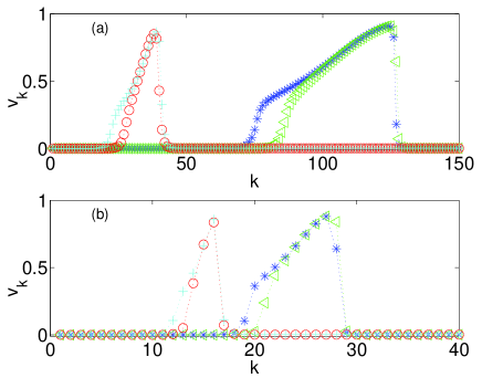
Figure 1: Comparison of pulses for the HH model (1)-(7) (circles), HH with $h_{k}+n_{k}=h^{*}+n^{*}$ (crosses), HH with $m_{k}=m_{\infty}(v_{k})$ (triangles) and the FHN-like system (8)-(9) (asterisks): (a) $D=0.09$, (b) $D=0.01$. The pulses have been generated by a short stimulation at $k=0$ and have been superimposed at a fixed time $t$. The pulse advances faster when only one fast variable is kept (asterisks and triangles). All variables are expressed in dimensionless units.

The paper is organized as follows. In Section II we describe the discrete Hodgkin-Huxley model for myelinated nerves. We present a few numerical solutions and discuss the reasons for the poor performance of FitzHugh-Nagumo type reductions. Solitary pulses are constructed in Section III. Section IV studies wave train generation at the boundary by periodic firing. In Section V, we describe the two main mechanisms for propagation failure, related to damage in the myelin sheath and the action of chemicals. Section VI contains our conclusions. In Appendix A we recall the derivation of the model. Appendix B explains the nondimensionalization procedure. Appendices C, D and E contain additional material on pulses.

II The Hodgkin-Huxley model for myelinated nerves

II.1 Dimensionless equations

The dimensionless Hodgkin-Huxley (HH) model for a myelinated nerve axon is:

$${dv_{k}\over dt}+I(v_{k},m_{k},n_{k},h_{k})=D(v_{k+1}-2v_{k}+v_{k-1}),$$ (1)

$${dm_{k}\over dt}=\Lambda_{m}(v_{k})\big{[}m_{\infty}(v_{k})-m_{k}\big{]},$$ (2)

$${dn_{k}\over dt}=\epsilon\Lambda_{n}(v_{k})\big{[}n_{\infty}(v_{k})-n_{k}\big{]},$$ (3)

$${dh_{k}\over dt}=\epsilon\lambda\Lambda_{h}(v_{k})\big{[}h_{\infty}(v_{k})-h_{k}\big{]},$$ (4)

with

$$\begin{array}[]{lcl}I(v,m,n,h)&=&g_{K}n^{4}(v-{V}_{K})+{g}_{Na}m^{3}h(v-1)\\ &&+{g}_{L}(v-{V}_{L}).\end{array}$$ (7)

Here, $v_{k}$ is the ratio of the deviation from rest of the membrane potential to a reference potential, $n_{k}$ is the potassium activation, $m_{k}$ is the sodium activation and $h_{k}$ the sodium inactivation. Appendix A recalls the derivation of the model. Appendix B details the procedure we have followed to nondimensionalize the system. The time scale is chosen by looking at the relaxation times $\tau_{n}$, $\tau_{m}$ and $\tau_{h}$ for $n_{k}$, $m_{k}$ and $h_{k}$. Typically, $\tau_{m}\ll\tau_{n}$ and $\tau_{n}\sim\tau_{h}$. Thus, $\epsilon={\tau_{m}\over\tau_{n}}$ is small.

The rate functions and the stationary states in (2)-(4) can be fitted to experimental data. Figure 2 plots their shape for the motor axon of a frog. Analytic expressions for these functions and typical values of the parameters for the frog nerve are collected in Appendix B and will be used in our numerical tests. The values for $g_{Na},g_{K},g_{L}$ have orders of magnitude $1,10^{-1},10^{-2}$, respectively. The coupling parameter $D\sim 10^{-1}$ and $\epsilon\sim 10^{-2}$ with $\lambda\sim 1$. This means that we have two separate time scales and that discreteness effects are relevant.

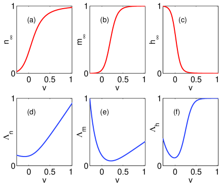
Figure 2: Coefficient functions in the HH equations as functions of $v_{k}=v$, in dimensionless units.

II.2 Numerical solutions

System (1)-(4) displays excitable behavior when it has a unique constant stationary state $(v^{*},m^{*},n^{*},h^{*})$, which is stable. Figures 3 and 4 show solitary pulses and wave train solutions generated by solving (1)-(4) numerically for the parameter values in Appendix B. After a short transient, the system relaxes to a traveling wave: $v_{k}(t)=v(k-ct)$, $m_{k}(t)=m(k-ct)$, $n_{k}(t)=n(k-ct)$ and $h_{k}(t)=h(k-ct)$. All nodes undergo the same evolution with a time delay ${1\over c}$.

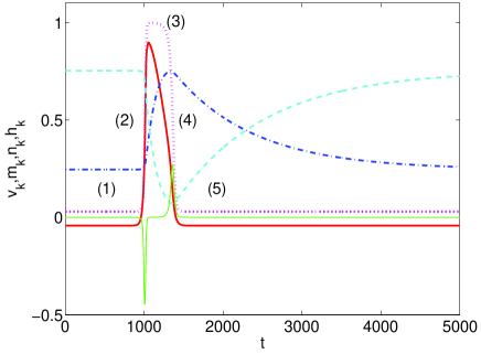
Figure 3: Temporal action potential $v_{k}(t)$ (thick solid line) generated by a single stimulation at $k=0$. The temporal profiles of $m_{k}$ (dotted), $n_{k}$ (dashed-dotted), $h_{k}$ (dashed) have been superimposed, all of them at a fixed node $k$. The thin solid line shows the profile of $m_{k}-m_{\infty}(v_{k})$. All variables are expressed in dimensionless units.

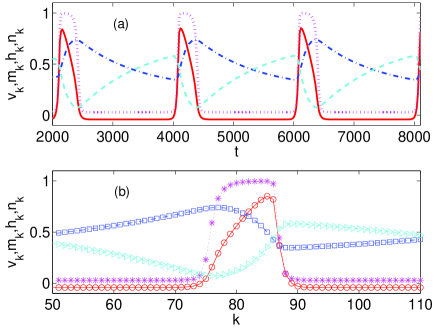
Figure 4: (a) Same as in Fig. 3 but generated by a periodic stimulation at $k=0$. (b) Corresponding spatial profiles at a fixed time: $v_{k}$ (circles), $m_{k}$ (asterisks), $n_{k}$ (squares), $h_{k}$ (triangles). Zoom in one spatial period. All variables are expressed in dimensionless units.

As shown in Figures 3 and 4, pulses and wave trains are composed of “sharp” interfaces and “smooth” regions. Let us describe the temporal profiles of a pulse as we move from left to right starting from the equilibrium region (1) in Figure 3. The leading edge of each pulse is a sharp interface, marked as (2) in Fig. 3. At this leading interface, $n_{k}$ and $h_{k}$ remain almost constant whereas $v_{k}$ and $m_{k}$ undergo abrupt changes. The evolution of $v_{k}$ and $m_{k}$ is described by a reduced bistable system and the leading edge is a wave front solution of this system. A smooth region follows, where $n_{k},h_{k}$ vary slowly and $v_{k}$ and $m_{k}$ are quasi-static: $m_{k}=m_{\infty}(v_{k})$ and $I(v_{k},m_{\infty}(v_{k});n_{k},m_{k})=0$. It is marked as (3) in Fig. 3. At the end of this region the approximation $m_{k}=m_{\infty}(v_{k})$ breaks down, see the thin solid line in Figure 3. A trailing interface develops, where $m_{k}$ changes abruptly whereas $n_{k},h_{k}$ remain almost constant. This new region is marked as (4) in Fig. 3. Notice that the fast variable $v_{k}$ happens to be near its equilibrium value $v^{*}$ and decreases smoothly towards it. Diffusion is negligible and the evolution of $v_{k}$ and $m_{k}$ at the trailing edge is governed by a system of ordinary differential equations. The bistable structure is lost and no trailing wave front is formed.

The variables seem to be split in two blocks: slow (evolving in the dimensionless time scale $T=\epsilon t$) and fast (evolving in the dimensionless time scale $t$). This suggest the possibility of finding an asymptotic description of pulses by exploiting time scale separation. The difficulty of dealing with a discrete space variable is overcome by noticing that the traveling wave profiles are smooth functions of a continuous variable and solve a set of differential-difference equations (see Appendix C). Let us first check whether the number of variables can be reduced.

II.3 Failure of simple FitzHugh-Nagumo type reductions

It is quite tempting to look for a simple asymptotic description of pulses in terms of one fast and one slow variable, as in the FitzHugh-Nagumo model fhn ; cbfhn . These reduced models usually assume that $m_{k}$ relaxes instantaneously to its equilibrium state $m_{k}=m_{\infty}(v_{k})$ and that the sum of the two slow variables is constant during an action potential $n_{k}+h_{k}=r$ keener2 :

$${dv_{k}\over dt}+g_{K}n_{k}^{4}(v_{k}\!-\!{V}_{K})\!+\!{g}_{Na}m_{\infty}(v_{k})^{3}(r-n_{k})(v_{k}\!-\!1)$$

$$\!+\!{g}_{L}(v_{k}\!-\!{V}_{L})=D(v_{k+1}-2v_{k}+v_{k-1}),$$ (8)

$${dn_{k}\over dt}=\epsilon\Lambda_{n}(v_{k})\big{[}n_{\infty}(v_{k})-n_{k}\big{]}.$$ (9)

In view of the numerical results described in Section II.2, these assumptions are inaccurate. The solid line in Fig. 3 shows that the difference $m_{k}-m_{\infty}(v_{k})$ is not negligible at the leading wave front. Setting $m_{k}=m_{\infty}(v_{k})$ distorts the speed, as shown in Figure 1. On the other hand, $n_{k}+h_{k}$ is not constant during at action potential. We may select $r=n^{*}+h^{*}$ to fit the leading edge but a slightly different value of $r$ is required for the trailing part of the pulse. Keeping $n_{k}+h_{k}=r$ during the action potential alters the width of the pulse, as shown in Figure 1.

In conclusion, the FHN type reduction (8)-(9) may be useful to gain insight on pulse motion and propagation failure in excitable media, but it is quantitatively inaccurate for the HH system with realistic parameter values.

III Asymptotic construction of pulses

Accurate descriptions of pulse waves in the HH model have to deal with the full set of equations. In this Section, we find an approximation of their temporal profiles by matched asymptotic expansions as $\epsilon\rightarrow 0$. This construction yields predictions for the speed and width of the pulses, as well as a characterization of the parameter ranges in which propagation fails. We explain the procedure for the parameter values indicated in (74). The structure of the pulse may change slightly for other parameter values. Other possible structures are discussed in Appendix E.

In a traveling pulse we distinguish five regions (illustrated in Figure 3). In each of them, a reduced description holds. The whole profile is reconstructed by matching the approximated solutions found in each region at zeroth order (see lager for a description of this technique). Our reference time scale is the slow time scale $T=\epsilon t$. The technical details of the matching are given in Appendix D.

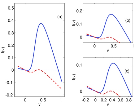
Figure 5: Shape of the source $f(v)$: (a) $g_{Na}=1.49$, (b) $g_{Na}=0.745$, (c) $g_{Na}=0.497$, when $(n,h)=(n^{*},h^{*})$ (solid line) and $(n,h)=(n^{[1]},h^{[1]})$ (dashed line). All variables are expressed in dimensionless units.

The resulting temporal pulse profiles with $k$ fixed have the following structure:

1. Front of the pulse. This is region (1) in Figure 3. Here $v_{k}\sim v^{*}$, $m_{k}\sim m^{*}$, $n_{k}\sim n^{*}$ and $h_{k}\sim h^{*}$, $(v^{*},m^{*},n^{*},h^{*})$ being the stable equilibrium state of the system.

2. Leading edge of the pulse, located at $T=T_{0}$ and marked as (2) in Figure 3. The slow variables, $n_{k}$ and $h_{k}$, remain essentially constant but the fast variables, $v_{k}$ and $m_{k}$, undergo rapid changes in the time scale $\overline{t}={T-T_{0}\over\epsilon}\in(-\infty,\infty)$. To leading order,

   $$\begin{array}[]{lll}{dv_{k}\over d\overline{t}}+I(v_{k},m_{k},n_{k},h_{k})=D(v_{k+1}-2v_{k}+v_{k-1}),\\ {dm_{k}\over d\overline{t}}=\Lambda_{m}(v_{k})\big{[}m_{\infty}(v_{k})-m_{k}\big{]},\\ {dn_{k}\over d\overline{t}}=0,\quad{dh_{k}\over d\overline{t}}=0,\end{array}$$ (13)

   Thus, $n_{k}$ and $n_{k}$ remain almost constant. Matching with the previous region, $n_{k}=n^{*}$ and $h_{k}=h^{*}$ (see Appendix D). The evolution of $v_{k}$ and $m_{k}$ is described by the ‘fast reduced system’:

   $${dv_{k}\over d\overline{t}}+I(v_{k},m_{k},n_{k},h_{k})=D(v_{k+1}-2v_{k}+v_{k-1}),$$ (14)

   $${dm_{k}\over d\overline{t}}=\Lambda_{m}(v_{k})\big{[}m_{\infty}(v_{k})-m_{k}\big{]},$$ (15)

   with $n_{k}=n^{*}$ and $h_{k}=h^{*}$. This system displays bistable behavior. Let us denote by $v=\nu^{(i)}(n,h),i=1,2,3$ the three solutions of

   $$f(v;n,h)=-I(v,m_{\infty}(v),n,h)=0$$ (16)

   in a neighborhood of $(n^{*},h^{*})$. The system (14)-(15) has a unique stable traveling wave front solution $v_{k}(t)=v(k-c\overline{t})$, $m_{k}=m(k-c\overline{t})$ joining the two stable constant states $\nu^{(3)}(n^{*},h^{*})$, $m_{\infty}(\nu^{(3)})$ and $\nu^{(1)}(n^{*},h^{*})$, $m_{\infty}(\nu^{(1)})$, which propagates with a definite speed $c=c_{+}(n^{*},h^{*})$. This wave front solution is the leading edge of the pulse.

3. Top of the pulse. This is region (3) in Figure 3. Here, the slow variables evolve in the time scale $T$ and the fast variables relax instantaneously to their equilibrium values: $m_{k}=m_{\infty}(v_{k})$, in which $v_{k}$ solves $f(v_{k};n_{k},h_{k})=0$. The evolution of the slow variables is governed by the ’slow reduced system’:

   $$\begin{array}[]{l}{dn_{k}\over dT}\!=\!\Lambda_{n}(v_{k})\big{[}n_{\infty}(v_{k})\!-\!n_{k}\big{]},\\ {dh_{k}\over dT}\!=\!\lambda\Lambda_{h}(v_{k})\big{[}h_{\infty}(v_{k})\!-\!h_{k}\big{]},\end{array}$$ (19)

   for $T_{0}<T<T_{1}$. Matching with the previous stage we get $v_{k}=\nu^{(3)}(n_{k},h_{k})$, $n_{k}=n^{*}$ and $h_{k}=h^{*}$ at $T=T_{0}$ (see Appendix D). For the parameter values indicated in (74), the third branch of roots $v_{k}=\nu^{(3)}(n_{k},h_{k})$ of $f(v_{k};n_{k},h_{k})=0$ disappears at $(n_{k},h_{k})=(n^{[1]},h^{[1]})$, colliding with the second branch: $\nu^{(3)}(n^{[1]},h^{[1]})=\nu^{(2)}(n^{[1]},h^{[1]})=v^{[1]}$. At the corresponding time $T=T_{1}$, region (3) ends. The time $T_{1}$ is characterized by $n_{k}(T_{1})=n^{[1]}$ and $h_{k}(T_{1})=h^{[1]}$ nota .

4. Trailing edge of the pulse, located at $T_{1}$ and marked as (4) in Figure 3. In this region, $v_{k}$ is no longer at equilibrium since the two largest roots of $f(v;n_{k},h_{k})=0$ are lost. The fast variables evolve in the time scale $\overline{t}={T-T_{1}\over\epsilon}\in(-\infty,\infty)$, whereas the slow variables remain essentially constant. Matching with the previous stage, $n_{k}=n^{[1]}$, $h_{k}=h^{[1]}$. Due to the particular shape of $f$ (see the dashed line in Figure 5 (a)), $\nu^{(2)}(n^{[1]},h^{[1]})$ is close enough to $\nu^{(1)}(n^{[1]},n^{[1]})$ for $v_{k}-v_{k-1}$ to be small. Thus, we may neglect the discrete differences $D(v_{k+1}-2v_{k}+v_{k-1})$ and the fast variables are governed by a system of ordinary differential equations:

   $$\begin{array}[]{l}{dv_{k}\over d\overline{t}}=-I(v_{k},m_{k},n^{[1]},h^{[1]}),\\ {dm_{k}\over d\overline{t}}=\Lambda_{m}(v_{k})\big{[}m_{\infty}(v_{k})-m_{k}\big{]}.\end{array}$$ (22)

   This system has one stable equilibrium point: $v^{[2]}=\nu^{(1)}(n^{[1]},h^{[1]}),$ $m^{[2]}=m_{\infty}(v^{[2]})$. The fast variables evolve from their initial values $v_{k}=v^{[1]}$ and $m_{k}=m^{[1]}=m_{\infty}(v^{[1]})$ to the equilibrium point.

5. Pulse tail. This is region (5) in Figure 3. In the pulse tail, the fast variables relax instantaneously to their equilibrium values: $m_{k}=m_{\infty}(v_{k})$ and $v_{k}=\nu^{(1)}(n_{k},h_{k}).$ The slow variables solve (19) with $v_{k}=\nu^{(1)}(n_{k},h_{k})$ for $T_{1}<T<\infty$ and evolve smoothly from $(n^{[1]},h^{[1]})$ to their equilibrium values $(h^{*},n^{*})$ as $T\rightarrow\infty$.

Uniform approximations to the temporal profiles obtained by gluing together the approximated solutions in each region are given in Appendix D. Figure 6 compares the asymptotic reconstruction to the actual profiles. The agreement improves as $\epsilon$ decreases.

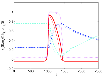
Figure 6: Asymptotic reconstruction of the temporal profiles of $v_{k}(t)$ (thick solid line), $m_{k}$ (thick dotted line), $n_{k}$ (thick dashed-dotted line), $h_{k}$ (thick dashed line), versus the actual temporal profiles (thin lines). All variables are expressed in dimensionless units.

Our construction characterizes the speed of the traveling pulse: it is the speed of the wave front solution of (14)-(15) with $n_{k}\sim n^{*}$ and $h_{k}\sim h^{*}$. The speed of these fronts can be predicted by a depinning analysis for small speeds (as in cbn ) or in terms of continuous waves for large speeds (as in keener1 ).

Let us now compute the width of the pulse. In the peak, $(n_{k},h_{k})$ lies in the integral curve of:

$$\begin{array}[]{l}{dh\over dn}={\lambda\Lambda_{h}\big{(}\nu^{(3)}(n,h)\big{)}\big{[}h_{\infty}\big{(}\nu^{(3)}(n,h)\big{)}-h\big{]}\over\Lambda_{n}\big{(}\nu^{(3)}(n,h)\big{)}\big{[}n_{\infty}\big{(}\nu^{(3)}(n,h)\big{)}-n\big{]}},\end{array}$$ (24)

selected by $h(n^{*})=h^{*}$ and $h(n^{[1]})=n^{[1]}$. Going back to the time scale $t={T\over\epsilon}$ in (19), the peak width is:

$$\begin{array}[]{l}{\cal T}_{1}=\!{T_{1}-T_{0}\over\epsilon}=\!\int_{n^{*}}^{n^{[1]}}\!\!{ds\over\epsilon\Lambda_{n}\big{(}\nu^{(3)}(s,h(s))\big{)}\big{[}n_{\infty}\big{(}\nu^{(3)}(s,h(s))\big{)}-s\big{]}}\end{array}$$ (26)

where the integral is calculated along the solution $h(n)$ of (24). Similarly, the duration of tail is:

$${\cal T}_{2}=\int_{n^{[1]}}^{n^{*}}{ds\over\epsilon\Lambda_{n}\big{(}\nu^{(1)}(s,h(s))\big{)}\big{[}n_{\infty}\big{(}\nu^{(1)}(s,h(s))\big{)}-s\big{]}},$$ (27)

with

$$\begin{array}[]{l}{dh\over dn}={\lambda_{h}\Lambda_{h}\big{(}\nu^{(1)}(n,h)\big{)}\big{[}h_{\infty}\big{(}\nu^{(1)}(n,h)\big{)}-h\big{]}\over\Lambda_{n}\big{(}\nu^{(1)}(n,h)\big{)}\big{[}n_{\infty}\big{(}\nu^{(1)}(n,h)\big{)}-n\big{]}},\;h(n^{[1]})=h^{[1]}.\end{array}$$ (29)

The integral ${\cal T}_{2}$ diverges due to a singularity at $n^{*}$. However, we can use it to predict how long does it take for the tail to get close enough to $n^{*},h^{*}$ replacing $n^{*}$ by $n^{*}-\eta$.

The spatial length of the peak is found using the traveling wave structure: $v_{k}(t)=v(k-ct).$ Thus, ${\cal T}_{1}$ is the time elapsed from the instant at which the leading front reaches a point $k$ to the instant when the end of the peak crosses the same point $k$. The number of nodes $L_{1}$ in the pulse peak is approximately the integer part of:

$$\begin{array}[]{l}L_{1}\sim c_{+}(n^{*},h^{*}){\cal T}_{1}.\end{array}$$ (31)

Our asymptotic construction is consistent when $L_{1}\geq 1$. This yields a restriction on the size of $\epsilon$ for the existence of pulses:

$$\epsilon\leq c_{+}\!\int_{n^{*}}^{n^{[1]}}\!\!{ds\over\Lambda_{n}\big{(}\nu^{(3)}(s,h(s))\big{)}\big{[}n_{\infty}\big{(}\nu^{(3)}(s,h(s))\big{)}-s\big{]}}.$$ (32)

A similar argument can be applied in the infinite tail to quantify the number of nodes at which $n_{k},h_{k}$ depart noticeably from equilibrium.

The values predicted by our asymptotic theory for the parameters in Appendix B are $c=c_{+}=0.069$, $n^{[1]}=0.777$, $h^{[1]}=0.099$, $L_{1}=12$, in good agreement with the numerical measurements. The leading and trailing edges contain about $4$ more nodes, that we have neglected.

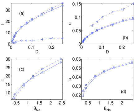
Figure 7: Spatial width of the peak (circles) compared to the predicted width (squares) as a function of: (a) $D$ and (c) $g_{Na}$. In (a), triangles represent the number of additional nodes forming the leading edge; Speed of the pulse (circles) compared to the predicted speed (squares) as a function of: (b) $D$ and (d) $g_{Na}$. In (b), triangles represent the speed of the FHN reduction. All variables are expressed in dimensionless units.

Figure 7 compares the predicted and numerically measured widths and speeds as the parameters $D$ and $g_{Na}$ change. Notice that the values $(n^{*},h^{*})$ and $(n^{[1]},h^{[1]})$ are independent of $D$. Thus, the dependence of the width on $D$ comes through the speed. This explains the similar curves observed in Figure 7 (a) and (b). The triangles in Figure 7 (a) represent the number of nodes in the leading edge, that must be added to compute the total length of a peak. Changes in $g_{Na}$ affect the curves $\nu^{(i)}(n,h)$, $i=1,2,3$, and the speed of the fronts in the reduced fast system. As Figures 7 (c) and (d) show, the quantitative agreement between predicted and numerically measured widths and speeds is reasonable, as long as we are not close to the critical thresholds $D_{c}$ and $\epsilon_{c}$ for propagation failure. We will discuss this point further in Section V.

For the parameters indicated in (74), FHN type reductions perform poorly. The widths predicted as $D$ changes are particularly bad. We find 160 or 250 points in the peak, when 18 or 34 are expected. The predictions for the speed are better, see the triangles in Figure 7 (b). Similar comments apply when $g_{Na}$ is modified.

IV Asymptotic construction of wave trains

When a nerve fiber is periodically excited, we expect propagation of signals in form of wave trains. Wave trains resemble a sequence of identical pulses periodically spaced keener3 . The asymptotic description of each of these pulses is similar to the construction of solitary pulses given in Section III. However, there are several differences. First, the front of the pulses is another pulse and not a region at equilibrium. Second, the leading edge is a wave front solution of the fast reduced system (14)-(15) with $n_{k}=N$, $h_{k}=H$, $(N,H)\neq(n^{*},h^{*})$. This wave front solution selects the speed $c=c_{+}(N,H)$ of the wave train. It has to match the tail of the previous pulse, described by the slow reduced system (19) with $v_{k}=\nu^{(1)}(n_{k},h_{k})$. Thus, we find a family of wave trains for couples $(N,H)$ lying on an integral curve of:

$${dh\over dn}={\lambda\Lambda_{h}(\nu^{(1)}(n,h))\big{[}h_{\infty}(\nu^{(1)}(n,h))-h\big{]}\over\Lambda_{n}(\nu^{(1)}(n,h))\big{[}n_{\infty}(\nu^{(1)}(n,h))-n\big{]}}.$$ (33)

The curve is selected by observing that each pulse in the wave train has one driving leading edge, as in Section III. This means that $h(n^{[1]})=h^{[1]}$, where $(n^{[1]},h^{[1]})$ are the values for which $\nu^{(2)}(n^{[1]},h^{[1]})=\nu^{(3)}(n^{[1]},h^{[1]})$.

The spatial period is approximated by adding the lengths of the smooth regions: $L(N,H)=c_{+}(N,H){\cal T(N,H)}$ where ${\cal T}(N,H)={\cal T}_{1}(N,H)+{\cal T}_{2}(N,H)$ is the time spent in the excited and recovery branches. The temporal lengths ${\cal T}_{1},{\cal T}_{2}$ are defined as in Section III, with $n^{*},h^{*}$ replaced by $N,H$. Now, ${\cal T}_{2}(N,H)$ is finite.

The values predicted by our asymptotic theory for Figure 4 are $c=c_{+}=0.052$, $n^{[1]}=0.755$, $h^{[1]}=0.09$, $L\sim 37-38$, in good agreement with the numerical measurements. Numerically, we obtain $L\sim 43$ for the spatial period. The difference is approximately the number of points in the edges, that we have neglected.

V Propagation failure

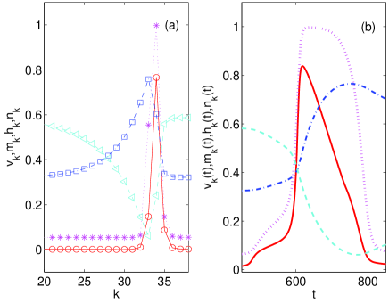
Figure 8: Action potential near propagation failure: (a) Spatial profiles of $v_{k}$ (circles), $m_{k}$ (asterisks), $n_{k}$ (squares) and $h_{k}$ (triangles) superimposed at $t$ fixed, (b) Temporal profiles of $v_{k}(t)$ (solid), $m_{k}(t)$ (dotted), $n_{k}(t)$ (dotted-dashed) and $h_{k}(t)$ (dashed) superimposed for $k$ fixed. All variables are expressed in dimensionless units.

Pulses may fail to propagate at least by two reasons: weak coupling and inadequate time scale separation between the different variables. Weak couplings cause propagation failure by pinning the leading edge of the pulse. A small time scale separation between the two blocks of slow and fast variables produces pulses of vanishing width. Other scenarios for failure might arise when more than two time scales are present. We focus here on mechanisms for failure associated with changes in the parameters due to illness or drugs.

V.1 Propagation failure due to damage in the myelin sheath

The loss of myelin alters the value of the coupling coefficient $D$. Then, the leading wave front can only propagate if the $D$ is large enough to avoid the pinning in the fast reduced system (14)-(15) with $n_{k}=n^{*}$ and $h_{k}=h^{*}$. The critical coupling $D_{c}$ depends on the shape of the nonlinear sources, which is controlled by the parameters $g_{Na}$,$g_{K}$,$g_{L}$, $V_{Na}$,$V_{K}$ and $V_{L}$. The general rule is that the area $A_{23}$ enclosed by $f(v)$ between its second and the third zeroes has to be large enough (depending on $D$) for the leading edge to propagate. The proximity of failure is detected by the fact that the wave profiles develop ‘steps’. Figure 8(b) illustrates generation of ‘steps’ in the time profile of the pulse for $v_{k}$ near propagation failure $D=0.0072\sim D_{c}$. As for bistable equations, the depinning transition is associated with a bifurcation in the system cbn .

V.2 Propagation failure due to the action of chemicals

Many drugs block the propagation of nerve impulses by reducing sodium and potassium conductivities scott1 ; keener2 . Figure 5(b) illustrates the impact of decreasing $g_{Na}$ on the shape of $f$. The enclosed area decreases and so does the propagation speed, up to a critical value at which the width of the pulses (given by formula (31)) vanishes. Only decremental pulses are observed, see Figure 9.

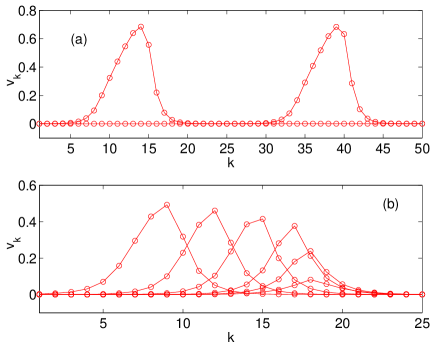
Figure 9: Impact of decreasing $g_{Na}$ on pulse propagation: (a) $g_{Na}=0.745$, (b) $g_{Na}=0.497$. The spatial action potentials have been superimposed at different times. All variables are expressed in dimensionless units.

VI Conclusion

We have introduced an asymptotic strategy to construct solitary pulses and wave trains in the discrete Hodgkin-Huxley model. Unlike FHN reductions, our asymptotic descriptions agree reasonably well with numerical solutions of the discrete HH system. We have discussed two mechanisms for propagation failure. The first one is related to damage in the myelin sheath and is reminiscent of the depinning transitions for wave fronts in bistable systems cbn as the coupling decreases. The second mechanism reflects the impact of chemicals on the time scale separation in the model. Our analysis applies to isolated nerve fibers. However, real motor nerves of vertebrates comprise several hundred of interacting fibers scott2 . It would be interesting to extend our asymptotic predictions to bundles of fibers.

Our asymptotic construction may be useful to understand systems with a mathematical structure similar to HH: models for propagation of impulses through cardiac tissue beeler , models of charge transport in semiconductor superlattices bonilla or the more complex Frankenhauser-Huxley model for myelinated nerves goldman .

Appendix A The discrete Hodgkin-Huxley model for myelinated nerves

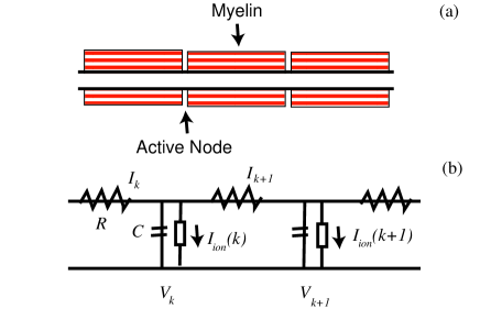
Figure 10: (a) Structure of a myelinated nerve fiber (not to scale). (b) Equivalent circuit for a myelinated nerve fiber.

Myelinated nerve fibers are covered almost everywhere by an insulating coat of myelin. Only at small active sites (nodes of Ranvier) can the membrane function in the normal way. Figure 10(a) illustrates the structure of a myelinated fiber. The length of the myelin sheath is typically $1$ to $2$ $mm$ (close to $100d$ where $d$ is the fiber diameter) and the width of the nodes is about $1\mu m$. The nodes have conduction properties similar to the unmyelinated nerve membrane, while the myelin has a much higher resistance and lower capacitance than the axonal membrane keener2 . Myelinated nerve fibers can be described by a linear diffusion equation which is periodically loaded by the active nodes pickard66 ; markin1967 ; fh . This picture can be simplified by lumping the internode capacitance of the myelin together with the nodal capacitance scott1 . The myelin is considered to be a perfect insulator. This leads to the equivalent circuit in Figure 10(b). $C$ and $R$ represent lumped resistance and capacitance. $V_{k}$, $I_{k}$ and $I_{ion}(k)$ represent the membrane potential, internodal current and ionic current at the $k$-th node. Applying Kirchoff’s laws to the circuit yields:

$$V_{k-1}-V_{k}=RI_{k},\quad I_{k}-I_{k+1}=C{dV_{k}\over dt}+I_{ion}(k)$$ (34)

Adopting at each node the Hodgkin-Huxley expression for the ion current hh , we obtain the discrete Hodgkin-Huxley model for a myelinated axon:

$$\begin{array}[]{l}C{dV_{k}\over dT}+I_{ion}(V_{k},M_{k},N_{k},H_{k})=\\ \overline{D}(V_{k+1}-2V_{k}+V_{k-1}),\end{array}$$ (37)

$$\begin{array}[]{l}{dM_{k}\over dT}=\overline{\lambda}_{M}\overline{\Lambda}_{M}(V_{k})(M_{\infty}(V_{k})-M_{k}),\\ {dN_{k}\over dT}=\overline{\lambda}_{N}\overline{\Lambda}_{N}(V_{k})(N_{\infty}(V_{k})-N_{k}),\\ {dH_{k}\over dT}=\overline{\lambda}_{H}\overline{\Lambda}_{H}(V_{k})(H_{\infty}(V_{k})-H_{k}),\end{array}$$ (41)

where the index $k$ designs the $k$-th node of the fiber. Here, $V_{k}$ is the deviation from rest of the membrane potential, $N_{k}$ is the potassium activation, $M_{k}$ is the sodium activation and $H_{k}$ the sodium inactivation. The ion current is given by:

$$\begin{array}[]{l}I_{ion}(V,M,N,H)=\overline{g}_{Na}M^{3}H(V-\overline{V}_{Na,R})\\ +\overline{g}_{L}(V-\overline{V}_{L,R})+\overline{g}_{K}N^{4}(V-\overline{V}_{K,R}).\\ \end{array}$$ (44)

The fraction of open $K^{+}$ channels is computed as $N_{k}^{4}$. The fraction of open $Na^{+}$ channels is approximated by $M_{k}^{3}H_{k}$. The parameters have the following interpretation. $\overline{g}_{Na}$ and $\overline{g}_{K}$ are the maximum conductance values for $Na^{+}$ and $K^{+}$ pathways, respectively. $\overline{g}_{L}$ is a constant leakage conductance. The corresponding equilibrium potentials are $\overline{V}_{Na}$, $\overline{V}_{K}$ and $\overline{V}_{L}$, respectively. Then, $\overline{V}_{Na,R}=\overline{V}_{Na}-\overline{V}_{R}$, $\overline{V}_{K,R}=\overline{V}_{K}-\overline{V}_{R}$ and $\overline{V}_{L,R}=\overline{V}_{L}-\overline{V}_{R},$ where $\overline{V}_{R}$ is the resting potential. $C$ is the membrane capacitance. The coefficient $\overline{D}={1\over L(r_{i}+r_{e})}={1\over R}$, where $L$ is the length of the myelin sheath between nodes and $r_{i},r_{e}$ the resistances per unit length of intracellular and extra-cellular media.

This model is adequate for the long axons of peripheral myelinated nerves. More biological detail can be included by adding an equation for the membrane potential $V(x,t)$ across the myelin sheath in the internodes fh :

$$c{\partial V\over\partial T}={1\over r_{i}+r_{e}}{\partial^{2}V\over\partial^{2}x}-{V\over r},\quad x\in(x_{k},x_{k+1}),t>0$$ (45)

$$V(x_{k},t)=V_{k}(t),\;V(x_{k+1},t)=V_{k+1}(t)$$ (46)

coupled with (41) and:

$$C{dV_{k}\over dT}+I_{ion}(V_{k},M_{k},N_{k},H_{k})=I_{k}(t),$$ (47)

$$I_{k}(t)={1\over r_{i}+r_{e}}[{\partial V\over\partial x}(x_{k}^{+},t)-{\partial V\over\partial x}(x_{k}^{-},t)].$$ (48)

This model produces a good quantitative approximation of the conduction velocity for toad axons fh . Numerical simulations of the sensitivity to different parameters (diameter, nodal area…) produce results in agreement with experiments moore78 ; goldman . The discrete model (37)-(41) is recovered by assuming that the axial currents along the myelin sheath ${\partial V\over\partial x}(x,t)$ are constant in each internode. Then, ${\partial V\over\partial x}(x,t)={V_{k+1}(t)-V_{k}(t)\over L}$ in $[x_{k},x_{k+1}]$ with $L=x_{k+1}-x_{k}$. As a result, $I_{k}(t)={1\over L(r_{i}+r_{e})}(V_{k+1}-V_{k}+V_{k-1})$. This approximation is reasonable in view of the numerical results in fh (see Figure 2 therein).

Appendix B Dimensionless equations

For our numerical tests we have selected the parameters and coefficient functions of a frog. For the motor nerve of a frog, the data in cole can be fitted by the following rate and stationary state functions:

$$\begin{array}[]{l}\overline{\Lambda}_{M}(V)\!=\!0.03\big{[}{2.5-0.1V\over\exp(2.5-0.1V)-1}+4\;\exp({-V\over 18})\big{]},\\ M_{\infty}(V)\!=\!\big{[}1+4\exp({-V\over 18}){\exp(2.5-0.1V)-1\over(2.5-0.1V)}\big{]}^{-1},\\ \overline{\Lambda}_{H}(V)\!=\!\big{[}0.07\exp({-V\over 20})+{1\over\exp(3-0.1V)+1}\big{]},\\ H_{\infty}(V)\!=\!\big{[}1+{\exp({V\over 20})\over 0.07\big{(}\exp(3-0.1V)+1\big{)}}\big{]}^{-1},\\ \overline{\Lambda}_{N}(V)\!=\!0.79\big{[}{0.1-0.01V\over\exp(1-0.1V)-1}+0.125\;\exp({-V\over 80})\big{]},\\ N_{\infty}(V)\!=\!\big{[}1+0.125\exp({-V\over 80}){\exp(3-0.1V)-1\over(0.1-0.01V)}\big{]}^{-1}.\end{array}$$ (55)

Typical values of the parameters cole ; scott1 are given below:

$$\begin{array}[]{|c|c|c|c|}\hline\cr\overline{D}&\overline{g}_{Na}&\overline{g}_{K}&\overline{g}_{L}\\ \hline\cr 1/28(M\Omega)^{-1}&0.57\;\mu mho&0.104\;\mu mho&0.025\;\mu mho\\ \hline\cr\overline{V}_{R}&\overline{V}_{Na}&\overline{V}_{K}&\overline{V}_{L}\\ \hline\cr-75\;mV&47\;mV&-75\;mV&-75\;mV\\ \hline\cr C&\overline{\lambda}_{M}&\overline{\lambda}_{H}&\overline{\lambda}_{N}\\ \hline\cr 2.6-4.7\;pF&127\;(ms)^{-1}&1.76\;(ms)^{-1}&2\;(ms)^{-1}\\ \hline\cr\end{array}$$ (62)

We nondimensionalize the model by choosing as new variables $v_{k}={V_{k}\over\overline{V}_{Na,R}}$, $t=T\overline{\lambda}_{M}$, $m_{k}=M_{k}$, $n_{k}=N_{k}$, $h_{k}=H_{k}$. The dimensionless equations are:

$$\begin{array}[]{l}{dv_{k}\over dt}+g_{K}n_{k}^{4}(v_{k}-{V}_{K})+{g}_{Na}m_{k}^{3}h_{k}(v_{k}-1)+\\ {g}_{L}(v_{k}-{V}_{L})=D(v_{k+1}-2v_{k}+v_{k-1}),\\ {dm_{k}\over dt}=\Lambda_{m}(v_{k})\big{[}m_{\infty}(v_{k})-m_{k}\big{]},\\ {dn_{k}\over dt}=\lambda_{n}\Lambda_{n}(v_{k})\big{[}n_{\infty}(v_{k})-n_{k}\big{]},\\ {dh_{k}\over dt}=\lambda_{h}\Lambda_{h}(v_{k})\big{[}h_{\infty}(v_{k})-h_{k}\big{]}.\end{array}$$ (68)

Set $G=C\overline{\lambda}_{M}$. Then, the dimensionless parameters are given by:

$$\begin{array}[]{|c|c|c|c|c|c|c|c|c|}\hline\cr{g}_{Na}&{g}_{K}&{g}_{L}&D&{V}_{K}&{V}_{L}&\lambda_{n}&{\lambda}_{m}\\ \hline\cr{\overline{g}_{Na}\over G}&{\overline{g}_{K}\over G}&{\overline{g}_{L}\over G}&{\overline{D}\over G}&{\overline{V}_{K,R}\over\overline{V}_{Na,R}}&{\overline{V}_{L,R}\over\overline{V}_{Na,R}}&{\overline{\lambda}_{N}\over\overline{\lambda}_{M}}&{\overline{\lambda}_{H}\over\overline{\lambda}_{M}}\\ \hline\cr\end{array}$$ (71)

The new rate functions and stationary states are obtained from (55) replacing $V$ by $v\overline{V}_{Na,R}$. In dimensionless units, the parameters for a frog nerve become:

$$\begin{array}[]{|c|c|c|c|c|c|c|c|}\hline\cr{D}&{g}_{Na}&{g}_{K}&{g}_{L}&{V}_{K}&{V}_{L}&{\lambda}_{h}&{\lambda}_{n}\\ \hline\cr 0.093&1.49&0.27&0.065&0&0&0.014&0.015\\ \hline\cr\end{array}$$ (74)

In our asymptotic analysis, we choose $\lambda_{n}=\epsilon$ as small parameter and write $\lambda_{h}=\epsilon\lambda$, $\lambda={\lambda_{h}\over\lambda_{n}}\sim 1$.

Appendix C Equations for the wave profiles

The wave profiles and speeds solve an eigenvalue problem for a system of differential-difference equations:

$$\begin{array}[]{lll}-cv_{z}(z)&=&D(v(z+1)-2v(z)+v(z-1))\\ &&-I(v(z),m(z),n(z),h(z)),\\ -cm_{z}(z)&=&\Lambda_{m}(v(z))\big{[}m_{\infty}(v(z))-m(z)\big{]},\\ -cn_{z}(z)&=&\epsilon\Lambda_{n}(v(z))\big{[}n_{\infty}(v(z))-n(z)\big{]},\\ -ch_{z}(z)&=&\epsilon\lambda\Lambda_{h}(v(z))\big{[}h_{\infty}(v(z))-h(z)\big{]}.\end{array}$$ (80)

In a solitary pulse, the profiles tend to the equilibrium states as $z\rightarrow\pm\infty$. In a wave train, the profiles are periodic: $v(z)=v(z+L)$, $m(z)=m(z+L)$, $n(z)=n(z+L)$ and $h(z)=h(z+L)$, $L$ being the spatial period.

Appendix D Reconstruction of the temporal profile

We describe below the matching conditions and the uniform reconstruction of the pulse profiles in the different regions. The superscripts (I),…,(V) refer to the reduced descriptions corresponding to regions (1),…,(5). We have:

• The matching conditions for the reduced descriptions of the front of the pulse and the leading edge at $T=T_{0}$ are:

  $$\begin{array}[]{l}v^{*}-v_{k}^{(II)}({T-T_{1}\over\epsilon})\ll 1,\;m^{*}-m_{k}^{(II)}({T-T_{1}\over\epsilon})\ll 1,\\ \end{array}$$ (82)

  if $\epsilon\ll T_{0}-T\ll 1$. The uniform approximations of the profiles for $T\leq T_{0}$ are:

  $$\begin{array}[]{ll}v_{k}^{unif}=&v_{k}^{(II)}({T-T_{0}\over\epsilon}),\quad n_{k}^{unif}=n^{*},\\ m_{k}^{unif}=&m_{k}^{(II)}({T-T_{0}\over\epsilon}),\quad h_{k}^{unif}=h^{*}.\end{array}$$ (85)

• The matching conditions for the reduced descriptions of the peak of the pulse and the leading edge at $T=T_{0}$ are:

  $$\begin{array}[]{l}\nu^{(3)}_{1}(n_{k}^{(III)}(T),h_{k}^{(III)}(T))-v_{k}^{(II)}({T-T_{0}\over\epsilon})\ll 1,\\ m_{\infty}\big{(}\nu^{(3)}_{1}(n_{k}^{(III)}(T),h_{k}^{(III)}(T))\big{)}-m_{k}^{(II)}({T-T_{0}\over\epsilon})\ll 1,\\ n_{k}^{(III)}(T)-n^{*}\ll 1,\;h_{k}^{(III)}(T)-h^{*}\ll 1,\end{array}$$ (89)

  if $\epsilon\ll T-T_{0}\ll 1$. The uniform approximations of the profiles in regions (II)-(III) are:

  $$\begin{array}[]{ll}v_{k}^{unif}=&v_{k}^{(II)}({T-T_{0}\over\epsilon})+\nu^{(3)}_{1}(n_{k}^{(III)}(T),h_{k}^{(III)}(T))\\ &-\nu^{(3)}_{1}(n^{*},h^{*}),\\ m_{k}^{unif}=&m_{k}^{(II)}({T-T_{0}\over\epsilon})+m_{\infty}\big{(}\nu^{(3)}_{1}(n_{k}^{(III)}(T),h_{k}^{(III)}(T))\big{)}\\ &-m_{\infty}\big{(}\nu^{(3)}_{1}(n^{*},h^{*})\big{)},\\ n_{k}^{unif}=&n_{k}^{(III)}(T),\;h_{k}^{unif}=h_{k}^{(III)}(T).\end{array}$$ (95)

• The matching conditions for the reduced descriptions of the peak of the pulse and the trailing edge at $T=T_{1}$ are:

  $$\begin{array}[]{l}\nu^{(3)}_{1}(n_{k}^{(III)}(T),h_{k}^{(III)}(T))-v_{k}^{(IV)}({T-T_{1}\over\epsilon})\ll 1,\\ m_{\infty}\big{(}\nu^{(3)}_{1}(n_{k}^{(III)}(T),h_{k}^{(III)}(T))\big{)}-m_{k}^{(IV)}({T-T_{1}\over\epsilon})\ll 1,\\ n_{k}^{(II)}(T)-n^{*}\ll 1,\;h_{k}^{(II)}(T)-h^{*}\ll 1,\end{array}$$ (99)

  if $\epsilon\ll T_{1}-T\ll 1$. The uniform approximations of the profiles in regions (II)-(III)-(IV) are:

  $$\begin{array}[]{ll}v_{k}^{unif}=&v_{k}^{(II)}({T-T_{0}\over\epsilon})+v_{k}^{(IV)}({T-T_{1}\over\epsilon})\\ &+\nu^{(3)}_{1}(n_{k}^{(III)}(T),h_{k}^{(III)}(T))\\ &-\nu^{(3)}_{1}(n^{*},h^{*})-\nu^{(3)}_{1}(n^{[1]},h^{[1]}),\\ m_{k}^{unif}=&m_{k}^{(II)}({T-T_{0}\over\epsilon})+m_{k}^{(IV)}({T-T_{1}\over\epsilon})\\ &+m_{\infty}\big{(}\nu^{(3)}_{1}(n_{k}^{(III)}(T),h_{k}^{(III)}(T))\big{)}\\ &-m_{\infty}\big{(}\nu^{(3)}_{1}(n^{*},h^{*})\big{)}-m_{\infty}\big{(}\nu^{(3)}_{1}(n^{[1]},h^{[1]})\big{)},\\ n_{k}^{unif}=&n_{k}^{(III)}(T),\;h_{k}^{unif}=h_{k}^{(III)}(T).\end{array}$$ (107)

• The matching conditions for the reduced descriptions of the tail of the pulse and the trailing edge at $T=T_{1}$ are:

  $$\begin{array}[]{l}\nu^{(1)}_{1}(n_{k}^{(V)}(T),h_{k}^{(V)}(T))-v_{k}^{(IV)}({T-T_{1}\over\epsilon})\ll 1,\\ m_{\infty}\big{(}\nu^{(1)}_{1}(n_{k}^{(V)}(T),h_{k}^{(V)}(T))\big{)}-m_{k}^{(IV)}({T-T_{1}\over\epsilon})\ll 1,\\ n_{k}^{(V)}(T)-n^{*}\ll 1,\;h_{k}^{(V)}(T)-h^{*}\ll 1,\end{array}$$ (111)

  if $\epsilon\ll T-T_{1}\ll 1$. The uniform approximations of the profiles for $T\geq T_{1}$ are:

  $$\begin{array}[]{ll}v_{k}^{unif}=&v_{k}^{(IV)}({T-T_{1}\over\epsilon})+\nu^{(1)}_{1}(n_{k}^{(V)}(T),h_{k}^{(V)}(T))\\ &-\nu^{(1)}_{1}(n^{[1]},h^{[1]}),\\ m_{k}^{unif}=&m_{k}^{(IV)}({T-T_{1}\over\epsilon})+m_{\infty}\big{(}\nu^{(1)}_{1}(n_{k}^{(V)}(T),h_{k}^{(V)}(T))\big{)}\\ &-m_{\infty}\big{(}\nu^{(1)}_{1}(n^{[1]},h^{[1]})\big{)},\\ n_{k}^{unif}=&n_{k}^{(V)}(T),\;h_{k}^{unif}=h_{k}^{(V)}(T).\end{array}$$ (117)

Appendix E Pulses formed by two wavefronts

For the choice of parameters indicated in (74), the third region of the pulse ends when two branches of roots of the cubic source collapse. For other parameters, the situation might be different. It might happen that along the integral curve (24) we find a couple $(n^{[1]},h^{[1]})$ such that there are wave front solutions of the reduced fast system traveling with speed $c_{-}(n^{[1]},h^{[1]})=c_{+}(n^{*},h^{*})$. Then, the top of the pulse ends at this point and the fourth region is now a traveling wave front. The pulse is formed by two rigidly moving traveling wave fronts.

Whether a traveling wave front is formed in the back of the pulse or not, can be guessed from the shape of the nonlinear source $f$. Figure 5(a) depicts $f(v;n,h)$ with the parameters values (74) when $(n,h)=(n^{*},h^{*})$. It is strongly asymmetric. The magnitude of the speed of the leading wave front is intuitively related to size of the area enclosed by $f(v;n^{*},h^{*})$ between its second and third zeroes, $A^{*}$. If we vary $(n,h)$ along the curve (24), the speed of a back front is related to the area $A$ enclosed by $f(v;n,h)$ between its first and the second zeroes. We find that such areas are always smaller than $A^{*}$ and the cubic structure is finally lost. A trailing wave front moving at the same speed as the leading wave front cannot be formed. Back wave fronts can only be observed for more symmetrical sources, when varying $(n,h)$ along the curve (24) we can make $A$ equal to $A^{*}$.

We describe here how to modify the asymptotic construction in Sections III and IV to account for pulses formed by two rigidly moving wave fronts. In the asymptotic description of these pulses we distinguish again five regions. The first three are similar:

• The front of the pulse is described by $v_{k}\sim v^{*}$, $m_{k}\sim m^{*}$, $n_{k}\sim n^{*}$ and $h_{k}\sim h^{*}$.

• The leading edge of the pulse is a wave front solution of the fast reduced system (14)-(15) with $n_{k}=n^{*}$ and $h_{k}=h^{*}$ joining $(\nu^{(1)}(n^{*},h^{*}),m_{\infty}(v^{*}))=(v^{*},m^{*})$ and $(\nu^{(3)}(n^{*},h^{*}),m_{\infty}(\nu^{(3)}(n^{*},h^{*}))$. This front propagates with a definite speed $c=c_{+}(n^{*},h^{*})$.

• In the transition between interfaces, $v_{k}=\nu^{(3)}(n_{k},h_{k})$, $m_{k}=m_{\infty}(v_{k})$ and $n_{k},h_{k}$ solve the slow reduced system (19), evolving from $(n^{*},h^{*})$ to $(n^{[1]},h^{[1]})$.

The fourth region is different:

• The trailing edge is the wave front solution for the fast reduced system (14)-(15) with $n_{k}=n^{[1]}$ and $h_{k}=h^{[1]}$, joining $(\nu^{(3)}(n^{[1]},h^{[1]}),m_{\infty}(\nu^{(3)}(n^{[1]},h^{[1]}))$ and $(\nu^{(1)}(n^{[1]},h^{[1]}),m_{\infty}(\nu^{(1)}(n^{[1]},h^{[1]}))$, respectively. $n^{[1]}$ and $h^{[1]}$ are now selected in such a way that this front travels with speed $c=c_{-}(n^{[1]},h^{[1]})=c_{+}(n^{*},h^{*})$.

The fifth is similar:

• In the pulse tail, $v_{k}=\nu^{(1)}(n_{k},h_{k})$, $m_{k}=m_{\infty}(v_{k})$ and $n_{k},h_{k}$ solve the slow reduced system (19), evolving from $(n^{[1]},h^{[1]})$ to $(n^{*},h^{*})$ as $t\rightarrow\infty$.

The temporal and spatial width of the peak can be computed as in Section III. Now, the number of points in the leading and trailing wave fronts are neglected.

For wave trains, the construction in Section IV has to be modified as follows: $(N,H)$ and $(n^{[1]},h^{[1]})$ must lie in the same integral curve of (33) and satisfy $c=c_{-}(n^{[1]},h^{[1]})=c_{+}(N,H)$.

References

- (1) E-address ana-carpio@mat.ucm.es.
- (2) A.R.A. Anderson and B.D. Sleeman, Int. J. Bif. Chaos, 5, 63 (1995).
- (3) A. Carpio, L.L. Bonilla, SIAM J. Appl. Math., 63 (2), 619, (2002).
- (4) J.P. Keener, SIAM J. Appl. Math., 47, 556 (1987).
- (5) G. Fáth, Physica D, 116, 176 (1998).
- (6) A. Carpio, L.L. Bonilla, Phys. Rev. Lett, 86, 6034, (2001).
- (7) J.J. Struijk, Biophys. J., 72, 2457 (1997).
- (8) W.A.H. Rushton, J. Physiol., London, 115, 101 (1951).
- (9) A. C. Scott, Rev. Modern Phys., 47, 487 (1975); A.C. Scott, Neuroscience, Springer, Berlin, 2002.
- (10) S. Pluchino, A. Quattrini, E. Brambilla et al, Nature 422, 688 (2003).
- (11) J.P. Keener, J. Sneyd, Mathematical Physiology, Springer, New York, 1998, Chapters 4 and 9.
- (12) H. Kunov, Proc. IEEE, 55 (1967) 427-428.
- (13) V. Booth, T. Erneux, SIAM J. Appl. Math., 55, 1372 (1995).
- (14) X. Chen, S.P. Hastings, J. Math. Biol., 38, 1 (1999).
- (15) A. Tonnelier, Phys. Rev. E, 67, 036105, (2003).
- (16) I. Richer, IEEE Trans. Circuit Theory, CT-13, 388 (1996).
- (17) B. Zinner, J. Diff. Eq., 96, 1 (1992).
- (18) T. Erneux, G. Nicolis, Physica D, 67, 237 (1993).
- (19) R. FitzHugh, Biophys. J., 2, 11 (1962).
- (20) L. Goldman, J.S. Albus, Biophys. J., 8 596 (1968).
- (21) J.W. Moore, R.W. Joyner, M.H. Brill, S.D. Waxman, M. Najar-Joa, Biophys. J., 21, 147, (1978).
- (22) C.B. Muratov, Biophys. J., 79, 2893, (2000).
- (23) R. FitzHugh, Biophys. J., 1, 445 (1961); J. Nagumo, S. Arimoto, S. Yoshizawa, Proc. Inst. Radio Engineers, 50, 2061 (1962).
- (24) P. A. Lagerstrom, Matched asymptotic expansions. Springer, N. Y. 1988.
- (25) In fact, stages (3)-(5) can be considered as one region described by the reduced system of four ordinary differential equations obtained setting . The three regions arise by further reducing the system using the splitting between fast and slow variables.
- (26) J.P. Keener, SIAM J. Appl. Math., 39, 528, (1980).
- (27) S. Binczak, J.C. Eilbeck, A.C. Scott, Physica D, 148, 174 (2001).
- (28) G.W. Beeler, H.J. Reuter, J. Physiol., 268, 177, (1977).
- (29) L.L. Bonilla, H.T. Grahn, Rep. Prog. Phys., 68, 577-683, (2005).
- (30) W.F. Pickard, J. Theoret. Biol., 11, 30, (1966).
- (31) V.S. Markin, Yu. A. Chimadzhev, Biophys. J., 12, 1032, (1967).
- (32) A.L. Hodgkin, A.F. Huxley, J. Physiol., London, 117, 500 (1952).
- (33) K. S. Cole, Membranes, ions and impulses, Univ. Calif. Press, Berkeley, 1968.