The contact network of patients in a regional healthcare system

Abstract

Yet in spite of advances in hospital treatment, hospitals continue to be a breeding ground for several airborne diseases and for diseases that are transmitted through close contacts like SARS, methicillin-resistant Staphylococcus aureus (MRSA), norovirus infections and tuberculosis (TB). Here we extract contact networks for up to 295,108 inpatients for durations up to two years from a database used for administrating a local public healthcare system serving a population of 1.9 million individuals. Structural and dynamical properties of the network of importance for the transmission of contagious diseases are then analyzed by methods from network epidemiology. The contact networks are found to be very much determined by an extreme (age independent) variation in duration of hospital stays and the hospital structure. We find that that the structure of contacts between in-patients exhibit structural properties, such as a high level of transitivity mejn:clu , assortativity mejn:ass and variation in number of contacts and:may , that are likely to be of importance for the transmission of less contagious diseases. If these properties are considered when designing prevention programs the risk for and the effect of epidemic outbreaks may be decreased.

I Limitations of traditional epidemiology

A central parameter within infection epidemiology is the basic reproduction number $R_{0}$ and:may . $R_{0}$ is used to estimate whether a disease is contagious enough to generate an epidemic in a specific population. In its simplest form, is defined as the expected number of individuals that an infected individual will infect in a completely susceptible population. If all individuals in a population have approximately the same number of contacts, and the probability that any pair of individuals will meet is equal, $R_{0}$ can be estimated by the function below:

$$R_{0}=c\beta D,$$ (1)

where $c$ stands for umber of contacts per time unit, $\beta$ or likelihood of passing on an infection per contact, and $D$ for the average time an individual is infectious (measured in same time unit as $c$). To make an epidemic possible, the infected person must infect more than one person on average. The threshold value for epidemics is therefore $R_{0}=1$.

Studies have shown that $R_{0}$ in its simplest form may yield misleading results. Anderson and May have demonstrated that a great variation in number of contacts may compensate for a low average number of contacts and:may . This is because individuals with many contacts have a far greater probability of becoming infected, and of passing on an infection. Therefore, in populations with great variation in number of contacts, $R_{0}$ should be calculated as:

$$R_{0}=c\beta D\left(1+\frac{\sigma^{2}}{c^{2}}\right)$$ (2)

where $\sigma^{2}$ denotes the variance in the number of contacts. Another reason that $R_{0}$ can be an oversimplification is that most contact networks studied are known to differ significantly from random interaction.

II Network structure and disease dynamics

Many contact networks are characterized by a high level of transitivity; that is, the number of triangles in the network is much larger than is found in an average network having the same frequency distribution of number of contacts watts . A large clustering coefficient tends to slow down epidemics because the probability that an infected person’s contacts will already be infected is very high in such a network colg ; szen . A common way to estimate clustering in a network is to estimate its relative number of triangles, or more exactly, to calculate the fraction $C$ of all paths of length three in the network which form a triangle:

$$C=\frac{3n_{\mathrm{triangle}}}{n_{\mathrm{triple}}}$$ (3)

where $n_{\mathrm{triangle}}$ is the number of triangles (fully connected subgraphs of three vertices) and $n_{\mathrm{triple}}$ is the number of triples of vertices connected by two or three contacts. The factor three is needed to normalize $C$ to the interval $[0,1]$.

Another difference between contact and random networks is that most contact networks are assortative by number of contacts mejn:ass . This means that individuals who have many contacts tend to have contact with other individuals who also have many contacts, and vice versa. The number of contacts is usually referred to as “degree” in network theory, and we will use this term here. High assortativity decreases the epidemic threshold value among individuals who have many contacts. The standard measure is the assortative mixing coefficient $r$; that is, the symmetric correlation coefficient between the individuals’ degrees on each side of all contacts:

$$r=\frac{4\langle k_{1}k_{2}\rangle-\langle k_{1}+k_{2}\rangle^{2}}{2\langle k_{1}^{2}+k_{2}^{2}\rangle-\langle k_{1}+k_{2}\rangle^{2}}$$ (4)

where $k_{i}$ is the degree of the $i$th argument in a list of the contacts mejn:ass .

III Contact networks of patients

We will now construct networks generated from a unique database consisting of 295,108 individuals who were registered as “in-patients” at any hospital in Stockholm county (pop. 1.8 million) during 2001 and 2002.

We want a contact to represent closeness in space and time. Our spatial requirement is that two patients should be on the same ward. For the temporal aspect we let closeness be a network parameter, and we regard a contact between patients as established if they were hospitalized on the same ward for a duration $t_{\mathrm{ol}}$ (overlap time) or longer. A $t_{\mathrm{ol}}=0$ means that contacts between one patient who was admitted the same day as another patient was discharged are included. Furthermore, we let the sampling time window size $\Delta t$ be another parameter. The two parameters $t_{\mathrm{ol}}$ and $\Delta t$ yield different networks that are relevant to different diseases. For example, for diseases such as measles, SARS, and norovirus, which spread rapidly, a narrow time window will be appropriate hey ; for diseases requiring prolonged contact for transmission, like tuberculosis, the relevant network is represented by a larger $t_{\mathrm{ol}}$.

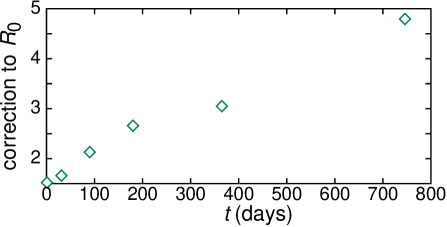
Figure 1: The degree distribution and its effect on the reproduction number. In the upper panel we see the probability density function $P(k)$ versus $k$ (with logarithmic binning) for networks with overlap $t_{\mathrm{ol}}=0$ and different time windows. The lower panel shows the correction to the basic reproduction number $R_{0}$ as a function of the time window size for $t_{\mathrm{ol}}=0$. For example, for $\Delta t=2$ years an epidemic can occur by a disease five times less transmissible than predicted by traditional models.

IV Network structural properties

IV.1 Degree distribution

We will start by plotting the probability density function $P(k)$ for an individual to have $k$ contacts. This function is plotted for, respectively:

• One weekday in January.

• The entire month of January.

• The first six months of 2001.

• The whole period 2001-2002.

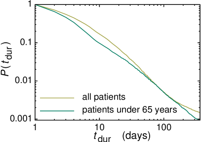
Figure 2: The probability that any hospitalization lasts $\Delta t$ or longer. In A, all data are used; in B, the patients over 60 years are removed from the data set.

In Figure 1A we see the development of this contact structure from an exponential distribution to a degree distribution with a truncated “fat tail.” It is clear that variation in the number of contacts between individuals increases with time. Figure 1B shows the degree to which calculated using Equation 1 must be compensated according to Equation 2 for this increase in variation. The skewed degree distribution in our case is related to the power-law-like distribution of hospitalization times (see Figure 2 and Sect. B). The distribution of hospitalization will indirectly lead to “preferential attachment” ba:model ; klemm (that is, a heightened probability of high-degree vertices to form additional contacts)—a well known mechanism for producing fat-tailed degree distributions price .

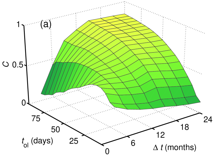
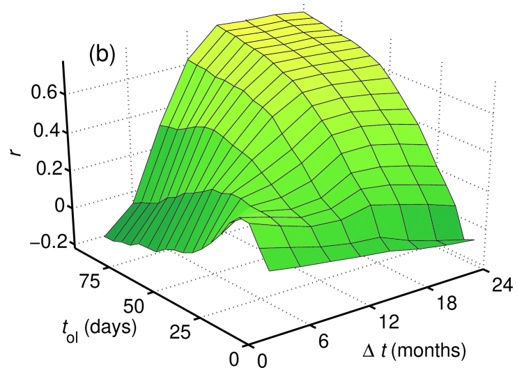
Figure 3: The clustering (A) and assortative mixing (B) coefficients, $C$ and $r$, as functions of sampling time, $\Delta t$, and overlap time, $t_{\mathrm{ol}}$.

IV.2 Transitivity and assortativity

We will now investigate how transitivity, $C$, and assortativity, $r$, vary with sampling time, $\Delta t$, and overlap time, $t_{\mathrm{ol}}$.

In Figure 3(A) we display the clustering coefficient, $C$, and in Figure 3(B) the level of assortative mixing, $r$, as functions of our time intervals $t_{\mathrm{ol}}$ and $\Delta t$. We note that both parameters exhibit a very similar functional form. $C$ and $r$ both decrease with $\Delta t$ when is held constant for small $t_{\mathrm{ol}}$, butincrease when tol is held constant for large values of $t_{\mathrm{ol}}$. Both parameters behave in a similar way when $\Delta t$ is held constant. For small values of $t_{\mathrm{ol}}$, the parameters first increase and then start to decrease as a function of $t_{\mathrm{ol}}$. For large values of $t_{\mathrm{ol}}$, both parameters first increase with $t_{\mathrm{ol}}$ until they converge at a high level of clustering and assortativity.

The estimated high levels for the $C$ and the $r$ parameters, and the resemblance in functional form between the $r$-surface and the $C$-surface in Figure 3 are a consequence of the compartmental structure of the healthcare system. Assume a hypothetical network, $\Omega$ in which all inpatients stay on the same ward during the entire duration of $\Delta t$. In such a network, each inpatient will have a link to each other inpatient on the same ward. The level of clustering between the inpatients will therefore equal 1, both locally on each ward and globally throughout the whole healthcare system, because no links exist between inpatients on different wards in $\Omega$. It is trivial that the level of assortativity can only be defined if there is a variation in ward size, and that $r$ in these cases must equal 1 because the degree of contacts on each side of each link will be equal. Our results show that networks defined by a large value of $t_{\mathrm{ol}}$ and a large value of $\Delta t$ come very close to $\Omega$. Both $C$ and $r$ are large, and the vast majority of individuals in these networks are registered as inpatients only once per ward (see supplementary material). If we relax the restrictions on $\Omega$ such that each inpatient stays on the same ward during the entire period of $\Delta t$, the $C$ and $r$ parameters may drop below 1. This makes it possible for triples, which not are triangles, to be formed between inpatients that stay on different wards, and between inpatients that stay on the same wards but at different times. This also makes it possible for links to form between nodes with different degrees. The same occurs where $\Delta t$ increases when $t_{\mathrm{ol}}$ is held constant for low levels of $t_{\mathrm{ol}}$. The decay in $C$ and $r$ is a result of the skew distribution of hospitalization times (Fig. 2)—a long-term patient A will form a triple (but not a triangle) with the many pairs of short-term patients whose hospitalization does not overlap with each other’s but does overlap with A. This situation, and the number of inpatients who stay on more than one ward, will be more common for larger time windows, causing $C$, and consequently $r$, to decay over time.

That C increases with $t_{\mathrm{ol}}$ (for fixed $\Delta t$) may seem counterintuitive: As $t_{\mathrm{ol}}$ grows, the network will have fewer edges, and also fewer triangles. We have constructed a simple agent-based model that shows that a prerequisite for this is the observed skewed distribution of hospital stays (see Sect. C).

V Summary and conclusions

Our study of a very large inpatient database shows that hospital systems characteristically have a very large variation in duration of hospital stays, which generates a correspondingly large variation in number of contacts. We have further shown that the clustering coefficient and assortative mixing depend greatly on sampling time and the length of time that two inpatients must spend together for contact to be effected. Both of these coefficients, $C$ and $r$, become extremely large in our real-life network when $t_{\mathrm{ol}}$ and $\Delta t$ are large. This is alarming because it has been shown that both a high level of clustering and a high level of assortative interaction decrease the epidemic threshold mejn:clu ; mejn:ass . Any strategy to intervene with disease spread in a hospital environment must take into account this departure from assumptions of random interaction and homogenous mixing. For infections with high transmissibility, short incubation times and short duration of infectiousness, such as norovirus infections and SARS, our finding may be less important. However, for diseases such as tuberculosis or MRSA characterized by low transmissibility and long duration of infectiousness, it becomes necessary to take this variation into consideration because a high variance will lower the epidemic threshold.

Our findings indicate that the individuals with many contacts are significant for the spread of infectious diseases with long duration of infectiousness. These high-risk individuals will probably be identifiable through hospital patient registration systems, and should be the first to be targeted by contact tracing. The high level of clustering further indicates that it may be worth screening all inpatients that have spent time on the same ward as positive inpatients before and after the positive inpatients were there. The high level of clustering makes it reasonable to assume that more than one inpatient will be infectious at the same time on the same ward, and consequently that the disease would have existed among the inpatients on the ward both before and after the actual inpatient in question was on the ward.

Figure 4: Mean duration of hospital stay for the inpatients for each ward versus number of inpatients a year for the wards in the database.

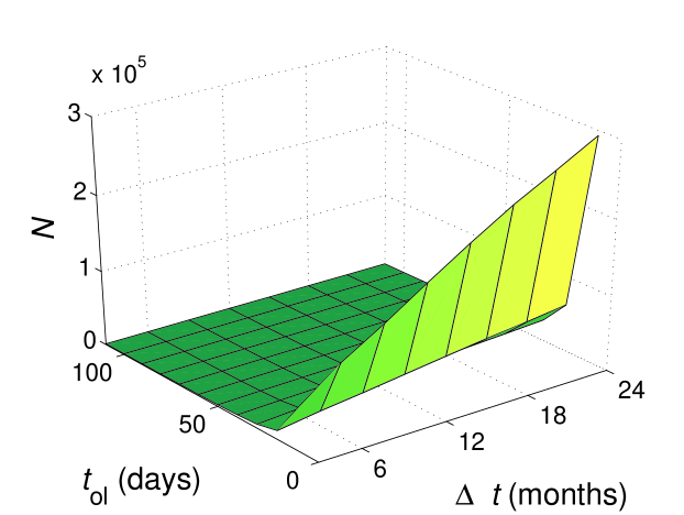
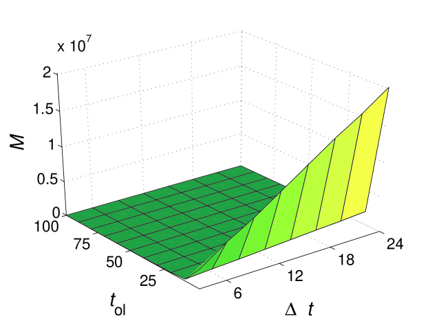
Figure 5: The number of vertices (A) and number of edges (B), $N$ and $M$, as functions of the overlap time $t_{\mathrm{ol}}$ and time window size $\Delta t$.

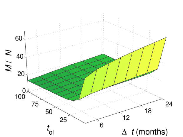
Figure 6: The average number of edges per vertex, $N/M$, as functions of the overlap time $t_{\mathrm{ol}}$ and time window size $\Delta t$.

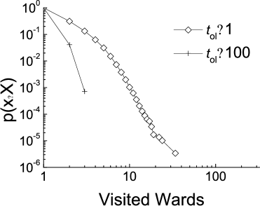
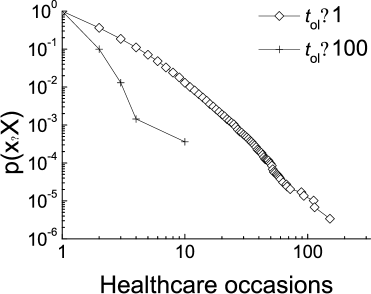
Figure 7: The cumulative distribution, $p(x\geq X)$, for the number of healthcare occasions per inpatient and the number of visited wards per inpatient during the period 2001-2002.

Appendix A Further statistics

The dataset contains information for 570,382 ward admissions, including date of admission, date of discharge, and ward identity. There were a total of 702 wards located at 52 different geographical units such as hospitals and nursing homes. The mean daily number of patients on the wards for the two-year period varied between 1 and 69 (mean 10.05, SD 9.44). Wards with a large number of inpatients per year strongly tend toward shorter duration of inpatient hospital stays, and vice versa, as shown in Figure 4.

As described in the Sect. III, we define a network as the individuals who have been inpatients some time during the sample time, $\Delta t$, and a contact as a link between two individuals who have been inpatients on the same ward for a duration $\geq t_{\mathrm{ol}}$. Figure 5A and 5B show the number of nodes, $N$, and the number of links, $M$, for nodes having at least one link with a duration $\geq t_{\mathrm{ol}}$.

The $N$ and $M$ surfaces show a large variation in absolute size. The surface for the number of vertices per node shows a similar surface. The quote between the largest value and smallest value is, however, smaller by several orders of magnitude.

The number of healthcare occasions and number of different wards visited during the period under study varies a widely for different values of, $t_{\mathrm{ol}}$ (see Figure 7). The number of separate healthcare occasions for all contacts, that is, to $t_{\mathrm{ol}}\geq 1$, in particular exhibits a fat tail. This holds to some extent for the number of visited wards as well. The individuals who had at least one contact with a duration of at least 100 days are thus considerably less mobile between the wards in the hospital system than those who have not.

The dataset is associated with one known systematic bias in the sense that one single inpatient may be registered as an inpatient on two wards at the same time such as when an inpatient is moved for a short period but is expected to return. Our analyses show that one single individual is registered on two separate wards 6734 times. We have not been able to show that these biases have any significant effect on the results we are presenting in this paper and will therefore use the whole dataset in our analyzes.

Figure 8: The best estimates of the slope for different values of for the whole population (A) and for individuals younger than 65 years old (B) The error bars are 95% confidence intervals generated by bootstrapping.

Appendix B Notes on the distribution of hospitalization times

In Figure 8 we have plotted the cumulative distribution, of $t_{\mathrm{dur}}$, for all healthcare occasions in 2001. This allows us to plot the cumulative distribution in the interval 1 to 365 days for all of these healthcare occasions without interference from any finite size effects of the material in this interval. The plot shows that the duration of hospital stays exhibits a skewed power-law-like tail, $p(t_{\mathrm{dur}})\sim t_{\mathrm{dur}}^{-\alpha}$. We estimate the slope, $\alpha$, in the interval $[t_{\mathrm{min}},365]$ by fitting $\alpha$ in $p(t_{\mathrm{dur}})=t_{\mathrm{dur}}^{-\alpha}/\tau$, where

$$\tau=\sum_{i=t_{\mathrm{min}}}^{365}i^{-\alpha}$$ (5)

is a normalization factor. A maximum likelihood procedure was used for the estimation. The 95% confidence intervals were estimated by bootstrapping. Figure 8A and 8B show how $\alpha$ changes when $t_{\mathrm{min}}$ is increased.

Appendix C A model of contact networks of patients

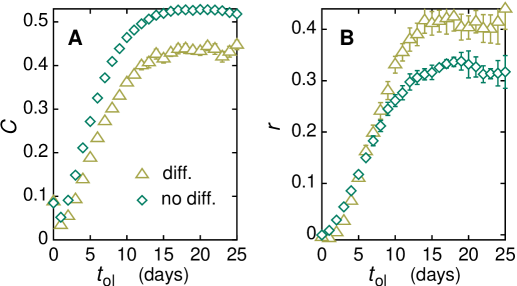
Figure 9: he assortative mixing (A) and clustering coefficients (B) as functions of the overlap time $t_{\mathrm{ol}}$ for a simulated healthcare system. For the “no diff.” curves, patients are assigned to a random ward, whereas for ”diff.” curves, patients with a similar duration of hospital stay share wards (which reproduce the functional forms of Fig. 3). The simulation parameters are $N=10000$, $N_{w}=50$, $p_{1}=0.02$ / day, $p_{2}=1/3$, $\Delta t=2500$ days, and $P_{t}\sim t^{-3}$. The curves are averaged over 10 runs of the algorithm.

To answer the question why $C$ increases with $t_{\mathrm{ol}}$ (for fixed $\Delta t$) we construct a simple agent-based model of a healthcare system from first principles: Suppose a healthcare system of Nw wards of equal capacity is intended to serve a population of $N$ individuals. Each day a non-hospitalized individual hospitalized with a probability $p_{1}$ and will stay for a random time $t$ (of some distribution $P_{t}$) on ward $w$ (how the ward is chosen is discussed below). After hospitalization the patient is either transferred to another ward with probability $p_{2}$ for a duration of a new t or discharged. This dynamic, given a $\Delta t$ and $t_{\mathrm{ol}}$, yields networks just like our real data did.

How shall we assign patients to the wards? The simplest assumption is to choose the wards with equal probability. As seen in Figure 9, this yields the shape of $C$ and $r$ seen in Figure 3.

One important feature is missing from this model: different specialty wards hospitalize patients for different durations. If we incorporate this, the curves stay qualitatively the same. From the model, we understand that for large overlap times the long-term patients form densely connected components—otherwise the network is empty. The model is insensitive to parameter values. A skewed $P_{t}$ function is, however, needed.

The algorithm consists of the following steps repeated t times (that is, one of these steps corresponds to one day in the simulation):

1. Go through all healthy (non-hospitalized) patients. With a probability $p_{1}$ hospitalize a patient. The duration of the hospitalization is given by $P_{t}$. Assign a ward according to the methods listed below. In our simulation, we choose $P_{t}\sim t^{-3}$. This is based on the observed distribution of hospitalization times (see Figure 2).

2. Go through all newly discharged patients. With probability $p_{2}$ re-hospitalize a patient. The duration of the hospitalization is given by $P_{t}$. Assign a ward according to the methods listed below.

3. If needed, construct the network according to the method detailed in the Sect. III.

To assign a ward given a hospitalization time, we propose two different methods. The first option is to select the ward by uniform randomness. Clearly, this will, on average, make all wards equally full. This method is used for the “no diff.” curves in Figure 2. However, the hospitalization times are very different—on some wards, the hospitalization time is much longer than average; on others, people stay for very short periods. To model this, we differentiate strictly between the wards so that the patients on ward $w_{i}$ always stay a shorter time than the patients on ward $w_{i+1}$. We implement this by generating $N_{\mathrm{rnd}}$ random numbers distributed according to $P_{t}$. Then we sort these values in increasing values of $t$ and associate ward 1 with the $t$-values $[t_{1},\ldots,t_{s1}]$, ward 2 with the $t$-values $[t_{s1}+1,\ldots,t_{s2}]$, and so on, such that the sum of $t$-values are the same for all wards. During the iterations, a random value of the array of random numbers is drawn and the patient is assigned to the corresponding pre-assigned ward. We use $N_{\mathrm{rnd}}=10^{6}$ for Figure 9. The same plot with $N_{\mathrm{rnd}}=10^{4}$ yields indistinguishable curves. This is the method used for the “diff.” curves in Figure 9. Finally, to obtain the curves in Figure 9, we average the result of 20 runs of the algorithm above.

References

- (1) Newman, M. E. J. Properties of highly clustered networks. Phys. Rev. E 68, 026121 (2003).
- (2) Newman, M. E. J. Assortative mixing in networks. Phys. Rev. Lett. 89, 208701 (2002).
- (3) Anderson, R. M. & May, R. M. Infectious Diseases of Humans: Dynamics and Control (Oxford University Press, Oxford, 1992).
- (4) Giesecke, J. Modern Infectious Disease Epidemiology (Arnold, London, 2002).
- (5) Watts, D. J. Six Degrees: The Science of a Connected Age (W. W. Norton & Company, New York, 2003).
- (6) Colgate, S. A., Stanley, E. A., Hyman, J. M., Layne, S. P. & Qualls, C. Risk Behavior-Based Model of the Cubic Growth of Acquired Immunodeficiency Syndrome in the United-States. Proc. Natl. Acad. Sci. U.S.A. 86, 4793-4797 (1989).
- (7) Szendroi, B. & Csanyi, G. Polynomial epidemics and clustering in contactnetworks. Proc. R. Soc. Lon. B (Suppl. Biol. Lett.) 271, 356-366 (2004).
- (8) Heymann, D. L. (ed.) Control of Communicable Diseases Manual (American Public Health Association, Washington, 2004).
- (9) Barabási, A. L. & Albert, R. Emergence of scaling in random networks. Science 286, 509-512 (1999).
- (10) Klemm, K. & Eguíluz, V. M. Highly clustered scale-free networks. Phys. Rev. E 65, 036123 (2002).
- (11) Price, D. J. D. General Theory of Bibliometric and Other Cumulative Advantage Processes. J. Am. Soc. Info. Sci. 27, 292-306 (1976).