Noise-enhanced computation in a model of a cortical column
Running title: Noise-aided computation in a cortical model

Abstract

Varied sensory systems use noise in order to enhance detection of weak signals. It has been conjectured in the literature that this effect, known as stochastic resonance, may take place in central cognitive processes such as the memory retrieval of arithmetical multiplication. We show in a simplified model of cortical tissue, that complex arithmetical calculations can be carried out and are enhanced in the presence of a stochastic background. The performance is shown to be positively correlated to the susceptibility of the network, defined as its sensitivity to a variation of the mean of its inputs. For nontrivial arithmetic tasks such as multiplication, stochastic resonance is an emergent property of the microcircuitry of the model network.

Keywords: Stochastic resonance, information processing, recurrent neural network

Contact author: Wulfram.Gerstner@epfl.ch

1 Introduction

Noise is usually considered as having a corrupting effect on meaningful signals. There is however one well known counter example to this widespread belief; the stochastic resonance (SR) phenomenon. In this case, addition of a random interference signal (noise) to a weak, subthreshold stimuli, may enhance its detection. Originally introduced in the framework of physics [1, 2, 3, 4, 5, 6, 7, 8], stochastic resonance is now known to take place in several sensory systems from the cricket cercal sensory system [9], to crayfish mechanoreceptors [10], the somatosensory cortex of the cat [11] and the human visual cortex [12, 13] in order to facilitate detection of weak signals (for a review see [14]).

In addition there is evidence that stochastic resonance may be used not only at the level of sensory processing, but also in central cognitive processes. In a psychophysical study by Usher and Feingold, the memory retrieval of arithmetical multiplication was found to be enhanced by the addition of noise [15].

In this article, we feed a simplified model of a cortical column with two time-varying input signals. We first show that for a broad set of computation based on those input signals, addition of a small amount of noise enhances the computational power of the system. The location where the noise strength is optimal lies approximately where the network reacts the strongest to a change in the mean input (maximum susceptibility). We then set the connectivity to zero (with appropriate scaling of the statistics of the input to the neurons). Although the simplest task (addition of both input signals) can be achieved with a similar accuracy to that obtained with a connected network, a multiplicative task can only be solved if the population of neurons is connected. The stochastic resonance effect is thus seen to take place at the system level [16] rather than at the single cell level. It is an emergent property of the neuronal assemblies.

2 Methods

We consider in our simulations networks of $N=200$ cells (leaky integrate-and-fire neurons). The connectivity matrix is fixed and every neuron receives input from $C_{E}=40$ excitatory and $C_{I}=10$ inhibitory presynaptic neurons randomly chosen among the $N-1$ neurons in the network. The system is made out of $80\%$ excitatory and $20\%$ inhibitory neurons, reflecting the ratio of pyramidal cells to interneurons in cortical tissue. This excess of excitatory neurons is approximately balanced by the greater efficacy of synaptic transmission for inhibition; in our model six times bigger than for excitation: $\omega_{I}=7.2$mV and $\omega_{E}=1.2$mV. This approximate balance between excitation and inhibition is thought to take place at a functional level in cortical areas [17, 18]. Sparsely-connected networks of spiking neurons of this type have been fully described in terms of their dynamical behaviour [19]. The dynamics of the leaky integrate-and-fire neurons is described by the following equation:

$$\tau_{m}\dot{u_{i}}(t)=-u_{i}(t)+RI_{i}^{netw}(t)+RI_{i}^{ext}(t)$$ (1)

where $u_{i}(t)$ describes the membrane potential of neuron $i$ with respect to its equilibrium value $u_{i}=0$, $\tau_{m}=20$ms corresponds to its effective membrane time constant and $R=100M\Omega$ is the effective input resistance of the neuron stimulated by a total input $RI_{i}^{netw}(t)+RI_{i}^{ext}(t)$. We add to this equation a threshold condition; if the membrane potential of the neuron exceeds the critical value $\theta=20$mV, a spike is emitted and after a refractory period $\tau_{rp}=2$ms, the integration start again from the reset potential $u_{reset}=0$mV. Every time the neuron $i$ receives an action potential from a presynaptic pyramidal cell $j$ (resp. interneuron), its membrane potential is depolarized according to the value of the synaptic efficacy for excitation $\omega_{j}=+\omega_{E}$ (resp. for inhibition, the neuron is hyperpolarized by an amount $\omega_{j}=-\omega_{I}$). The input a neuron $i$ will get from within the network can thus be written as:

$$RI_{i}^{netw}(t)=\tau_{m}\sum_{j\in M_{i}}\omega_{j}\sum_{k}\delta(t-t_{j}^{k}-D)$$ (2)

where $M_{i}$ is the ensemble of presynaptic neurons, $t_{j}^{k}$ the time neuron $j$ fires its $k$’th spike and $D=1$ms is a short transmission delay.

We can now decompose the external stimulation $RI_{i}^{ext}(t)$ into two contributions. First, we model all noise sources, ranging from synaptic bombardment from neurons outside the network to different sources of noise diversely located at the level of synaptic transmission, channel gating, ion concentrations, membrane conductance to name but a few. All these noise sources are grouped into a term $RI^{backgr}$ with a mean depolarisation $RI^{dep}$ and a white noise component defined by its standard deviation $RI^{noise}$. We can define the susceptibility $\chi$ of the network as the sensitivity of the population spiking rate $\nu$ upon a change in the mean depolarisation $RI^{dep}$: $\chi=\frac{\partial\nu}{\partial I^{dep}}$. We constrained our simulation space to small mean depolarisation $RI^{dep}$ so that in absence of the noisy component $RI^{noise}(t)$, the network exhibits no spiking activity (subthreshold regime).

Figure 1 :

Then, we inject two test signals $I_{1}(t)$ and $I_{2}(t)$, each to $20\%$ randomly chosen neurons in the network. Both inputs share the same statistical properties; they are constant over a time interval $T=40$ms and then they switch to new randomly chosen values and remain constant for the next time interval $T$. At each transition time, the new values are chosen uniformly over the interval $[-50pA,50pA]$. We want to know how performance in a series of computational tasks based on both test signals $I_{1}(t)$ and $I_{2}(t)$ are affected by the noise level. We adapt a paradigm introduced in the framework of Liquid State Machines [20] or Echo State Networks [21]: we consider a readout with a dynamics $dy/dt=-((y-\alpha_{0})/\tau_{s})+\sum_{i=1}^{N}\alpha_{i}\sum_{k}\delta(t-t_{i}^{k})$ where the sums run over all firing times $t_{i}^{k}$ of all neurons in the network. $\tau_{s}=5$ms is a short synaptic time constant. The $N+1$ free parameters $\alpha_{i}$ ($0\leq i\leq N$) are chosen so as to minimize the signal reconstruction error between the readout and the target: $E=\langle[y(t)-F(I_{1}(t-\Delta),I_{2}(t-\Delta))]^{2}\rangle$. In our simulations we fixed $\Delta=15ms$ so that the transient period after a transition has vanished. The set of functions $F(I_{1},I_{2})$ that are under consideration in the present study are; the addition $F=I_{1}+I_{2}$, the multiplication $F=I_{1}I_{2}$ which plays a crucial role in the transformation of object locations from retinal to body-centered coordinates [23] and two polynomials of degree two $F=(I_{1}+I_{2})^{2}=I_{1}^{2}+I_{2}^{2}+I_{1}I_{2}$ and $F=(I_{1}-I_{2})^{2}=I_{1}^{2}+I_{2}^{2}-I_{1}I_{2}$, which can be seen as the nonlinear XOR paradigm [22].

Parameters were optimized using a first simulation (learning set) lasting 100 seconds (100’000 time steps of simulation) and were kept fixed afterwards. The performance measurements reported in this paper are then evaluated on a second simulation of 100 seconds (test set). We compare our results to a simple two parameter readout. Such a readout only adjusts to the mean of the time series $F(I_{1}(t),I_{2}(t))$. The reconstruction error for such a readout equals the variance $\sigma_{\rm F}^{2}$ of the time series $F(I_{1}(t),I_{2}(t))$. The performance with the full readout are therefore expressed as a gain (in percent) over the trivial prediction: $G=100(1-\frac{E}{\sigma_{\rm F}^{2}})$, where $E$ is the error introduced above.

In the simulation of Fig.3, all connections in the network were removed. In order to compensate the loss of input $I^{netw}$, we changed the background input $RI^{backgr}$ so that the neurons receive an input with the same statistical properties (mean and variance). The adapted input in the network with ”no connection” (nc) is thus: $RI^{dep}_{nc}=RI^{dep}+\nu\tau_{m}(C_{E}\omega_{E}-C_{I}\omega_{I})$ for the mean and $RI^{noise}_{nc}=RI^{noise}+\sqrt{\nu\tau_{m}(C_{E}\omega_{E}^{2}+C_{I}\omega_{I}^{2})}$ for the variance term. $\nu$ is the mean population rate in the connected network (see [19]).

Simulation results were obtained using the simulation software NEST.

3 Results

We want to know how noise influences the ability of a recurrent network of spiking neurons to process information and to perform a series of computational tasks. In particular we are interested in effects related to stochastic resonance. We therefore relate the optimal noise level (where the system has a maximum performance) to dynamical properties of the network. From that perspective, we analyze how performance in a series of computational tasks based on both test signals $I_{1}(t)$ and $I_{2}(t)$ are affected by the noise level. In a first series of simulations, we measure the gain over the trivial prediction for three different functions of the test signals; $F=I_{1}+I_{2}$, $F=(I_{1}+I_{2})^{2}$ and $F=(I_{1}-I_{2})^{2}$ (see figure 2, respectively top right, bottom left and bottom right graphs). Note that the function $F=(I_{1}-I_{2})^{2}$ can be seen as an implementation of the XOR task, which cannot be solved by a single layer neural network (perceptron) [22]. In all three tasks, the network exhibits stochastic resonance; for a given mean depolarisation $RI^{dep}$, there is a non-monotonic dependence upon the noise level. The maximum gain compared to trivial prediction reaches $38\%$ for the additive task and $7-9\%$ for polynomials of degree two. A comparison to the map of the susceptibility of the network $\chi=\frac{\partial\nu}{\partial I^{dep}}$ (see top left graph of figure 2) indicated that the tasks are solved best when the sensitivity of the network upon changes in the mean input is highest. Addition of noise both increases the susceptibility of the network and the capacity of performing complex computation based on sparse inputs.

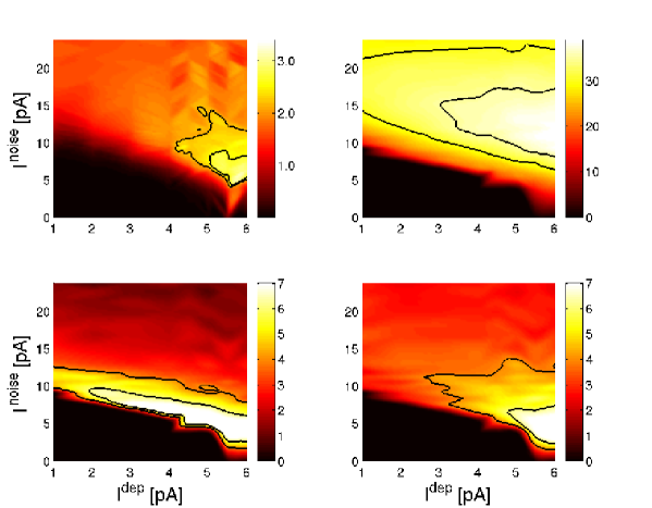
Figure 2 :

In order to know whether stochastic resonance displayed in the network is an emergent property of the population of neuron [16] or a single cell effect, we removed all connections within the network. In this second series of simulations, we compare the performance achieved in networks with connectivity to networks with no connectivity. The latter networks receive adapted version of the mean input $RI^{dep}_{nc}$ and of the noisy input $RI^{noise}_{nc}$ so that every neurons is stimulated with a mean and variance equivalent to that of the connected network (see methods).

In the first task; the addition $F=I_{1}+I_{2}$, the performance with and without connectivity are similar (see figure 3 left). Since the readout unit performs a weighted sum that runs over all neurons, it can capture the essence of this simple computation by summing the averaged response of the groups of neurons receiving input $I_{1}$ with the averaged response of those receiving $I_{2}$. Recurrent loops play here no significative role. In the second task we train the network to perform the multiplication of the two test signals $F=I_{1}I_{2}$. This arithmetical operation is thought to be essential to the brain in order to do coordinate transformation [23]. The computation of a multiplication by a recurrent neural network was shown to be achievable in a model of the parietal cortex [24, 25]. In this multiplicative task $F=I_{1}I_{2}$, the complex recurrent network outperforms the network with no connectivity (see figure 3 right). In fact, in absence of connections within the population of neurons, multiplication cannot be solved by the simple addition of noise. Stochastic resonance displayed in the multiplicative task therefore takes place at a system level rather than at the level of single neurons.

Figure 3 :

4 Conclusion

Complex networks of neurons fall in the class of non linear systems with a threshold; systems that are known to exhibit stochastic resonance. From the experimental side, evidences have shown that the phenomenon helps in detecting sensory signals of small amplitude, and furthermore to favor high level cognitive processes such as arithmetical calculations. Our model has revealed the presence of stochastic resonance in a series of neural-based computation. Whereas simple additive transformations of input signals can be solved by a collection of independent neurons, more complex computations need the massive recurrence typically observed in cortical tissue. Such complex tasks include the XOR problem, a nonlinear benchmark test, and the arithmetical multiplication the brain is likely to use in order to achieve coordinate transformation. Stochastic resonance displayed is then an emergent property of the brain microcircuitry.

References

- [1] R. Benzi, A. Sutera, and A. Vulpiani. The mechanism of stochastic resonance. J. Phys. A, 14:453–457, 1981.
- [2] K. Wiesenfeld and F. Jaramillo. Minireview of stochastic resonance. Chaos, 8:539–548, 1998.
- [3] J. J. Collins, Carson C. Chow, Ann C. Capela, and Thomas T. Imhoff. Aperiodic stochastic resonance. Physical Review E, 54:5575–5584, 1996.
- [4] L. Gammaitoni, F. Marchesoni, and S. Santucci. Stochastic resonance as a bona fide resonance. Phys. Rev. Lett., 74:1052–1055, 1995.
- [5] L. Gammaitoni, P. Hänggi, P. Jung, and F. Marchesoni. Stochastic resonance. Rev Mod Phys, 70:223–287, 1998.
- [6] B. McNamara and K. Wiesenfeld. Theory of stochastic resonance. Physical Review A, 39:4854–4869, 1989.
- [7] K. Wiesenfeld, D. Pierson, E. Pantazelou, and F. Moss. Stochastic resonance on a circle. Phys. Rev. Lett., 72:2125–2129, 1994.
- [8] K. Wiesenfeld and F. Moss. Stochastic resonance and the benefits of noise: from ice ages to crayfish and squids. Nature, 373:33–36, 1995.
- [9] J.E. Levin and J.P. Miller. Broadband neural encoding in the cricket cercal sensory system enhanced by stochastic resonance. Nature, 380:165–168, 1996.
- [10] J.K. Douglass, L. Wilkens, E. Pantazelou, and F. Moss. Noise enhancement of information transfer in crayfish mechanoreceptors by stochastic resonance. Nature, 365:337–340, 1993.
- [11] T. Mori and S. Kai. Noise-induced entrainment and stochastic resonance in human brain waves. Phys. Rev. Lett., 88(218101), 2002.
- [12] K. Kitajo, D. Nozaki, L.M. Ward, and Y. Yamamoto. Behavioral stochastic resonance within the human brain. Phys. Rev. Lett., 90(218103), 2003.
- [13] I. Hidaka, D. Nozaki, and Y. Yamamoto. Functional stochastic resonance in the human brain: Noise induced sensitization of baroreflex system. Phys. Rev. Lett., 85(17), 2000.
- [14] F. Moss, L. M. Ward, and W. G. Sannita. Stochastic resonance and sensory information processing: a tutorial and review of application. Clinical Neurophysiology, 115:267–281, 2004.
- [15] M. Usher and M. Feingold. Stochastic resonance in the speed of memory retrieval. Biological Cybernetics, 83:11–16, 2000.
- [16] N. Masuda and K. Aihara. Bridging rate coding and temporal spike coding by effect of noise. Physical Review Letters, 88(248101), 2002.
- [17] G. S. Liu. Local structural balance and functional interaction of excitatory and inhibitory synapses in hippocampal dendrites. Nat. Neurosci., 7(4):373–379, 2004.
- [18] Y. Shu and A. A. McCormick A. Hasentraub. Turning on and off recurrent balanced cortical activity. Nature, 423:288–293, 2003.
- [19] N. Brunel. Dynamics of sparsely-connected networks of excitatory and inhibitory neurons. J. of Computational Neuroscience, 8:183–208, 2000.
- [20] W. Maass, T. Natschläger, and H. Markram. Real-time computing without stable states: A new framework for neural computation based on perturbations. Neural Computation, 14(11):2531–2560, 2002.
- [21] H. Jaeger and H. Haas. Harnessing nonlinearity: Predicting chaotic systems and saving energy in wireless communication. Science, 304:78–80, 2004.
- [22] M. L. Minsky and S. A. Papert. Perceptrons. MIT Press, Cambridge Mass., 1969.
- [23] R. A. Andersen, R. M. Bracewell, S. Barash, J. W. Gnadt, and L. Fogassi. Eye position effects on visual, memory, and saccade-related activity in areas lip and 7a of macaque. J. Neurosci., 10:1176–1198, 1990.
- [24] E. Salinas and L.F. Abbott. A model of multiplicative neural responses in parietal cortex. Proc. Natl. Academy Sci. USA, 93:11956–11961, 1996.
- [25] A. Pouget and T. J. Sejnowski. Spatial transformations in the parietal cortex using basis functions. Journal of Cognitive Neuroscience, 9(2):222–237, 1997.