Strong-coupling dynamics of a multi-cellular chemotactic system

Abstract

Chemical signaling is one of the ubiquitous mechanisms by which inter-cellular communication takes place at the microscopic level, particularly via chemotaxis. Such multi-cellular systems are popularly studied using continuum, mean-field equations. In this letter we study a stochastic model of chemotactic signaling. The Langevin formalism of the model makes it amenable to calculation via non-perturbative analysis, which enables a quantification of the effect of fluctuations on both the weak and strongly-coupled biological dynamics. In particular we show that the (i) self-localization due to auto-chemotaxis is impossible. (ii) when aggregation occurs, the aggregate performs a random walk with a renormalized diffusion coefficient $D_{R}\propto\epsilon^{-2}N^{-3}$. (iii) the stochastic model exhibits sharp transitions in cell motile behavior for negative chemotaxis, behavior which has no parallel in the mean-field Keller-Segel equations.

The study of biological systems through modeling is a promising endeavor to understand or throw light on the macroscopic complexity originating from the microscopic cellular interactions common to all living organisms. At the microscopic level, cells interact with each other through various means, principally via local short-range forces such as adhesion and through long-range forces mediated via chemical signals. In many cases, cells do not just respond to chemical signals but are actively involved in their production also. This signal feedback leads to intricate inter-cellular communication, which is the main mechanism behind the emergence of the observed complex behavior of multi-cellular systems. An important aspect of the feedback mechanism is that the cells’ dynamics are typically dominated by long range spatio-temporal correlations. Modeling has traditionally been approached through the construction of coupled partial differential equations, describing the evolution of a density field $\rho$, representing the number density of cells. Many of these models are variants of the Keller-Segel equations Keller (1). Recently it has been shown that the derivation of the latter equations from a microscopic, stochastic Langevin model of interacting cells, is achieved by neglecting cell-cell correlations Newman (2); indeed this verifies the hypothesis that Keller-Segel variants are mean-field type models i.e. they are applicable to modeling biological situations in which the cell number density is sufficiently large. This statement is however qualitative; it is not clear what are the similarities and differences predicted by the stochastic models and their deterministic counterparts.

In this letter we study a stochastic model of chemotactic signaling; this being an individual-based model of cells interacting via long-range chemical signals and actively responding to such signals via chemotaxis. Such models have been previously studied by a number of authors (see for example Othmer (3), Stevens (4), Jiang (5), Hadeler (6), Merks (7) ). We shall show that it is possible to gain an understanding of the cells’ strongly-correlated dynamics by means of a non-perturbative analysis applied directly on the Langevin equation formalism of the model. This will give us an analytical quantitative way of comparing the stochastic and deterministic models. It is to be emphasized that the non-perturbative nature of the analysis method will enable us to obtain insight, otherwise not obtainable via the conventional perturbative approach Newman (2) or through analysis of the corresponding mean-field type equations. The system we shall analyze consists of $N$ chemotactic cells which are constantly secreting a chemical (whose concentration is denoted by $\phi$) and which respond to the local chemical gradient by either moving up the gradient (positive chemotaxis) or down the gradient (negative chemotaxis). The latter leads to dispersion whereas the former effect leads to aggregation. Such mechanisms are common to many organisms including amoeba, myxobacteria, leucocytes, and germ cells. We shall first treat the case of a single self-interacting cell, then extend it to the multi-cellular case. The equations defining the single-cell stochastic model are Newman (2):

$${\dot{\bf x}_{c}}(t) ={\bf\xi}(t)+\kappa\alpha\nabla\phi({\bf x}_{c},t),$$ (1)

$$\partial_{t}\phi({\bf x},t) =D_{1}\nabla^{2}\phi({\bf x},t)-\lambda\phi({\bf x},t)+\beta\delta({\bf x}-{\bf x}_{c}(t)).$$ (2)

Eq.1 is a Langevin equation describing the motion of a cell whose position at time $t$ is denoted as ${\bf x}_{c}(t)$. The stochastic variable $\xi$ is white noise defined through $\langle\xi^{a}(t)\rangle=0$ and $\langle\xi^{a}(t)\xi^{b}(t^{\prime})\rangle=2D_{0}\delta_{a,b}\delta(t-t^{\prime})$ where $a$ and $b$ refer to the spatial components of the noise vectors. In the absence of a chemical gradient, the cell performs a pure random walk characterized by a diffusion coefficient $D_{0}$. In the presence of a chemical gradient, the cell has a velocity $\kappa\alpha\nabla\phi$ superimposed on the random walk, where $\alpha$ is a positive constant typifying the strength of chemotaxis and $\kappa$ is a constant which can take the values $-1$ (negative chemotaxis) or $1$ (positive chemotaxis). The overall effect is a random walk biased in the direction of increasing chemical concentration ($\kappa=1$) or in the direction of decreasing chemical concentration ($\kappa=-1$). Eq.2 is a reaction-diffusion equation describing the chemical dynamics. The chemical diffuses with diffusion coefficient $D_{1}$, decays in solution at a rate $\lambda$ and is secreted by the cell at a rate $\beta$. The feedback mechanism is what makes this problem non-trivial. The cell constantly modifies its environment through its continuous chemical secretion and simultaneously reacts to its environment via chemotactic sensing and directed motion. For positive chemotaxis, the net effect of the two coupled equations gives rise to a random walk having a larger probability of visiting spatial areas which it has previously visited than of visiting previously unexplored regions. For negative chemotaxis, the opposite situation occurs: the walker is “repelled” away from regions which it has previously visited. The self-interaction of a cell will be referred to as auto-chemotaxis.

The strong non-Markovian nature of the dynamics is what makes this and similar problems (involving self-interacting random walks) difficult to analyze. In this letter we introduce a non-perturbative method to explore the strong-coupling aspects of the theory. Unlike perturbation theory in the coupling parameter $\epsilon=\alpha\beta$ Newman (2), this method can be applied directly to the Langevin formulation of the model i.e. the analysis bypasses the conventional derivation of the equations of motion for the single and multi-cell probability distributions. Integrating the chemical equation Eq.2, assuming that there is no chemical initially $\phi(\mathbf{x},0)=0$, one finds an expression for the local chemical gradient sensed by the cell at time $t$:

$$\nabla\phi=-\frac{\beta}{2}(4\pi t)^{-d/2}D_{1}^{-(1+d/2)}\int\limits_{\tau/t}^{1}du\frac{[\mathbf{x}_{c}(t)-\mathbf{x}_{c}(t-ut)]}{u^{1+d/2}}\\ \times\exp\Biggl{[}-\lambda tu-\frac{[x_{c}(t)-x_{c}(t-ut)]^{2}}{4D_{1}tu}\Biggr{]},$$ (3)

where $d$ is the dimensionality of space and $\tau$ is a refractory period i.e a period of time in which the cell is not sensitive to chemical signals, introducing an effective time delay between signal emission and signal transduction. Another way of stating this is that the cell at time $t$ senses the local gradient due to chemical production in the period $t^{\prime}\in(0,t-\tau)$. Such an effect is a common feature of many chemotactic cells Bray (8). The introduction of $\tau$ also regularizes the integral in Eq.3. Although it is in general impossible to solve this integral, since this requires full knowledge of all previous cell positions, in the asymptotic limit $t\gg 1/\lambda$ the integral is dominated by small $u$ Murray (9). It may therefore be simplified by use of the approximation $\mathbf{x}_{c}(t)-\mathbf{x}_{c}(t-ut)\simeq ut{\dot{\bf x}_{c}}(t)$. We further introduce two convenient variables: $\gamma=2\epsilon\pi^{-d/2}(4D_{1})^{-(1+d/2)}$ and $\lambda^{\prime}=\lambda+\frac{[{\dot{x}_{c}}(t)]^{2}}{4D_{1}}$. Substituting the resulting expression for the chemical gradient in the Langevin equation for the cell we get

$${\dot{\bf x}_{c}}(t)={\bf\xi}(t)-\kappa{\dot{\bf x}_{c}}(t)\Biggl{[}t^{1-d/2}\gamma\int\limits_{\tau/t}^{1}du\frac{e^{{-\lambda^{\prime}tu}}}{u^{d/2}}\Biggr{]}.$$ (4)

Thus we have showed that the long time dynamics of a self-interacting chemotactic cell can be described by a modified Langevin type equation. The explicit computation of the integral on the R.H.S of Eq.(4) leads to the following expressions for $d=1,2$ and 3 respectively

$${\dot{\bf x}_{c}} ={\bf\xi}-\kappa\frac{\epsilon(1-erf\sqrt{\lambda\tau})\dot{\bf x}_{c}}{4D_{1}^{3/2}\sqrt{\lambda}}\biggl{(}{1+\frac{{\dot{x}_{c}}^{2}}{4D_{1}\lambda}}\biggr{)}^{-1/2},$$ (5)

$${\dot{\bf x}_{c}} ={\bf\xi}-\kappa\frac{\epsilon}{8\pi D_{1}^{2}}Ei\Biggl{(}\lambda\tau+\frac{\tau{\dot{x}_{c}}^{2}}{4D_{1}}\Biggr{)}{\dot{\bf x}_{c}},$$ (6)

$${\dot{\bf x}_{c}} ={\bf\xi}-\kappa\frac{\epsilon}{8\pi^{3/2}D_{1}^{5/2}\sqrt{\tau}}\Biggl{(}1-\sqrt{\pi\lambda\tau+\pi\frac{\tau{\dot{x}_{c}}^{2}}{4D_{1}}}\Biggr{)}{\dot{\bf x}_{c}}.$$ (7)

Note that the the function $Ei(x)$ in Eq.(6) refers to the exponential integral. In many biological cases it is found that $\zeta=D_{0}/D_{1}\ll 1$ (for example $\zeta=1/40-1/400$ for Dictyostelium Hofer (10) and $\zeta\simeq 1/30$ for microglia cells and for neutrophils Keshet (11)) and so the above triad of equations simplify by noticing that to a first approximation we have $\langle{\dot{x}_{c}}^{2}\rangle\ll 4D_{1}\lambda$. Note that this entails replacing the magnitude of the velocity squared ${\dot{x}_{c}}^{2}$ in Eqs.(5–7) by its average over noise $\langle{\dot{x}_{c}}^{2}\rangle$. Then the equations are all reduced to the Langevin form for a pure random walk, with a dimensionally-dependent renormalized cell diffusion coefficient $D_{r}$ of the form:

$$D_{r}={D_{0}}(1+\kappa\tilde{\epsilon}_{d})^{-2},$$ (8)

where

$$\tilde{\epsilon}_{1} =\frac{\epsilon(1-erf\sqrt{\lambda\tau})}{4D_{1}^{3/2}\sqrt{\lambda}},$$ (9)

$$\tilde{\epsilon}_{2} =\frac{\epsilon Ei(\lambda\tau)}{8\pi D_{1}^{2}},$$ (10)

$$\tilde{\epsilon}_{3} =\frac{\epsilon}{8\pi^{3/2}D_{1}^{5/2}\sqrt{\tau}}.$$ (11)

The expressions for $D_{r}$ are consistent provided they do not invalidate the initial assumption $\langle{\dot{x}_{c}}^{2}\rangle\ll 4D_{1}\lambda$. It is easy to show that the above treatment is justified given that the inequality $D_{r}/2D_{1}\lambda\delta t\ll 1$ is met, where $\delta t$ is a typical correlation time for the cell’s direction of movement. The inequality verifies our initial approximation used in deriving Eq.(8), namely that the condition $\zeta\ll 1$ allows us to neglect the factor ${\dot{x}_{c}}^{2}/4D_{1}\lambda$ in Eqs.(5–7). The validity of our results is also confirmed by numerical simulations. Fig.1 shows a plot of $D_{r}/D_{0}$ versus the coupling strength $\epsilon$ for three different ratios of $\zeta$ in one dimension ($\kappa=1$).

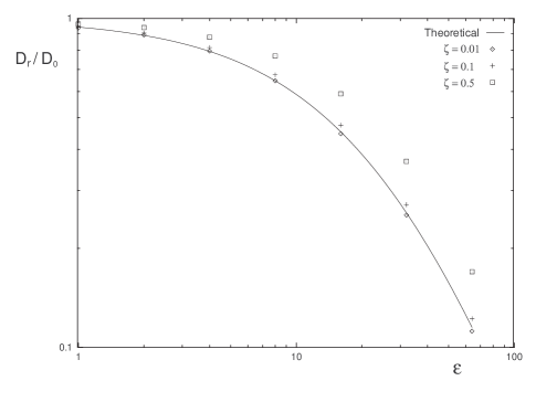
Figure 1: Renormalization of the single cell diffusion coefficient in one dimension. The parameters used are $D_{1}=10$, $\lambda=0.05$, and $\delta t=0.3$. The number of samples taken is 5 $\times$ $10^{4}$. $D_{0}$ is 0.1 for the circle data points, 1.0 for the plus data points, and 5.0 for the square data points. The solid line is the prediction from the non-perturbative method in the limit of small $\zeta$.

Expanding the equations for $D_{r}$ in a power series for $\epsilon$ up to and including terms in $\epsilon^{2}$, we find that these expressions agree exactly with those from first and second-order perturbation theory in the limit of small $\zeta$ Newman (2). The advantage of the non-perturbative method over its perturbative cousin, is its simplicity and its theoretical validity for all coupling strengths. The non-perturbative results suggestively indicate that for positive chemotaxis ($\kappa=1$), for large coupling $\epsilon$ independent of the values of $D_{0}$, $D_{1}$ and $\lambda$ (provided $\lambda>0$) the cell’s asymptotic motion can be described by a random walk with a renormalized diffusion coefficient. In particular we have the prediction $D_{r}\propto\epsilon^{-2}$. Since $D_{r}$ is always positive and greater than zero this clearly shows that self-localization due to auto-chemotaxis is impossible in all dimensions. Applying the same methodology to solving the case of $N$ interacting cells, one finds that contrary to the single cell case it is not possible to decouple the equations in such a way so as to determine an approximate equation of motion for each cell. However it is possible to determine an equation of motion for the center of mass of the interacting cells. In particular one finds that if aggregation occurs then the center of mass of the aggregate has a renormalized diffusion coefficient

$$D_{R}=D_{0}N^{-1}\biggl{[}1+N\gamma\int\limits_{\tau/t}^{1}du\frac{e^{{-\lambda tu}}}{u^{d/2}}\biggr{]}^{-2}.$$ (12)

In the limit of large coupling strength, independent of dimension $d$, the above equation is reduced to the simple form $D_{R}\propto\epsilon^{-2}N^{-3}$. The latter implies that fluctuations in the position of the center of mass decrease as $N^{-3/2}$ (Note that in the absence of chemotaxis i.e. $\epsilon=0$, the fluctuations decrease as $N^{-1/2}$, as expected). In the mean-field equations, the center of mass corresponds to the quantity $\int d^{d}x\ {\bf{x}}\ \rho({\bf{x}},t)/\int d^{d}x\ \rho({\bf{x}},t)$. For the case of aggregation, the latter quantity agrees with the mean position of the center of mass obtained from the stochastic model. However note that whereas the mean-field equations can only give information about the average position of the center of mass of the aggregate, the stochastic equations characterize the fluctuations about this mean. These fluctuations may play an important role in the fusion of two separate but close aggregates in which the number of cells is not very large. Such a phenomenon would lead to different temporal evolution histories (though not necessarily a different final outcome) between the stochastic and mean-field equations.

We now turn our attention to the case of a cell self-interacting via negative chemotaxis i.e $\kappa=-1$. Renormalized diffusion, Eq.(8), is the cell’s asymptotic behavior; this is exactly as for positive chemotaxis, though now $D_{r}>D_{0}$. However note that $D_{r}$ has a singularity when the coupling strength equals a certain critical value given by $\tilde{\epsilon}_{d}=1$. This indicates a possible transition from renormalized diffusive motion (for weak coupling) to a different type of motile behavior. Since we are postulating a transition to behavior other than diffusion, the relevant parameter to investigate is $\Lambda$ which is defined through the mean square displacement of the cell as: $\langle x_{c}^{2}\rangle\propto t^{\Lambda}$. Numerical simulations in one dimension show that asymptotically $\Lambda=1$ for $\epsilon<4D_{1}^{3/2}\sqrt{\lambda}$ whereas for $\epsilon>4D_{1}^{3/2}\sqrt{\lambda}$ invariably we have $\Lambda=2$ (Fig. 2). We shall refer to this phase as ballistic. For $\epsilon$ very close to the critical point we find that the system takes a very long time to stabilize into its asymptotic limit, a feature typical of phase transitions in physical systems Kadanoff (12).

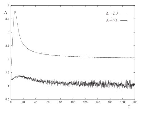
Figure 2: Graph showing the asymptotic value of $\Lambda$ for two values of the parameter $\Delta=\epsilon/4D_{1}^{3/2}\sqrt{\lambda}$ in one dimension. For $\Delta<1$, the asymptotic value of $\Lambda$ is unity, while for $\Delta>1$, $\Lambda$ takes the value of 2. This result supports the transition predicted by theory. $\Lambda$ is computed using the relation $\Lambda=d(\log\langle x_{c}^{2}\rangle)/d(\log t)$. For the case $\Delta=2$, data is averaged over $10^{4}$ samples whereas 2 $\times$ $10^{5}$ samples were used for $\Delta=0.5$. The parameter values used are $D_{0}=0.01$, $D_{1}=1$, $\lambda=0.1$ and $\delta t=0.1$. Note that $\tau$ is chosen small enough so that it satisfies the condition $erf\sqrt{\lambda\tau}<<1$.

It is possible to gain some understanding on the nature of the transition by temporarily ignoring the noise vector $\xi$ in equations Eqs.(5–7), and analyzing the then deterministic equations. Note that ignoring the noise is plausible for the case $\zeta\ll 1$ since this qualitatively implies that the noise term is small compared to the velocity term in the Langevin equation Eq.1. For positive chemotaxis ($\kappa=1$), the only solution in all dimensions is the trivial solution ${\dot{\bf x}_{c}}=0$. Thus if the cell is momentarily perturbed from its original position, it will move for a short time and then come to a complete halt, signifying the stability of the equilibrium state. This stability is independent of the strength of the perturbation or the time at which the perturbation is applied as long as the perturbation is not continuous. This result is also compatible with the form of the renormalized diffusion coefficients derived for positive chemotaxis i.e. in the limit of very strong coupling (chemotaxis dominating over the noise) the cell motility becomes very small. For negative chemotaxis ($\kappa=-1$), there exist two real solutions: the trivial solution ${\dot{\bf x}_{c}}=0$ and a non-zero solution obtained through algebraically solving for the cell velocity. For $\tilde{\epsilon}_{d}<1$, the only solution is the trivial solution however for $\tilde{\epsilon}_{d}>1$, both solutions are possible. This means that for weak coupling, a cell which is perturbed from its original position, wanders around and eventually stops moving. However for coupling strengths larger than a critical coupling strength if the cell is perturbed from its original state then it will move with constant speed in the same direction in which it was originally perturbed. In this case the equilibrium state is unstable. Thus the zero noise analysis predicts the observed sharp transition in $\Lambda$ at the critical coupling $\tilde{\epsilon}_{d}=1$, for small $\zeta$. The expressions for the deterministic cell velocity ($\tilde{\epsilon}_{d}>1$) obtained from such a treatment are also found to be in good agreement with the the root mean square cell position divided by the time, obtained from simulations. It is interesting to note that in-vitro experiments investigating the negative chemotaxis phase of an initially compact aggregate of Dictyostelium, show that the cells’ displacement is proportional to time and not to the square root of time as normal non-chemotactic cells do Keating (13). This is concordant with our theory, since for an initially dense aggregate of cells, dispersion forces the self-interaction of cells to take over the asymptotic dynamics i.e. ballistic behavior is the predicted outcome. It is notable that such behavior is not obtained from the Keller-Segel equations (the equations referred to in this case are the Keller-Segel equations Keller (1) with a negative $\alpha$ instead of a positive one, as is usually the case for positive chemotaxis).

Concluding we have shown that (i) a single cell self-interacting via positive chemotaxis ($D_{0}\ll D_{1}$) performs a random walk characterized by a renormalized diffusion coefficient $D_{r}>0$. This implies that the self-localization of a single chemotactic cell is impossible, independent of the strength of the coupling between the cell and the chemical field. (ii) a system of cells aggregating via positive chemotaxis leads to an aggregate whose center of mass performs a random walk with a renormalized diffusion coefficient. The latter characterizes the fluctuations about the center of mass, information not given by the mean-field model. For large coupling, fluctuations in the aggregate center of mass decrease as $N^{-3/2}$ and thus in this regime, the differences in the temporal evolution predicted by the stochastic and mean-field equations may not be very large. This may explain why the mean-field models have been successful at qualitatively modeling a number of chemotactic phenomena. For biological cases where $\gamma$ is not large, the fluctuations are considerably larger and thus the differences between the two types of models may be more pronounced. (iii) Negative chemotaxis results in either diffusive or ballistic behavior. Whereas for chemotactic aggregation, one could argue that the mean-field model equations (i.e. the Keller-Segel equations) become a better description at later times, when the cell number density becomes large, this is not the case for dispersion via negative chemotaxis. This is borne out by our simulations. Indeed this may apply to any system which involves cellular interactions via negative chemotaxis (e.g. the directional control of axonal growth in the wiring of the nervous system during embryogenesis Painter (14)).

It is a pleasure to thank Timothy Newman for interesting discussions. The author gratefully acknowledges partial support from the NSF (DEB-0328267, IOB-0540680).

References

- (1) E.F. Keller and L.A. Segel, J.Theor.Biol 26, 399 (1970)
- (2) T. J. Newman and R. Grima, Phys. Rev. E. 70, 051916 (2004)
- (3) H. Othmer and A. Stevens, SIAM J. Appl. Math 57, 1044 (1997)
- (4) A. Stevens, SIAM J. Appl. Math 61, 183 (2000)
- (5) Y. Jiang, H. Levine and J.A. Glazier, Biophys. J. 75, 2615 (1998)
- (6) K.P. Hadeler, T. Hillen and F. Lutscher, Math. Mod. Meth. Appl. Sci. 14, 1561 (2004)
- (7) R.M.H. Merks and J.A. Glazier, Physica A 352, 113 (2005)
- (8) D. Bray, Cell Movements (Garland Publishing, New York and London, 1992)
- (9) J. D. Murray, Asyptotic Analysis (Clarendon Press, Oxford, 1974)
- (10) T. Hofer, J. A. Sherratt, and P. K . Maini, Physica D 85, 425 (1995)
- (11) M. Luca, A. Chavez-Ross, L. Edelstein-Keshet, and A. Mogilner, Bull. Math. Biol. 65, 693 (2003)
- (12) L. Kadanoff, Statistical Physics: Statics, Dynamics, and Renormalization (World Scientific, New Jersey, 2000)
- (13) M.T. Keating and J.T. Bonner, J. Bacteriol. 130, 144 (1977)
- (14) K.Painter, P.Maini, and H.Othmer, J.Math. Biol 41, 285 (2000)