Estimation of protein folding probability from equilibrium simulations

Abstract

The assumption that similar structures have similar folding probabilities ($p_{fold}$) leads naturally to a procedure to evaluate $p_{fold}$ for every snapshot saved along an equilibrium folding-unfolding trajectory of a structured peptide or protein. The procedure utilizes a structurally homogeneous clustering and does not require any additional simulation. It can be used to detect multiple folding pathways as shown for a three-stranded antiparallel $\beta$-sheet peptide investigated by implicit solvent molecular dynamics simulations.

I introduction

The folding probability ($p_{fold}$) of a protein conformation saved along a Monte Carlo or molecular dynamics (MD) trajectory is the probability to fold before unfolding Du et al. (1998). It is a useful measure of kinetic distance from the folded, i.e., functional state, and can be used to validate transition state ensemble (TSE) structures, which should have $p_{fold}\approx 0.5$. Such validation consists of starting a large number of trajectories from putative TSE structures with varying initial distribution of velocities and counting the number of those that fold within a ”commitment” time which has to be chosen much longer than the shortest time-scales of conformational fluctuations and much shorter than the average folding time Hubner et al. (2004). The concept of $p_{fold}$ calculation originates from a method for determining transmission coefficients, starting from a known transition state Chandler (1978) and the identification of simpler transition states in protein dynamics (e.g., tyrosine ring flips) Northrup et al. (1982). The approach has been used to identify the otherwise very elusive folding TSE by atomistic Monte Carlo off-lattice simulations of small proteins with a $G\bar{o}$ potential Li and Shakhnovich (2001); Hubner et al. (2004), as well as implicit solvent MD Gsponer and Caflisch (2002); Rao and Caflisch (2004) and Monte Carlo Lenz et al. (2004) simulations with a physico-chemical based potential. The number of trial simulations needed for the reliable evaluation of $p_{fold}$ makes the estimation of the folding probability computationally very expensive. For this reason, here we propose a method to estimate folding probabilities for all structures visited in an equilibrium folding-unfolding trajectory without any additional simulation.

II Methods

Table 1: DRMS clusters used for the calculation of $P_{f}$.

Cluster	$P_{f}^{C}$	$P_{f}$	$\sigma_{p_{fold}}$	$N$	$W$	$W_{sample}$
1	0.00	0.03	0.04	150	144	15
2	0.11	0.05	0.06	150	449	15
3	0.06	0.05	0.07	120	36	12
4	0.08	0.07	0.08	140	555	14
5	0.10	0.08	0.06	100	10	10
6	0.13	0.12	0.18	160	911	16
7	0.25	0.16	0.07	80	4	4
8	0.23	0.20	0.31	150	141	15
9	0.21	0.22	0.15	140	178	14
10	0.12	0.23	0.20	120	48	12
11	0.57	0.25	0.14	140	14	14
12	0.05	0.27	0.19	100	19	10
13	0.23	0.29	0.38	140	391	14
14	0.08	0.30	0.15	120	12	12
15	0.72	0.35	0.23	130	129	13
16	0.19	0.38	0.18	130	26	13
17	0.38	0.44	0.39	160	16	16
18	0.38	0.51	0.28	160	16	16
19	0.65	0.60	0.29	100	20	10
20	0.57	0.61	0.35	70	7	7
21	0.48	0.63	0.32	140	27	14
22	0.74	0.65	0.40	140	539	14
23	0.68	0.66	0.18	140	28	14
24	0.38	0.71	0.24	130	13	13
25	0.50	0.72	0.20	100	2	2
26	0.82	0.76	0.31	170	17	17
27	0.50	0.78	0.14	120	12	12
28	0.78	0.78	0.22	180	18	18
29	0.70	0.79	0.19	130	189	13
30	0.77	0.79	0.17	150	30	15
31	0.85	0.81	0.11	130	13	13
32	0.91	0.83	0.20	140	401	14
33	0.90	0.85	0.27	100	20	10
34	0.85	0.85	0.10	120	48	12
35	0.94	0.88	0.13	170	1990	17
36	0.71	0.94	0.07	70	7	7
37	0.95	0.95	0.06	150	855	15

II.1 Molecular dynamics simulations

Beta3s is a designed 20-residue sequence whose solution conformation has been investigated by NMR spectroscopy De Alba et al. (1999). The NMR data indicate that beta3s in aqueous solution forms a monomeric (up to more than 1mM concentration) triple-stranded antiparallel $\beta$-sheet, in equilibrium with the denatured state De Alba et al. (1999). We have previously shown that in implicit solvent Ferrara et al. (2002) molecular dynamics simulations beta3s folds reversibly to the NMR solution conformation, irrespective of the starting structure Ferrara and Caflisch (2000). Recently, four molecular dynamics simulations of beta3s were performed at 330 K for a total simulation time of 12.6 $\mu$s Cavalli et al. (2003). There are 72 folding events and 73 unfolding events and the average time required to go from the denatured state to the folded conformation is 83 ns. The 12.6 $\mu$s of simulation length is about two orders of magnitude longer than the average folding or unfolding time, which are similar because at 330 K the native and denatured states are almost equally populated Cavalli et al. (2003). For the $p_{fold}$ analysis the first 0.65 $\mu$s of each of the four simulations were neglected so that along the 10 $\mu$s of simulations there are a total of 500000 snapshots because coordinates were saved every 20 ps.

The simulations were performed with the program CHARMM Brooks et al. (1983). Beta3s was modeled by explicitly considering all heavy atoms and the hydrogen atoms bound to nitrogen or oxygen atoms (PARAM19 force field Brooks et al. (1983)). A mean field approximation based on the solvent accessible surface was used to describe the main effects of the aqueous solvent on the solute Ferrara et al. (2002). The two surface tension-like parameters of the solvation model were optimized without using beta3s. The same force field and implicit solvent model have been used recently in molecular dynamics simulations of the early steps of ordered aggregation Gsponer et al. (2003), and folding of structured peptidesFerrara et al. (2002); Ferrara and Caflisch (2000), as well as small proteins of about 60 residues Gsponer and Caflisch (2001). Despite the absence of collisions with water molecules, in the simulations with implicit solvent the separation of time scales is comparable with that observed experimentally. Helices fold in about 1 ns Ferrara et al. (2000), $\beta$-hairpins in about 10 ns Ferrara et al. (2000) and triple-stranded $\beta$-sheets in about 100 ns Cavalli et al. (2003), while the experimental values are $\sim$0.1 $\mu$s Eaton et al. (2000), $\sim$1 $\mu$s Eaton et al. (2000) and $\sim$10 $\mu$s De Alba et al. (1999), respectively.

II.2 Clusterization

Figure 1: Probability distribution for the first passage time (fpt) to the most populated cluster (folded state) of the DRMS 1.2 Å clusterization.

The 500000 conformations obtained from the simulations of beta3s (see above) were clustered by the leader algorithm J.A. Hartigan (1975). Briefly, the first structure defines the first cluster and each subsequent structure is compared with the set of clusters found so far until the first similar structure is found. If the structural deviation (see below) from the first conformation of all of the known clusters exceeds a given threshold, a new cluster is defined. The leader algorithm is very fast even when analyzing large sets of structures like in the present work. The results presented here were obtained with a structural comparison based on the Distance Root Mean Square (DRMS) deviation considering all distances involving C_α and/or C_β atoms and a cutoff of 1.2 Å. This yielded 78183 clusters. The DRMS and root mean square deviation of atomic coordinates (upon optimal superposition) have been shown to be highly correlated Hubner et al. (2004). The DRMS cutoff of 1.2 Å was chosen on the basis of the distribution of the pairwise DRMS values in a subsample of the wild-type trajectories. The distribution shows two main peaks that originate from intra- and inter-cluster distances, respectively (data not shown). The cutoff is located at the minimum between the two peaks. The main findings of this work are valid also for clusterization based on secondary structure similarity Rao and Caflisch (2004) (see Suppl. Mat.).

II.3 Folding probability

Figure 2: Standard deviation $\sigma_{p_{fold}}=\sqrt{\left<(p_{fold}(i)-P_{f}[\alpha])^{2}\right>_{i\in\alpha}}$ of the $p_{fold}$ for the 37 DRMS clusters used in the study. (A) $\sigma_{p_{fold}}$ as a function of $P_{f}$ compared to a Bernoulli distribution (solid line). Ten trials were performed for each snapshot. The largest values for the standard deviation are located around the 0.5 region and this is probably due to the Bernoulli process ($\theta=0,1$) used for the calculation of $p_{fold}$. (B) $\sigma_{p_{fold}}$ dependence on the number of trials used to evaluate $p_{fold}$. The dashed curves are fits with a $\frac{a}{\sqrt{x}}+b$ function. The horizontal dashed lines are drawn to help identifying in A the two clusters used in B. (C) Dependence of $P_{f}$ on the number of trials $n_{t}$ for the two clusters used in B.

For the computation of $p_{fold}$ a criterion ($\Phi$) is needed to determine when the system reaches the folded state. Given a clusterization of the structures, a natural choice for $\Phi$ is the visit of the most populated cluster which for structured peptides and proteins is not degenerate (other criteria are also possible, e.g., fraction of native contacts $Q$ larger than a given threshold). Given $\Phi$ and a commitment time ($\tau_{commit}$), the folding probability $p_{fold}(i)$ of an MD snapshot $i$ is computed as Du et al. (1998); Hubner et al. (2004)

$$p_{fold}(i)=\frac{n_{f}(i)}{n_{t}(i)}\$$ (1)

where $n_{f}(i)$ and $n_{t}(i)$ are the number of trials started from snapshot $i$ which reach within a time $\tau_{commit}$ the folded state and the total number of trials, respectively.

Every simulation started from snapshot $i$ can be considered as a Bernoulli trial of a random variable $\theta$ with value 1 (folding within $\tau_{commit}$) or 0 (no folding within $\tau_{commit}$). The variable $\theta$ has average and variance on the average of the form:

$$\begin{split}\langle\theta\rangle=&p_{fold}\ =\frac{1}{n_{t}}\sum_{i=1}^{n_{t}}\theta_{i}\\ \sigma^{2}_{\left<\theta\right>}=&\frac{1}{n_{t}}p_{fold}(1-p_{fold})\end{split}$$ (2)

where $n_{t}$ is the total number of trials and the accuracy on the $p_{fold}$ value increases with $n_{t}$.

In Fig. 1 the distribution of the first passage time (fpt) to the folded state is shown. The double peak shape of the distribution provides evidence for the different time scales between intra-basin and inter-basin transitions. A value of 5 ns is chosen for $\tau_{commit}$ because events with smaller time scales correspond to the diffusion within the native free-energy basin, while events with larger time scales are transitions from other basins to the native one, i.e., folding/unfolding events Cavalli et al. (2003).

III Folding probability from equilibrium trajectories

Figure 3: Cluster folding probability $P_{f}^{C}$. (A) Scatter plot of $P_{f}^{C}$ versus $P_{f}$. The DRMS 1.2 Å clusterization and the folding criterion $\Phi$ (reaching the most populated cluster within $\tau_{commit}=5$ ns) were used. (B) Probability distribution of the $p_{fold}$ value for the 500000 snapshots saved along the $10\ \mu s$ MD trajectory. The folding probability for snapshot $i$ is computed as $p_{fold}(i)=P_{f}^{C}[\alpha]$ for $i\in\alpha$. (C-E) Scatter plot of $P_{f}^{C}$ versus $P_{f}$ for 1.0, 5.0, and 10 $\mu s$ of simulation time, respectively.

The basic assumption of the present work is that conformations that are structurally similar have the same kinetic behavior, hence they have similar values of $p_{fold}$. Note that the opposite is not necessarily true as explained in Section IV for the TSE and the denatured state. To exploit this assumption, snapshots saved along a trajectory are grouped in structurally similar clustersSym . Then, the $\tau_{commit}$-segment of MD trajectory following each snapshot is analyzed to check if the folding condition $\Phi$ is met (i.e, the snapshot ”folds”). For each cluster, the ratio between the snapshots which lead to folding and the total number of snapshots in the cluster is defined as the cluster-$p_{fold}$ ($P_{f}^{C}$; throughout the text uppercase $P$ and lowercase $p$ refer to folding probability for clusters and individual snapshots, respectively). This value is an approximation of the $p_{fold}$ of any single structure in the cluster which is valid if the cluster consists of structurally similar conformations. In other words, the occurrence of the folding event for the snapshots of a given cluster can be considered as a Bernoulli trial of a random variable $\theta$. The average of $\theta$ and variance on the average for the set of snapshots belonging to a given cluster $\alpha$ can be written as:

$$\begin{split}P_{f}^{C}[\alpha]&=\langle\theta\rangle=\frac{1}{W}\sum_{i=1}^{W}\theta_{i}\ ,\qquad i\in\alpha\\ \sigma^{2}_{\left<\theta\right>}&=\frac{1}{W}P_{f}^{C}(1-P_{f}^{C})\end{split}$$ (3)

where $W$ is the number of snapshots in cluster $\alpha$. $P_{f}^{C}$ is the average folding probability over a set of structurally homogeneous conformations. Using the clustering and the folding criterion $\Phi$ introduced above, values of $P_{f}^{C}$ for the 78183 clusters can be computed by Eq. 3, i.e., the number of conformations of the cluster that fold within 5 ns divided by the total number of conformations belonging to the cluster.

In this article we provide evidence that the basic assumption mentioned above, that is, similar conformations have similar folding probabilities, holds in the case of beta3s, a three-stranded antiparallel $\beta-$sheet peptide investigated by MD Cavalli et al. (2003). Moreover, we show that the computationally expensive

$$P_{f}[\alpha]=\frac{1}{W}\sum_{i=1}^{W}p_{fold}(i)\ ,\qquad i\in\alpha$$ (4)

which is measured by starting several simulations from each snapshot $i$ in the cluster $\alpha$ with $W$ snapshots, is well approximated by $P_{f}^{C}$ whose evaluation is straightforward.

To test the assumption that similar structures have similar $p_{fold}$ and to compare the values of $P_{f}^{C}$ with those obtained from the standard approach Du et al. (1998), folding probabilities $P_{f}$ were computed for the structures of 37 clusters by starting several 5 ns MD runs from each structure and counting those that fold (Eq. 1 and 4). The 37 clusters chosen among the 78183 include both high- and low-populated clusters with $P_{f}^{C}$ values evenly distributed in the range between 0 and 1 (see Tab. 1). In the case of large clusters a subset of snapshots is considered for the computation of $P_{f}$. In those cases $W$ is replaced in Eq. 4 by $W_{sample}<W$ that is the number of snapshots involved in the calculation.

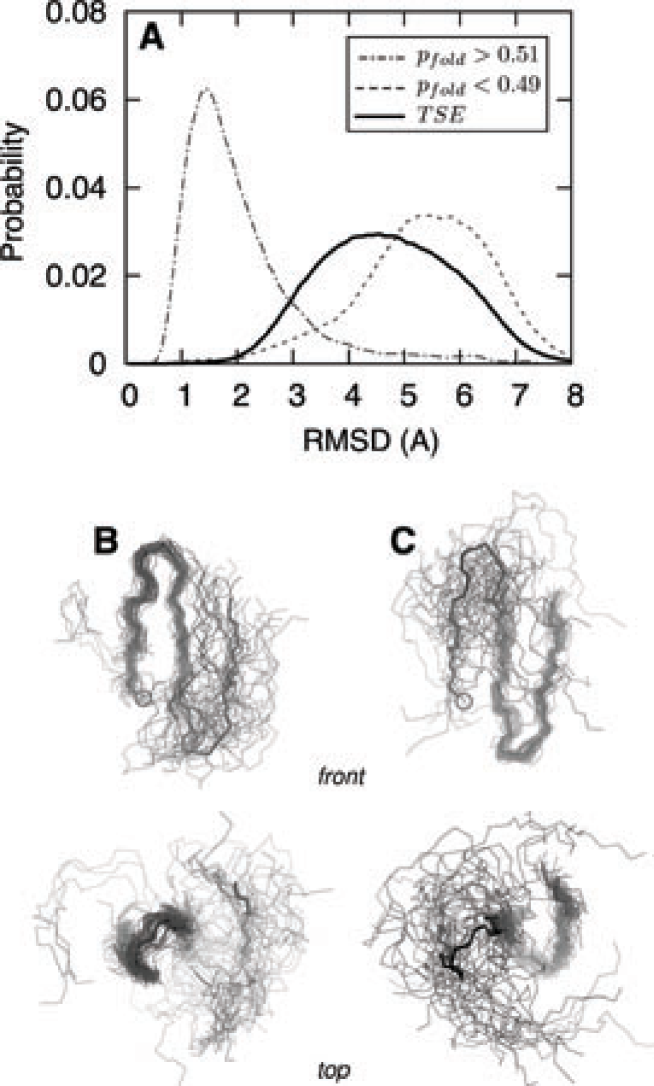
Figure 4: Transition state ensemble (TSE) of beta3s. (A) RMSD pairwise distribution for structures with $p_{fold}>0.51$ (native state), $0.49<p_{fold}<0.51$ (TSE), and $p_{fold}<0.49$ (denatured state). (B) Type I and (C) type II transition states (thin lines). Structures are superimposed on residues 2-11 and 10-19 with an average pairwise RMSD of 0.81 and 0.82 Å for type I and type II, respectively. For comparison, the native state is shown as a thick line with a circle to label the N-terminus.

The standard deviation of $p_{fold}$ in a cluster is computed as

$$\sigma_{p_{fold}}=\sqrt{\left<(p_{fold}(i)-P_{f}[\alpha])^{2}\right>_{i\in\alpha}}$$ (5)

In the case of full kinetic inhomogeneity, i.e., random grouping of snapshots, the $p_{fold}$ value for all snapshots in a given cluster will be equal to 0 or 1, indicating the coexistence (in the same cluster) of structures that either exclusively fold or unfold. In this case $\sigma_{p_{fold}}$ reflects the Bernoulli distribution (see Supp. Mat.). Fig. 2A shows that, even when only $n_{t}=10$ runs per snapshot are used to compute $p_{fold}$, $\sigma_{p_{fold}}$ values are not compatible with those of a Bernoulli distribution. Moreover the values of the standard deviation decrease when the number of trials $n_{t}$ increases, as reported in Fig. 2B for two sample clusters. The asymptotic value of $\sigma_{p_{fold}}$ ($n_{t}\rightarrow\infty$) for these two data sets is of 0.05 and 0.2. This value cannot reach zero because snapshots in a cluster are similar but not identical. These results suggest that snapshots inside the same cluster are kinetically homogeneous and a statistical description of $p_{fold}$ can be adopted, that is, folding probabilities are computed as cluster averages (instead of single snapshots) by means of $P_{f}$ and $P_{f}^{C}$.

We still have to verify that $P_{f}^{C}$ indeed approximates the computationally expensive $P_{f}$. Namely, for the 37 clusters mentioned above a correlation of 0.89 between $P_{f}^{C}$ and $P_{f}$ is found with a slope of 0.86 (see Fig. 3A and Tab. 1), indicating that the procedure is able to estimate folding probabilities for clusters on the folding-transition barrier ($P_{f}\sim 0.5$) as well as in the folding ($P_{f}\sim 1.0$) or unfolding ($P_{f}\sim 0.0$) regions. The error bars for $P_{f}^{C}$ in Fig. 3A are derived from the definition of variance given in Eq. 3. In the same spirit of Eq. 3 the folding probability $P_{f}$ and its variance are written as

$$\begin{split}P_{f}=&\left<\theta\right>=\frac{1}{N}\sum_{i=1}^{N}\theta_{i}\\ \sigma^{2}_{\left<\theta\right>}=&\frac{1}{N}P_{f}(1-P_{f})\end{split}$$ (6)

where $N=\sum n_{t}$ is the total number of runs and $\theta$ is equal to 1 or 0, if the run folded or unfolded, respectively. Note that the same number of runs $n_{t}$ has been used for every snapshot of a cluster. The large vertical error bars in Fig. 3A correspond to clusters with less than 10 snapshots. The largest deviations between $P_{f}$ and $P_{f}^{C}$ are around the $0.5$ region. This is due to the limited number of crossings of the folding barrier observed in the MD simulation (Fig. 3B, around 70 events of folding Cavalli et al. (2003)). Improvements in the accuracy for the estimation of $P_{f}$ are achieved as the number of folding events, i.e., the simulation time, increases (Fig. 3C-E).

The two main results of this study, i.e., the kinetic homogeneity of the clusters and the validity of $P_{f}^{C}$ as an approximation of $P_{f}$, are robust with respect to the choice of the clusterization. Similar results can be obtained also with different flavors of conformation space partitioning, as long as they group together structurally homogeneous conformations, e.g., clusterization based on root mean square deviation of atomic coordinates (RMSD) or secondary structure strings (see Supp. Mat.). The latter are appropriate for structured peptides but not for proteins with irregular secondary structure because of string degeneracy. Note that partitions based on order parameters (like native contacts) are usually unsatisfactory and not robust. This is mainly due to the fact that clusters defined in this way are characterized by large structural heterogeneities Rao and Caflisch (2004).

IV Analysis of transition state ensemble

The folding probability of structure $i$ is estimated as $p_{fold}(i)=P_{f}^{C}[\alpha]$ for $i\in\alpha$. This approximation allows to plot the pairwise RMSD distribution of beta3s structures with $p_{fold}>0.51$ (native state), $0.49<p_{fold}<0.51$ (transition state ensemble, TSE), and $p_{fold}<0.49$ (denatured state) (Fig. 4A). For the native state, the distribution is peaked around low values of RMSD ($\sim 1.5$ Å) indicating that structures with $p_{fold}>0.51$ are structurally similar and belong to a non-degenerate state. The statistical weight of this group of structures is 49.4% and corresponds to the expected statistics for the native state because the simulations are performed at the melting temperature. In the case of TSE, the distribution is broad because of the coexistence of heterogeneous structures. This scenario is compatible with the presence of multiple folding pathways. Beta3s folding was already shown to involve two main average pathways depending on the sequence of formation of the two hairpinsFerrara and Caflisch (2000); Rao and Caflisch (2004). Here, a naive approach based on the number of native contactsFerrara and Caflisch (2000) is used to structurally characterize the folding barrier. TSE structures with number of native contacts of the first hairpin greater than the ones of the second hairpin are called type I conformations (Fig. 4B), otherwise they are called type II (Fig. 4C). In both cases the transition state is characterized by the presence of one of the two native hairpins formed while the rest of the peptide is mainly unstructured. These findings are also in agreement with the complex network analysis of beta3s reported in Ref Rao and Caflisch, 2004. Finally, the denatured state shows a broad pairwise RMSD distribution around even larger values of RMSD ($\sim 5.5$ Å), indicating the presence of highly heterogeneous conformations.

V Conclusions

Two main results have emerged from the present study. First, snapshots grouped in structurally homogeneous clusters are characterized by similar values of $p_{fold}$. This result justifies the use of a statistical approach for the study of the kinetic properties of the structures sampled along a simulation. Second, given a set of structurally homogeneous clusters and a folding criterion, it is possible to obtain a first approximation of the folding probability for every structure sampled along an equilibrium folding-unfolding simulation. Thus, the cluster-$p_{fold}$ is a quantitative measure of the kinetic distance from the native state and is computationally very cheapCom . Furthermore, it can be used to detect multiple folding pathways. The accuracy in the identification of the transition state ensemble improves as the number of folding events observed in the simulation increases. Recently the cluster-$p_{fold}$ approach has been used to identify the transition state ensemble of a large set of beta3s mutants (for a total of 0.65 $ms$ of simulation timeSettanni et al. (2005)), which would have been impossible with traditional methods. As a further application, the cluster-$p_{fold}$ procedure can be used to validate TSE conformations obtained by wide-spread $G\bar{o}$ models.

I Secondary structure clusterization

Recently, the secondary structure has been used to cluster the conformation space of peptides (F. Rao et al, JMB 342, 299, 2004). Secondary structure along an MD simulation trajectory can be easily calculated using known algorithms (C.A.F. Andersen et al, Structure 10, 174, 2002). A cluster is a single string of secondary structure, e.g., the most populated conformation for beta3s is -EEEESSEEEEEESSEEEE- where ”E”, ”S”, and ”-” stand for extended, turn, and unstructured, respectively. There are 8 possible ”letters” in the secondary structure ”alphabet”: ”H”, ”G”, ”I”, ”E”, ”B”, ”T”, ”S”, and ”-”, standing for $\alpha$ helix, 3/10 helix, $\pi$ helix, extended, isolated $\beta$-bridge, hydrogen bonded turn, bend, and unstructured, respectively. Since the N- and C-terminal residues are always assigned an ”-” a 20-residue peptide can in principle assume $8^{18}\simeq 10^{16}$ conformations.

Figure S1: (left) $p_{fold}$ standard deviation inside a cluster for 16 secondary structure (sstr) and 37 DRMS 1.2 Å clusters. Both sstr and DRMS 1.2 Å clusterizations are defined by similar fluctuations. (right) Scatter plot of $P_{f}^{C}$ versus $P_{f}$ for sstr clusterization. In this case the folding criteria used is based on the native contacts $Q$ (Settanni et al., PNAS 102, 628, 2005). A folding (unfolding) event is realized when $Q>0.85$ ($Q<0.15$).

Figure S2: (top) Probability to have a given pairwise root mean square deviation (RMSD) inside a cluster for the secondary structure (sstr) and DRMS 1.2 Å clusterizations. (bottom) Probability to have a given variance for the RMSD inside a cluster. Both plots show that secondary structure clusters are less structurally homogeneous than DRMS 1.2 Å clusters.

II First passage times

The first passage time (fpt) to a given cluster $\alpha$ is computed as the time along the MD trajectory that any given snapshot takes to the first subsequent snapshot belonging to $\alpha$. In fig. S3 the fpt distribution to the folded state is shown for two different clusterizations of the conformation space. The double peak shape of the distribution provides evidence of the different time scales between intra-basin and inter-basin transitions. The wider shape of the intra-basin peak for the secondary structure clusterization is consistent with the higher degree of structural diversity with respect to the DRMS 1.2 Å clusterization (see previous section).

Figure S3: Probability distribution for the first passage times (fpt) to the most populated cluster (folded state). (top) DRMS 1.2 Å clusterization. (bottom) Secondary structure clusterization.

III Random clusterization

The results of this section were obtained using the DRMS 1.2 Å clusterization. In the text evidence was provided that the standard deviation of $p_{fold}$

$$\sigma_{p_{fold}}=\sqrt{\left<(p_{fold}(i)-P_{f}[\alpha])^{2}\right>_{i\in\alpha}}$$

is not compatible with the one of a Bernoulli distribution. This means that snapshots in a cluster have similar values of $p_{fold}$ and are kinetically homogeneous. This is not the case for a random clusterization of the snapshots. Since it is not feasible to compute the $p_{fold}$ for every snapshot of a simulation, the assumption that $p_{fold}$ of snapshot $i$ is equal to the cluster folding probability $P_{f}^{C}$ of its cluster (as computed in the text) is made. Then, snapshots are reshuffled in 50000 random clusters. The folding probability for a random cluster $\alpha_{R}$ is computed as $P_{f}=\left<p_{fold}\right>_{\alpha_{R}}$. Most of the snapshots will have $p_{fold}$ close to $1$ or $0$ (see Fig. 3B in the text) and because of the random grouping, i.e., no kinetic homogeneity, the above standard deviation $\sigma_{p_{fold}}$ resembles the one of a Bernoulli distribution as shown in Fig. S4. Data obtained from a DRMS 1.2 Å clusterization deviates from this behavior (compare Fig. 2A and Fig. S4). Moreover this deviation becomes bigger as the number of trials $n_{t}$, in this case $10$, increases (see Fig. 1B).

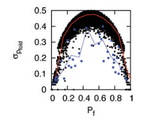
Figure S4: Standard deviation $\sigma_{p_{fold}}$ for a random clusterization. Black dots, red curve, blue squares, blue curve show $\sigma_{p_{fold}}$ for the random clusters, its histogram, $\sigma_{p_{fold}}$ for 37 non-random clusters (see text), and its histogram, respectively.