Role-similarity based functional prediction in networked systems:
Application to the yeast proteome

Abstract

We propose a general method to predict functions of vertices where: 1. The wiring of the network is somehow related to the vertex functionality. 2. A fraction of the vertices are functionally classified. The method is influenced by role-similarity measures of social network analysis. The two versions of our prediction scheme is tested on model networks were the functions of the vertices are designed to match their network surroundings. We also apply these methods to the proteome of the yeast Saccharomyces cerevisiae and find the results compatible with more specialized methods.

I Introduction

Systems made up of entities that interact pairwise can be modeled as networks. To comprehend the emergent properties of such systems—the objective of the study of complex systems and systems biology—one approach is to investigate the global properties of the corresponding networks mejn:rev ; ba:rev ; harary ; wf . In many cases the individual entities (or vertices) have distinct functions in the system. In such cases, provided the wiring of the edges relates to the function of vertices, one can predict these functions from the vertices’ position in the network. For example, a corporate hierarchy may be topped by a CEO, followed by a CFO and COO, so a chart of who reports to whom is enough to identify these positions. Another problem in this category of much recent interest is to predict protein functions hodg:pfp from the networks of protein interactions yook:protein ; deng:pfp ; hish:pfp ; leto:pfp ; sama:pfp ; vaz:pfp . These methods, like other methods based on e.g. protein sequences, are important because to confirm a protein function one needs function-specific and possibly hard-to-design in vivo, genetic or biochemical tests, while interaction and sequence data can be obtained fairly easily.

In this paper we propose a general method of predicting the functions of vertices in networked systems where the functions are partly mapped out. The rationale of our algorithm is to match unknown vertices with the most similar (judging from the network structure) categorized vertex and take the functions of the latter vertex as our forecast. The network similarity concept we ground our method on is related to the notion of regular equivalence eve:sim ; wf or role similarity regeeco1 of social network theory. Roughly speaking, two vertices are similar, in this sense, if the network looks alike from their respective perspectives. We evaluate our method on model networks where the categories of vertices reflect their placement in the network. We also apply the method to S. cerevisiae protein data obtained from the MIPS data base pagel:mips (data extracted January 23, 2005).

II Role similarity and definition of the prediction scheme

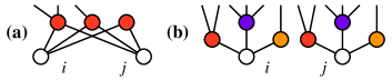
Figure 1: Illustration of structural and regular equivalence. $i$ and $j$ are structurally equivalent in (a) since they have the same neighborhoods, and regularly equivalent in (b) since there is a matching of regularly equivalent vertices between the neighborhoods. In (b) vertices of the same color are regularly equivalent.

Role similarity refers to rather broad set of concepts and related measures. Basically, the role of a vertex is determined by the characteristics of the vertices it is connected to wf . Consider two vertices $i$ and $j$. If their neighborhoods are similar, we say $i$ and $j$ have high role similarity. The question how to define the similarity of the neighborhoods $\Gamma_{i}$ and $\Gamma_{j}$ leads to two different concepts. One choice matches the identity of vertices in the neighborhood. This leads to the structural equivalence relation which is true if $\Gamma_{i}=\Gamma_{j}$. Another way to compare neighborhoods is to match the similarity of vertices in the neighborhood which gives the concept of regular equivalence—if one can pair the vertices of $\Gamma_{i}$ with vertices in $\Gamma_{j}$ such that each pair is regularly equivalent, then $i$ and $j$ are also regularly equivalent. Since vertices with the same functions need not, in general, be close, we will need a similarity score measuring how close to regular equivalence two vertices are. Following Refs. simrank ; blondel:sim we define a similarity score based on iterating the regular equivalence principle “two vertices are similar if they are pointed to, or point to, vertices that themselves similar.” In the general case of a directed network with $R$ different types of edges, one implementation of this argument is just to sum the similarities between vertices of the neighborhoods:

$$\sigma^{\mathrm{I}}_{n+1}(i,j)=\sum_{r=1}^{R}\left[\sum_{i^{\prime}\in\Gamma_{i,r}^{\mathrm{in}}}\sum_{j^{\prime}\in\Gamma_{j,r}^{\mathrm{in}}}\sigma^{\mathrm{I}}_{n}(i^{\prime},j^{\prime})+\sum_{i^{\prime}\in\Gamma_{i,r}^{\mathrm{out}}}\sum_{j^{\prime}\in\Gamma_{j,r}^{\mathrm{out}}}\sigma^{\mathrm{I}}_{n}(i^{\prime},j^{\prime})\right],$$ (1)

where $\sigma^{\mathrm{I}}_{n}(i,j)$ is the similarity between $i$ and $j$ after the $n$’th iteration and $\Gamma_{i,r}^{\mathrm{in}}$ is the in-neighborhood of $i$ with respect to $r$-edges. To avoid overflow problems we rescale all similarities so that $\max_{ij}|\sigma^{\mathrm{I}}_{n}(i,j)|=S$ after each iteration. We break the iteration when the sum, before the normalization, has not changed by more than a $10^{-8}$th of its previous value.

By the Eq. 1 definition, high degree vertices will appear more similar to the average other vertex than low-degree vertices. To compensate for this effect one may divide by the appropriate degrees (numbers of neighbors) to obtain:

$$\sigma^{\mathrm{II}}_{n+1}(i,j)=\sum_{r=1}^{R}\left[\frac{1}{k_{i,r}^{\mathrm{in}}\>k_{j,r}^{\mathrm{in}}}\sum_{i^{\prime}\in\Gamma_{i,r}^{\mathrm{in}}}\sum_{j^{\prime}\in\Gamma_{j,r}^{\mathrm{in}}}\sigma^{\mathrm{II}}_{n}(i^{\prime},j^{\prime})+\frac{1}{k_{i,r}^{\mathrm{out}}\>k_{j,r}^{\mathrm{out}}}\sum_{i^{\prime}\in\Gamma_{i,r}^{\mathrm{out}}}\sum_{j^{\prime}\in\Gamma_{j,r}^{\mathrm{out}}}\sigma^{\mathrm{II}}_{n}(i^{\prime},j^{\prime})\right],$$ (2)

where $k_{i,r}^{\mathrm{in}}$ is the in-degree of $i$ with respect to $r$-edges. From now on we call $\sigma^{\mathrm{I}}(i,j)=\sigma^{\mathrm{I}}_{\infty}(i,j)$ of Eq. 1 and $\sigma^{\mathrm{II}}(i,j)$ of Eq. 2 the I- and II-similarity between $i$ and $j$ respectively.

As mentioned, we suppose some of the vertices are functionally categorized. In general we assume one vertex can have many functions. For pairs of such functionally determined vertices the above similarities will add no information. Instead we define a functional similarity

$$\sigma_{f}(i,j)=J(F_{i},F_{j})-\langle J\rangle,$$ (3)

for such pairs, where $F_{i}$ is $i$’s function set (we assume a finite number of functions) and $J(\>\cdot\>)$ denotes the Jackard index $J(A,B)=|A\cap B|\>/\>|A\cup B|$ and the average is over all pairs of categorized vertices. We will later need $\sigma(i,j)=0$ to represent neutrality which is why we subtract the mean. Whenever a pair of classified vertices $(i,j)$ appears in the sums of Eqs. 1 or 2 we use the $\sigma_{f}(i,j)$ value of Eq. 3 instead of $\sigma^{\mathrm{I}}(i,j)$ or $\sigma^{\mathrm{II}}(i,j)$. I.e., we assume the functional classification is more accurate than the role-similarities and hence do not update the former.

In general we can now define our prediction scheme as follows:

1. For vertex pairs with at least one unclassified vertex initialize $\sigma_{0}(i,j)$ to $0$ if $i\neq j$ and to $1-\langle J\rangle$ otherwise.

2. Calculate the similarity scores for all pairs of unique vertices such that at least one is unclassified.

3. For an unclassified vertex $i$, predict the function set $F_{\hat{i}}$, where $\hat{i}$ is the classified vertex with highest similarity to $i$. If $\hat{i}$ is not unique, but a set $\hat{I}=\{\hat{i}_{1},\cdots,\hat{i}_{m}\}$ has the highest similarity to $i$, then let the set $G$ of functions present in more than half of the set of $j$’s be your guess. If $G$ is empty, let $F_{j}$ for a random $j\in\hat{I}$ be the guess.

The diagonal elements will have maximal functional similarity (which is why we set them to $1-\langle J\rangle$ in step 1), otherwise we assume neutrality. The backup selection rules in step 3 will typically be needed when unclassified vertices are structurally equivalent to classified vertices, the use of the majority rule instead of only a random guess will compensate for occasional errors in the assignment of functions to classified proteins. Our parameter $S$ sets the relative importance of the functional similarities to the subsequent assessments of $\sigma$. As mentioned above, the functional classification is assumed to be more accurate than the role-similarities, and it is thus sensible to choose a $\sigma\in[0,1-\langle J\rangle]$. The appropriate $S$ value is problem dependent. We will use $S=0{.}8$ which is in this interval for both our two test cases. To summarize, we have proposed two versions of our prediction scheme, scheme I and II, corresponding to I- and II-similarity.

III Application to model networks

To test our prediction algorithm we construct model networks where the assigned functions of the vertices correspond to their position in the network. We test the algorithm’s size scaling and performance in sub-ideal conditions by randomly perturbing the network.

III.1 Definition of the model networks

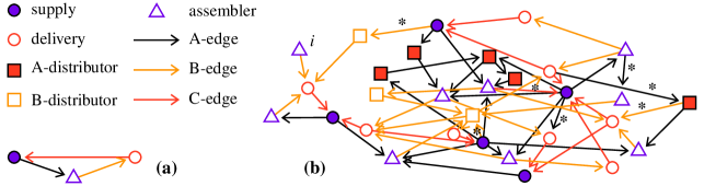
Figure 2: Model networks where vertex function and position are related. (a) shows the initial network. (b) shows a realization with 30 vertices and rewiring probability $r=0{.}1$. “*” indicates a rewired edge.

In defining our model, we will metaphorically use the flow of raw material, products and information in a manufacturing system. For our purpose we only need networks where the functions of vertices correspond to their position in their network surroundings—we will not further motivate its relevance as a model for manufacturing networks. We assign five distinct functional classes of the vertices: The supply vertices are the source of the raw material which flows along A-edges to assembler vertices. The assembled products are transported via B-edges to delivery vertices that dispatch the products. From the delivery vertices informational feedback is sent to the supply vertices through C-edges. Furthermore, the A and B-edges can fork at A- and B-distributor vertices.

The precise definition of the model is as follows: Start with the kernel shown in Fig. 2(a), then grow the network vertex by vertex. At each iteration, assign, with equal probability, one of the above functions to the new vertex. Then, depending on the assigned function, form edges including the new vertex as follows.

Supply.

Add an A-edge to an assembler or A-distributor, and a C-edge from a delivery vertex.

Assembly.

Add an A-edge from an assembler or A-distributor vertex, and a B-edge to an assembler or A-distributor.

Delivery.

Add a B-edge from an assembler or B-distributor, and a C-edge to a supplier.

A(B)-distribution.

Add an A(B)-edge from an assembler or A(B)-distributor vertex, and an A(B)-edge to an assembler or A(B)-distributor.

The choice of vertex to attach the new vertex to, given its functional category, is done with uniform randomness. Note that the number of edges will on average be twice the number of vertices (two edges are added per vertex).

From the definition so far, any vertex is identifiable from its neighborhood—a vertex with incoming C-edges and out-going A-edges is a supplier, and so on. Real data-sets are seldom perfect—neither in the wiring of the edges, nor in the functional classification. To test the prediction scheme under more realistic circumstances we randomize the network as follows: After generating a network according to the above scheme, we go through all edges sequentially. With a probability $r$ detach the from-side of an edge and re-attach it to a randomly chosen vertex such that no self-edge or multiple edge (of the same type—A, B or C) is formed. Rewire the to-side likewise with the same probability. A realization of the algorithm is displayed in Fig. 2(b). After the rewiring there is not necessarily enough information to classify a vertex—$i$ in Fig. 2(b) is an assembler but could just as well have been a B-distributor.

III.2 Prediction performance

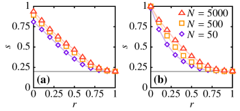
Figure 3: The fraction of correctly predicted functions $s$ for our model networks as a function of the rewiring probability $r$. (a) show the results based on I-similarities, (b) is the corresponding plot for II-similarities. The points are averaged over $\sim 1000$ runs of the network construction and prediction scheme with $a=1/50$. Errorbars are smaller than the symbol size. The horizontal line marks the limit of random guessing $0{.}2$.

To test the our prediction scheme we mark a random set of $aN$, $a\in(0,N)$, vertices unclassified. Then we predict the function of these vertices and let the average fraction of correctly predicted vertices $s$ be our performance measure. Fig. 3 shows $s$ for $a=1/50$ and different network sizes, as a function of the the rewiring probability $r$. In the small-$r$ limit the I-similarity prediction scheme makes an almost flawless job with $s>99{.}9\%$ for $N\geqslant 500$. Note, since we have five distinct functions, random guessing could not do better than $s=1/5$. This value, $s=1/5$, is by necessity attained in the random limit $r=1$. For small $r$-values the scheme II performs best, but if $r\lesssim 0{.}2$ scheme I performs slightly better. The size convergence for scheme I is faster, so in the large network limit II may outperform I. To understand the performance of the different schemes we note that scheme I has a tendency to match an unknown vertex to a known vertex of high degree. When $r=0$ this effect leads to some mispredictions for scheme I. But the redundant information about high degree vertices makes the more robust to minor perturbations, thus the slower decay of the $s(r)$-curves compared with scheme II.

We observe that the performance increases with the systems size for both schemes. This is important effect since databases in general grow in size–our prediction scheme will thus be more accurate with time. We surmise the explanation lies in, roughly speaking, that the bigger the network gets, the more likely it is that there is a very good matching. This is an effect local methods (taking only the surrounding of a vertex into account) could not utilize. A full explanation of this effect lies beyond the scope of this paper.

IV Predicting protein function in yeast

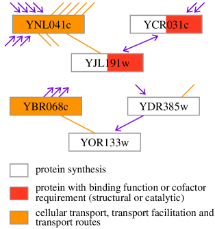
Figure 4: Example from the yeast protein prediction by scheme II on the first level functional data. When YJL191w is marked unknown it gets matched with YOR133w because their surroundings looks similar. The arrowed lines mark genetic regulation edges, other lines represent physical interaction.

IV.1 Functional prediction of proteins

Specifying protein functions experimentally requires demanding and potentially expensive tests. If one can obtain good guesses of the functions of an unknown protein, much is gained. During last decade, there has been a great number of methods suggested for protein functional prediction, including methods based on based on sequence or structure alignments paw:seq ; irving:struct , attributes derived from collections of sequences or structures jensen:seq ; dobson:struct , phylogenetic profiles pelle:pfp , or analysis of protein complexes gavin:complexes . Much of recent work has concentrated on functional prediction based on protein-protein interaction data. Many of these are specialized methods that exploit specific features of protein-protein interaction data vaz:pfp ; schw:pfp ; marc:pfp1 ; marc:pfp2 ; hodg:pfp ; leto:pfp ; sama:pfp (such as that vertices that interact physically are likely to share some functionality). The more general approaches deng:pfp ; hish:pfp are local in the sense that they are only based on pairwise statistics. For this reason they may not share the advantageous size scaling properties of our method.

IV.2 Applying the method to protein data

There are two types of large scale network data available for S. cerevisiae: “physical” and “genetic” protein-protein interactions. The terms “physical” and “genetic” refer to the type of experiment used to deduce the interaction. The genetic experiments are based on mutation studies, and the evidence from them is of a more indirect nature. We therefore distinguish between physical and genetic edges. All edges are undirected. Our data set, derived from the MIPS data base, has $N=4580$ linked together by $5129$ genetic regulation edges and $7434$ physical interaction edges. We removed duplicates, self-edges and interactions where one or both of the interacting substances were not proteins. The assigned functions are arranged in a hierarchical fashion, according to the FunCat categorization scheme ruepp:funcat used by the MIPS database. The first level contains the coarsest description of a protein’s function, such as “metabolism,” the second level is more specified e.g. “amino acid metabolism,” and so on. We will test our algorithm of the first and second level of this hierarchy and thus treat functions that differ in a finer classification as equal. There are three categories with no substantial functional information—“ubiquitous expression,” “classification not yet clear-cut” and “unclassified proteins.” We considered vertices with no other assigned categories than these three uncategorized.

In Fig. 4 we show a small example of scheme II in action on the yeast data. Suppose YJL191w is to be classified (we know it has the level-1 functions “protein with binding function …” and “protein synthesis”). The classified protein with highest similarity is YOR133w. This is because YNL041c, which interacts physically with YJL191w, is functionally identical (at level one of the hierarchy) to YBR068c that is physically linked to YOR133w. Similarly, YJL191w is genetically linked with YCR031c, which shares one functional category with YDR385w, which is genetically linked with YOR133w. These two features give a high similarity score to the pair YJL191w and YOR133w, so scheme II guesses that YJL191w has the functional category “protein synthesis” but misses the “protein with binding function …” category.

IV.3 Performance of the scheme

Table 1: The performance of our methods compared to the neighborhood counting method of Ref. schw:pfp . $s_{+}$ is the average fraction of correct predictions among the predicted functions averaged over all the classified proteins. $s_{-}$ is the average fraction of correct predictions among the actual functions.

	level 1			level 2
	NCM	Scheme I	Scheme II	NCM	Scheme I	Scheme II
$s_{+}$	0.269(6)	0.392(6)	0.337(6)	0.199(5)	0.238(6)	0.220(6)
$s_{-}$	0.354(6)	0.291(5)	0.346(7)	0.252(6)	0.199(5)	0.231(6)

For the previously described test networks we know a priori that the number of functions to be predicted is one. The same may be true for a variety of systems, but not for proteins. With the number of functions as one variable in the prediction problem we proceed to replace the success rate $s$ by the two measures precision $s_{+}$ and recall $s_{-}$ (the names borrowed from corresponding quantities in the text-mining literature, see e.g. Ref. rag:tm and references therein):

$$s_{+}=\left\langle\frac{n_{c}}{f_{*}}\right\rangle\mbox{~{}and~{}}s_{-}=\left\langle\frac{n_{c}}{f}\right\rangle,$$ (4)

where $n_{c}$ is the number of correctly predicted functions, $f$ is the real number of functions and $f_{*}$ is the number of predicted functions. $1-s_{+}$ is thus the expected fraction of false positive predictions (and similarly for $s_{-}$). Both these measures take values in the interval $[0,1]$ with $0$ meaning that no function is predicted correctly and $1$ represents perfect prediction. The averages are over the set of predicted functions in the same kind of leave-one-out estimates as performed for the test networks.

We follow Refs. vaz:pfp ; deng:pfp and use the neighborhood counting method (NCM) of Ref. schw:pfp for reference values. This method assigns the $f_{*}$ most frequent functions among the neighbors of the physical interaction network to the unknown protein. Considering its simplicity, compared with the more elaborate procedures listed above, this is a remarkably efficient method. (I.e., $f_{*}$ is a parameter of this model.) In our implementation, if the $f_{*}$’th function is not unique we select that randomly. Thus proteins with no neighbors are assigned $f_{*}$ functions randomly. Precision and recall values are displayed in Tab. 1. We use $f_{*}=2$ for the NCM which is the closest value to the average number of functions per protein for both levels one and two in our data set. The values may look low compared to similar tables in other papers on protein prediction, but these often do not include low-degree vertices, or use other performance measures (such as counting the fraction of proteins with at least one correctly predicted function, and so on). We note that, like the more disordered test networks, scheme II gives better performance in general (typically having better recall- but slightly worse precision-values).

V Summary and discussion

We have proposed methods for predicting the function of vertices in networked systems where the function of a vertex relates to its position. The principle behind our scheme is role equivalence as related to the regular equivalence concept of social network analysis. I.e., vertices are similar if the network, as seen from the respective vertices, look similar. We make two extensions to the method proposed in Refs. simrank ; blondel:sim to networks where some of the vertices are functionally categorized. The prediction of an uncategorized protein is then done by copying the functions of the other vertex with highest role similarity. Our schemes, corresponding to our two role similarities, are tested on model networks. These are designed to have a correspondence between the function of the vertex and their network surrounding. This correspondence can be tuned by a randomization parameter. We find that the performance of both schemes increases with the system size (the fraction of unknown vertices and rewired edges is fixed), which makes the applicability of our methods increasing with time (as data bases, in general, tend to grow). The differences between scheme I and II can be described by the fact that, scheme I gives (compared with scheme II) a higher similarity to vertex-pairs containing a high-degree vertex. Furthermore, we apply our method to the S. cerevisiae proteome. We use the networks of protein-protein interactions and obtain results that compare well with standard methods designed solely with protein functional prediction in mind. We do not claim that our method outperform the best specialized protein prediction methods—our aim is to construct a global method for general functional prediction, and most protein functional prediction schemes would perform poorly on our test networks. The ideas of this paper might however contribute to future, more elaborate, methods for prediction of protein functions.

The basic advantage of our method, as we see it, is that is a very general method that should apply to functional prediction in many systems. Moreover, it makes use of global network information, giving performance that does not decrease as the systems gets larger. The fact that it is a truly global algorithm—the prediction of every vertex’ functions takes wiring of the whole network into account—makes it rather slow (compared to e.g. specialized protein functional prediction methods, such as the one proposed in Ref. schw:pfp ). The execution time scales as $O(M^{2})$ (where $M$ is the total number of edges). But data sets of $10^{4}$-$10^{5}$, which cover e.g. the size of proteomes of known organisms, should be manageable to present day computers. We believe the problem of functional prediction in different types of networked systems is far from concluded—both in its full generality and the question how to utilize the characteristics of more specific systems.

Acknowledgments

The authors thank Micha Enevoldsen, Elizabeth Leicht and Mark Newman for comments.

References

- (1) Albert, R. & Barabási, A.-L. (2002) Rev. Mod. Phys. 74, 47–98.
- (2) Buckley, F. & Harary, F. (1989) Distance in graphs. (Addison-Wesley, Redwood City).
- (3) Newman, M. E. J. (2003) SIAM Rev. 45, 167–256.
- (4) Wasserman, S. & Faust, K. (1994) Social network analysis: Methods and applications. (Cambridge University Press, Cambridge).
- (5) Hodgman, T. (2000) Bioinformatics 16, 10–15.
- (6) Yook, S., Oltvai, Z. & Barabási, A.-L. (2004) Proteomics 4, 928–942.
- (7) Samanta, M. P. & Liang, S. (2003) Proc. Natl. Acad. Sci. USA 100, 12579–12583.
- (8) Vazquez, A., Flammini, A., Martian, A., & Vespignani, A. (2003) Nature Biotech. 21, 697–700.
- (9) Deng, M., Zhang, K., Mehta, S., Chen, T. & Sun, F. (2002) in Proceedings of the IEEE Computer Society Bioinformatics Conference (CSB 02). (Stanford CA), pp. 197–207.
- (10) Hishigaki, H., Nakai, K., Ono, T., Tanigami, A. & Tagaki, T. (2001) Yeast 18, 523–531.
- (11) Letovsky, S. & Kasif, S. (2003) Bioinformatics 19, 197–204.
- (12) Everett, M. G. (1985) Soc. Netw. 7, 353–359.
- (13) Luczkovich, J. J., Borgatti, S. P., Johnson, J. C., & Everett, M. G. (2003) J. Theor. Biol. 220, 303–321.
- (14) Pagel, P., Kovac, S., Oesterheld, M., Brauner, B., Dunger-Kaltenbach, I., Frishman, G., Montrone, C., Mark, P., Stümpflen, V., Mewes, H. W. et al. (2004) Bioinformatics, [Epub ahead of print] doi:10.1093/bioinformatics/bti115.
- (15) Guimerà, R. & Nunes Amaral, L. A. (2005) Nature 433, 895–900.
- (16) Lusseau, D. & Newman, M. E. J. (2004) Proc. R. Soc. London B 271, 477–481.
- (17) Blondel, V. D., Gajardo, A., Heymans, M., Senellart, P., & van Dooren, P. (2004) SIAM Rev. 46, 647–666.
- (18) Jeh, G. & Widom, J. (2002) Proceedings of the eighth ACM SIGKDD international conference on knowledge discovery and data mining. (Edmonton), pp. 538–543.
- (19) Pawlowski, K., Jaroszewski, L., Rychlewski, L. & Godzik, A. (2000) Pac. Symp. Biocomput., 42–53.
- (20) Irving, J. A., Whisstock, J. C. & Lesk, A. M. (2001) Proteins 42, 378–382.
- (21) Jensen, L. J., Staerfeldt, H. & Brunak, S. (2003) Bioinformatics 19, 635–642.
- (22) Dobson, P. D. & Doig, A. S. (2003) J. Mol. Biol. 330, 771–783.
- (23) Pellegrini, M., Marcotte, E., Thompson, M. J., Eisenberg, D. & Yeates, T. O. (1999) Proc. Natl. Acad. Sci. USA 96, 4285–4288.
- (24) Gavin, A. C., Bosche, M., Krause, R., Grandi, P., Marzioch, M., Bauer, A., Schultz, J., Rick, J. M., Michon, A. M., Cruciat, C. M., Remor, M. et al. (2004) Nucleic Acids Res. 32, 5539–5545.
- (25) Marcotte, E. M., Pellegrini, M., Ng, H. L., Rice, D. W., Yeates, T. O. & Eisenberg, D. (1999) Science 285, 751–753.
- (26) Marcotte, E. M., Pellegrini, M., Thompson, M. J., Yeates, T. O. & Eisenberg, D. (1999) Nature 402, 83–86.
- (27) Schwikowski, B., Uetz, P. & Fields, S. (2000) Nature Biotech. 18, 1257–1261.
- (28) Ruepp, A., Zollner, A., Albermann, K., Hani, J., Mokrejs, M., Tetko, I., Guldener, U., Mannhaupt, G., Munsterkotter, M. & Mewes, H. W. (2004) Nucleic Acids Res. 32, 5539–5545.
- (29) Raghavan, V. V., Jung G. S. & Bollmann, P. (1989) ACM Trans. Inf. Syst. 7, 205–229.