The Basic Reproductive Number of Ebola and the Effects of Public Health Measures: The Cases of Congo and Uganda

Abstract

Despite improved control measures, Ebola remains a serious public health risk in African regions where recurrent outbreaks have been observed since the initial epidemic in $1976$. Using epidemic modeling and data from two well-documented Ebola outbreaks (Congo $1995$ and Uganda $2000$), we estimate the number of secondary cases generated by an index case in the absence of control interventions ($R_{0}$). Our estimate of $R_{0}$ is $1.83$ (SD $0.06$) for Congo (1995) and $1.34$ (SD $0.03$) for Uganda (2000). We model the course of the outbreaks via an SEIR (susceptible-exposed-infectious-removed) epidemic model that includes a smooth transition in the transmission rate after control interventions are put in place. We perform an uncertainty analysis of the basic reproductive number $R_{0}$ to quantify its sensitivity to other disease-related parameters. We also analyze the sensitivity of the final epidemic size to the time interventions begin and provide a distribution for the final epidemic size. The control measures implemented during these two outbreaks (including education and contact tracing followed by quarantine) reduce the final epidemic size by a factor of $2$ relative the final size with a two-week delay in their implementation.

1 Introduction

Ebola hemorrhagic fever is a highly infectious and lethal disease named after a river in the Democratic Republic of the Congo (formerly Zaire) where it was first identified in 1976 [1]. Twelve outbreaks of Ebola have been reported in Congo, Sudan, Gabon, and Uganda as of September 14, 2003 [2, 3]. Two different strains of the Ebola virus (Ebola-Zaire and the Ebola-Sudan) have been reported in those regions. Despite extensive search, the reservoir of the Ebola virus has not yet been identified [4, 5]. Ebola is transmitted by physical contact with body fluids, secretions, tissues or semen from infected persons [1, 6]. Nosocomial transmission (transmission from patients within hospital settings) has been typical as patients are often treated by unprepared hospital personnel (barrier nursing techniques need to be observed). Individuals exposed to the virus who become infectious do so after a mean incubation period of $6.3$ days ($1-21$ days) [7]. Ebola is characterized by initial flu-like symptoms which rapidly progress to vomiting, diarrhea, rash, and internal and external bleeding. Infected individuals receive limited care as no specific treatment or vaccine exists. Most infected persons die within $10$ days of their initial infection [8] ($50\%-90\%$ mortality [6]).

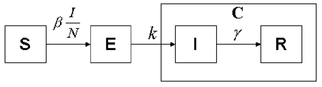
Figure 1: A schematic representation of the flow of individuals between epidemiological classes. $\beta\frac{I}{N}$ is the transmission rate to susceptibles $S$ from $I$; $E$ is the class of infected (not yet infectious) individuals; $k$ is the rate at which $E$-individuals move to the symptomatic and infectious class $I$; Infectious individuals ($I$) either die or recover at rate $\gamma$. $C$ is not an epidemiological state but keeps track of the cumulative number of cases after the time of onset of symptoms.

Using a simple SEIR (susceptible-exposed-infectious-removed) epidemic model (Figure 1) and data from two well-documented Ebola outbreaks (Congo $1995$ and Uganda $2000$), we estimate the number of secondary cases generated by an index case in the absence of control interventions ($R_{0}$). Our estimates of $R_{0}$ are $1.83$ (SD $0.06$) for Congo (1995) and $1.34$ (SD $0.03$) for Uganda (2000). We model the course of the outbreaks via an SEIR epidemic model that includes a smooth transition in the transmission rate after control interventions are put in place. We also perform an uncertainty analysis on the basic reproductive number $R_{0}$ to account for its sensitivity to disease-related parameters and analyze the model sensitivity of the final epidemic size to the time at which interventions begin. We provide a distribution for the final epidemic size. A two-week delay in implementing public health measures results in an approximated doubling of the final epidemic size.

2 Methods

We fit data from Ebola hemorrhagic fever outbreaks in Congo (1995) and Uganda (2000) to a simple deterministic (continuous time) SEIR epidemic model (Figure 1). The least-squares fit of the model provides estimates for the epidemic parameters. The fitted model can then be used to estimate the basic reproductive number $R_{0}$ and quantify the impact of intervention measures on the transmission rate of the disease. Interpreting the fitted model as an expected value of a Markov process, we use multiple stochastic realizations of the epidemic to estimate a distribution for the final epidemic size. We also study the sensitivity of the final epidemic size to the timing of interventions and perform an uncertainty analysis on $R_{0}$ to account for the high variability in disease-related parameters in our model.

2.1 Epidemic Models

Individuals are assumed to be in one of the following epidemiological states (Figure 1): susceptibles (at risk of contracting the disease), exposed (infected but not yet infectious), infectives (capable of transmitting the disease), and removed (those who recover or die from the disease).

2.1.1 Differential Equation Model

Susceptible individuals in class $S$ in contact with the virus enter the exposed class $E$ at the per-capita rate $\beta I/N$, where $\beta$ is transmission rate per person per day, $N$ is the total effective population size, and $I/N$ is the probability that a contact is made with a infectious individual (i.e. uniform mixing is assumed). Exposed individuals undergo an average incubation period (assumed asymptomatic and uninfectious) of $1/k$ days before progressing to the infectious class $I$. Infectious individuals move to the $R$-class (death or recovered) at the per-capita rate $\gamma$ (see Figure 1). The above transmission process is modeled by the following system of nonlinear ordinary differential equations [9, 10]:

$$\begin{array}[]{rcl}{\displaystyle\dot{S}(t)}&=&-\beta S(t)I(t)/N\\ {\displaystyle\dot{E}(t)}&=&\beta S(t)I(t)/N-kE(t)\\ {\displaystyle\dot{I}(t)}&=&kE(t)-\gamma I(t)\\ {\displaystyle\dot{R}(t)}&=&\gamma I(t)\\ {\displaystyle\dot{C}(t)}&=&kE(t),\\ \end{array}$$ (1)

where $S(t)$, $E(t)$, $I(t)$, and $R(t)$ denote the number of susceptible, exposed, infectious, and removed individuals at time $t$ (the dot denotes time derivatives). $C(t)$ is not an epidemiological state but serves to keep track of the cumulative number of Ebola cases from the time of onset of symptoms.

2.1.2 Markov Chain Model

The analogous stochastic model (continuous time Markov chain) is constructed by considering three events: exposure, infection and removal. The transition rates are defined as:

Event	Effect	Transition rate
Exposure	(S, E, I, R)  $\rightarrow$  (S-1, E+1, I, R)	$\beta(t)SI/N$
Infection	(S, E, I, R)  $\rightarrow$  (S, E-1, I+1, R)	$kE$
Removal	(S, E, I, R)  $\rightarrow$  (S, E, I-1, R+1)	$\gamma I$

The event times $0<T_{1}<T_{2}<...$ at which an individual moves from one state to another are modeled as a renewal process with increments distributed exponentially,

$$P(T_{k}-T_{k-1}>t|T_{j},j\leq k-1)=e^{-t\mu(T_{k-1})}$$

where $\mu(T_{k-1})=(\beta(T_{k-1})S(T_{k-1})I(T_{k-1})/N+kE(T_{k-1})+\gamma I(T_{k-1}))^{-1}$.

The final epidemic size is $Z=C(T)$ where $T=min\{t>0,E(t)+I(t)=0\}$, and its empirical distribution can be computed via Monte Carlo simulations [11].

2.2 The Transmission Rate and the Impact of Interventions

The intervention strategies to control the spread of Ebola include surveillance, placement of suspected cases in quarantine for three weeks (the maximum estimated length of the incubation period), education of hospital personnel and community members on the use of strict barrier nursing techniques (i.e protective clothing and equipment, patient management), and the rapid burial or cremation of patients who die from the disease [6]. Their net effect, in our model, is to reduce the transmission rate $\beta$ from $\beta_{0}$ to $\beta_{1}<\beta_{0}$. In practice, the impact of the intervention is not instantaneous. Between the time of the onset of the intervention to the time of full compliance, the transmission rate is assumed to decrease gradually from $\beta_{0}$ to $\beta_{1}$ according to

$$\beta(t)=\left\{\begin{array}[]{ll}\beta_{0}&t<\tau\\ \beta_{1}+(\beta_{0}-\beta_{1})e^{-q(t-\tau)}&t\geq\tau\end{array}\right.$$

where $\tau$ is the time at which interventions start and $q$ controls the rate of the transition from $\beta_{0}$ to $\beta_{1}$. Another interpretation of the parameter $q$ can be given in terms of $t_{h}=\frac{ln(2)}{q}$, the time to achieve $\beta(t)=\frac{\beta_{0}+\beta_{1}}{2}$.

2.3 Epidemiological data

The data for the Congo (1995) and Uganda (2000) Ebola hemorrhagic fever outbreaks include the identification dates of the causative agent and data sources. The reported data are ($t_{i}$, $y_{i}$), $i=1,...,n$ where $t_{i}$ denotes the $i^{th}$ reporting time and $y_{i}$ the cumulative number of infectious cases from the beginning of the outbreak to time $t_{i}$.

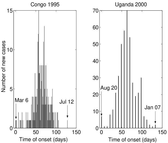
Figure 2: On the left, we have the daily number of cases by date of symptom onset during the Ebola outbreak in Congo 1995 (Mar $6$-Jul $12$). On the right, we have the weekly number of cases by date of symptom onset during the Ebola outbreak in Uganda $2000$ (Aug $20$-Jan $07$). Data has been taken from refs. [12, 13].

Congo 1995. This outbreak began in the Bandundu region, primarily in Kikwit, located on the banks of the Kwilu River. The first case (January 6) involved a 42-year old male charcoal worker and farmer who died on January 13. The Ebola virus was not identified as the causative agent until May $9$. At that time, an international team implemented a control plan that involved active surveillance (identification of cases) and education programs for infected people and their family members. Family members were visited for up to three weeks (maximum incubation period) after their last identified contact with a probable case. Nosocomial transmission occurred in Kikwit General Hospital but it was halted through the institution of strict barrier nursing techniques that included the use of protective equipment and special isolation wards. A total of $315$ cases of Ebola were identified ($81\%$ case fatality). Daily Ebola cases by date of symptom onset from March $1$ through July $12$ are available (Figure 2) [12].

Uganda 2000. A total of $425$ cases ($53\%$ case fatality) of Ebola were identified in three districts of Uganda: Gulu, Masindi and Mbara. The onset of symptoms for the first reported case was on August $30$, but the cause was not identified as Ebola until October $15$ by the National Institute of Virology in Johannesburg (South Africa). Active surveillance started during the third week of October. A plan that included the voluntary hospitalization of probable cases was then put in place. Suspected cases were closely followed for up to three weeks. Other control measures included community education (avoiding crowd gatherings during burials) and the systematic implementation of protective measures by health care personnel and the use of special isolation wards in hospitals. Weekly Ebola cases by date of symptom onset are available from the WHO (World Health Organization) [13] (from August $20$, $2000$ through January $7$, $2001$) (Figure 2).

2.4 Parameter Estimation

Empirical studies in Congo suggest that the incubation period is less than $21$ days with a mean of $6.3$ days [7] and the infectious period is between $3.5$ and $10.7$ days. The model parameters $\Theta=(\beta_{0}$, $\beta_{1}$, $k$, $q$, $\gamma$) are fitted to the Congo (1995) and Uganda (2000) Ebola outbreak data by least squares fit to the cumulative number of cases $C(t,\Theta)$ in eqn. (1). We used a computer program (Berkeley Madonna, Berkeley, CA) and appropriate initial conditions for the parameters ($0<\beta<1$, $0<q<100$, $1<1/k<21$ [7], $3.5<1/\gamma<10.7$ [14]). The optimization process was repeated $10$ times (each time the program is fed with two different initial conditions for each parameter) before the “best fit” was chosen. The asymptotic variance-covariance $AV(\hat{\theta})$ of the least-squares estimate is

$$AV(\hat{\theta})=\sigma^{2}(\sum^{n}_{i=1}\nabla C(t_{i},\Theta_{0})\nabla C(t_{i},\Theta_{0})^{T})^{-1}$$

which we estimate by

$$\hat{\sigma}^{2}(\sum_{i=1}^{n}\hat{\nabla C}(t_{i},\hat{\Theta})\hat{\nabla C}(t_{i},\hat{\Theta})^{T})^{-1}$$

where $n$ is the total number of observations, $\hat{\sigma}^{2}=\frac{1}{n-5}\sum(y_{i}-C(t_{i},\hat{\Theta}))^{2}$ and $\hat{\nabla C}$ are numerical derivatives of $C$.

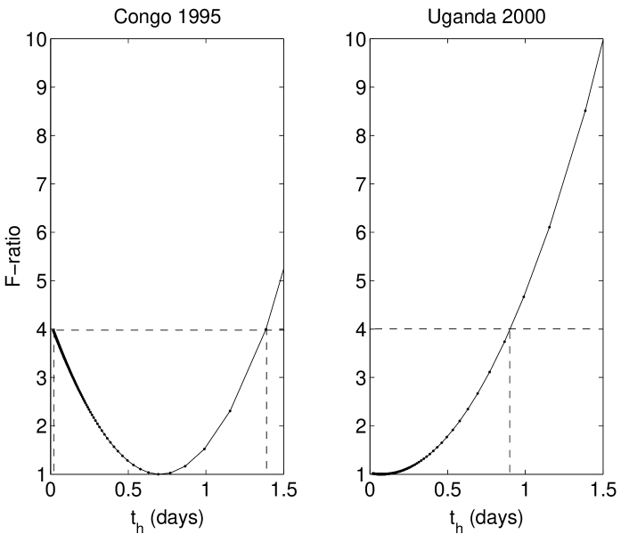
Figure 3: $95\%$ confidence intervals for $t_{h}$ ($t_{h}=\frac{log(2)}{q}$), the time to achieve a transmission rate of $\frac{\beta_{0}+\beta_{1}}{2}$, obtained from the likelihood ratio as described in the text.

For small samples, the confidence intervals based on these variance estimates may not have the nominal coverage probability. For example, for the case of Zaire $1995$, the $95\%$ confidence interval for $q$ based on asymptomatic normality is ($-0.26,2.22$). It should be obvious that this interval is not “sharp” as it covers negative values whereas we know $q\geq 0$. The likelihood ratio provides an attractive alternative to build confidence sets (Figure 3). Formally, these sets are of the form

$$\left\{\Theta:\frac{\sum(y_{i}-C(t_{i},\Theta))^{2}}{\sum(y_{i}-C(t_{i},\hat{\Theta}))^{2}}\leq A_{\alpha}\right\}$$

where $A_{\alpha}$ is the $1-\alpha$ quantile of an $F$ distribution with appropriate degrees of freedom. Parameter estimates are given in Table 1.

2.5 The Reproductive Number

The basic reproductive number $R_{0}$ measures the average number of secondary cases generated by a primary case in a pool of mostly susceptible individuals [9, 10] and is an estimate of the epidemic growth at the start of an outbreak if everyone is susceptible. That is, a primary case generates $R_{0}=\frac{\beta_{0}}{\gamma}$ new cases on the average where $\beta_{0}$ is the pre-interventions transmission rate and $1/\gamma$ is the mean infectious period. The effective reproductive number at time $t$, $R_{eff}(t)=\frac{\beta(t)}{\gamma}x(t)$, measures the average number of secondary cases per infectious case $t$ time units after the introduction of the initial infections and $x(t)=\frac{S(t)}{N}\approx 1$ as the population size is much larger than the resulting size of the outbreak (Table 2). Hence, $R_{eff}(0)=R_{0}$. In a closed population, the effective reproductive number $R_{eff}(t)$ is non-increasing as the size of the susceptible population decreases. The case $R_{eff}(t)\leq 1$ is of special interest as it highlights the crossing of the threshold to eventual control of the outbreak. An intervention is judged successful if it reduces the effective reproductive number to a value less than one. In our model, the post-intevention reproductive number $R_{p}=\frac{\beta_{1}}{\gamma}$ where $\beta_{1}$ denotes the post-intervention transmission rate. In general, the smaller $\beta_{1}$, the faster an outbreak is extinguished. By the delta method [15], the variance of the estimated basic reproductive number $\hat{R_{0}}$ is approximately

$$V(\hat{R_{0}})\approx\hat{R_{0}}^{2}\ \{\frac{V(\hat{\beta_{0}})}{\hat{\beta_{0}}^{2}}+\frac{V(\hat{\gamma})}{\hat{\gamma}^{2}}-\frac{2Cov(\hat{\beta_{0}},\hat{\gamma})}{\hat{\beta_{0}}\hat{\gamma}}\}.$$

2.6 The Effective Population Size

A rough estimate of the population size in the Bandundu region of Congo (where the epidemic developed) in 1995 is computed from the population size of the Bandundu region in $1984$ [16] and annual population growth rates [17] (Table 2). For the case of Uganda (2000), we adjusted the population sizes of the districts of Gulu, Masindi and Mbara in $1991$ and annual population growth rates [18] (Table 2). These estimates are an upper bound of the effective population size (those at risk of becoming infected) for each region. Estimates of the effective population size are essential when the incidence is modeled with the pseudo mass-action assumption ($\beta(t)SI$) which implies that transmission grows linearly with the population size and hence the basic reproductive number $R_{0}(N)=\beta_{0}N/\gamma$. In our model, we use the true mass-action assumption ($\beta(t)SI/N$) which makes the model parameters (homogeneous system of order $1$) independent of $N$ and hence the basic reproductive number can be estimated by $R_{0}=\beta_{0}/\gamma$ [19]. In fact, comparisons between the pseudo mass-action and the true mass-action assumptions with experimental data have concluded in favor of the later [20]. The model assumption that $N$ is constant is not critical as the outbreaks resulted in a small number of cases compared to the size of the population.

2.7 Uncertainty Analysis on $R_{0}$

Log-normal distributions seem to model well the incubation period distributions for a large number of diseases [21]. Here, a log-normal distribution is assumed for the incubation period of Ebola in our uncertainty analysis. Log-normal distribution parameters are set from empirical observations (mean incubation period is $6.3$ and the $95\%$ quantile is $21$ days [7]). The infectious period is assumed to be uniformly distributed in the range ($3.5-10.7$) days [14].

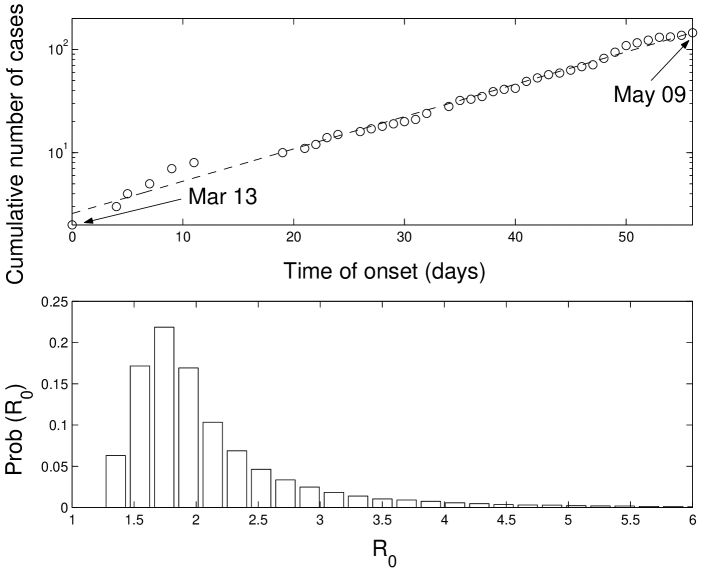
Figure 4: (Top) cumulative number of cases (log-lin scale) during the exponential growth phase of the Congo $1995$ epidemic as identified by the date of start of interventions ($09$ May $1995$ [12]). The model-free initial growth rate of the number of cases for Congo 1995 is $0.07$ (linear regression); (bottom) estimated distribution of $R_{0}$ from our uncertainty analysis (see text). $R_{0}$ lies in the interquartile range (IQR) ($1.66-2.28$) with a median of $1.89$. Notice that $100\%$ of the weight lies above $R_{0}=1$.

A formula for the basic reproductive number $R_{0}$ that depends on the initial per-capita rate of growth $r$ in the number of cases (Figure 4), the incubation period ($1/k$) and the infectious period ($1/\gamma$) can be obtained by linearizing equations $\dot{E}$ and $\dot{I}$ of system (1) around the disease-free equilibrium with $S=N$. The corresponding Jacobian matrix is given by:

$$J=\left(\begin{array}[]{cc}-k&\beta\\ k&-\gamma\\ \end{array}\right),$$

and the characteristic equation is given by:

$$r^{2}+(k+\gamma)r+(\gamma-\beta)k=0$$

where the early-time and per-capita free growth $r$ is essentially the dominant eigenvalue. By solving for $\beta$ in terms of $r$, $k$ and $\gamma$, one can obtain the following expression for $R_{0}$ using the fact that $R_{0}=\beta/\gamma$:

$${R_{0}}=1+\frac{r^{2}+(k+\gamma)r}{k\gamma}.$$

Our estimate of the initial rate of growth $r$ for the Congo 1995 epidemic is $r=0.07$ day^-1, obtained from the time series $y(t)$, $t<\tau$ of the cumulative number of cases and assuming exponential growth ($y(t)\propto e^{rt}$). The distribution of $R_{0}$ (Figure 4) lies in the interquartile range (IQR) ($1.66-2.28$) with a median of $1.89$, generated from Monte Carlo sampling of size $10^{5}$ from the distributed epidemic parameters ($1/k$ and $1/\gamma$) for fixed $r$ [22]. We give the median of $R_{0}$ (not the mean) as the resulting distribution of $R_{0}$ from our uncertainty analysis is skewed to the right.

3 Results

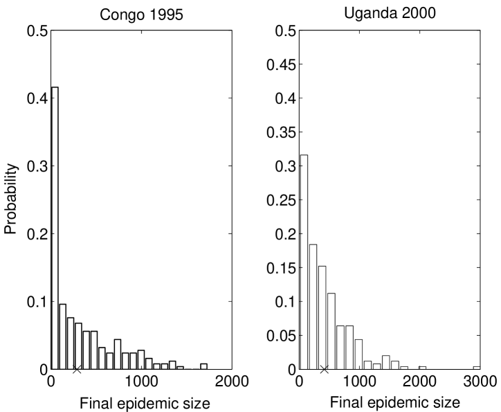
Figure 6: The final epidemic size distributions for the cases of Congo $1995$ and Uganda $2000$ obtained from $250$ Monte Carlo replicas. Crosses (X) represent the final epidemic size from data.

Using our parameter estimates (Table 1), we estimate an $R_{0}$ of $1.83$ (SD $0.06$) for Congo (1995) and $1.34$ (SD $0.03$) for Uganda (2000). The effectiveness of interventions is often quantified in terms of the reproductive number $R_{p}$ after interventions are put in place. For the case of Congo $R_{p}=0.51$ (SD $0.04$) and $R_{p}=0.66$ (SD $0.02$) for Uganda allowing us to conclude that in both cases, the intervention was successful in controlling the epidemic. Furthermore, the time to achieve a transmission rate of $\frac{\beta_{0}+\beta_{1}}{2}$ ($t_{h}$) is $0.71$ ($95\%$ CI ($0.02,1.39$)) days and $0.11$ ($95\%$ CI ($0,0.87$)) days for the cases of Congo and Uganda respectively after the time at which interventions begin.
We use the estimated parameters to simulate the Ebola outbreaks in Congo (1995) and Uganda (2000) via Monte Carlo simulations of the stochastic model of Section $2.1$ [11]. There is very good agreement between the mean of the stochastic simulations and the reported cases despite the “wiggle” captured in the residuals around the time $\tau$ of the start of interventions (Figure 5). The empirical distribution of the final epidemic sizes for the cases of Congo $1995$ and Uganda $2000$ are given in Figure 6.
The final epidemic size is sensitive to the start time of interventions $\tau$. Numerical solutions (deterministic model) show that the final epidemic size grows exponentially fast with the initial time of interventions (not surprising as the intial epidemic growth is driven by exponential dynamics). For instance, for the case of Congo, our model predicts that there would have been $20$ more cases if interventions had started one day later (Figure 7).

4 Discussion

Using epidemic-curve data from two major Ebola hemorrhagic fever outbreaks [12, 13], we have estimated the basic reproductive number ($R_{0}$) (Table 2). Our estimate of $R_{0}$ (median is $1.89$) obtained from an uncertainty analysis [22] by simple random sampling (Figure 4) of the parameters $k$ and $\gamma$ distributed according to empirical data from the Zaire (now the Democratic Republic of Congo) $1976$ Ebola outbreak [7, 14] is in agreement with our estimate of $R_{0}=1.83$ from the outbreak in Congo $1995$ (obtained from least squares fitting of our model (1) to epidemic curve data).
The difference in the basic reproductive numbers $R_{0}$ between Congo and Uganda is due to our different estimates for the infectious period ($1/\gamma$) observed in these two places. Their transmission rates $\beta_{0}$ are quite similar (Table 1). Our estimate for the infectious period for the case of Congo ($5.61$ days) is slightly larger than that of Uganda ($3.50$ days). Clearly, a larger infectious period increases the likelihood of infecting a susceptible individual and hence increases the basic reproductive number. The difference in the infectious periods might be due to differences in virus subtypes [23]. The Congo outbreak was caused by the Ebola-Zaire virus subtype [12] while the Uganda outbreak was caused by the Ebola-Sudan virus subtype [13].
The significant reduction from the basic reproductive number ($R_{0}$) to the post-intervention reproductive number ($R_{p}$) in our estimates for Congo and Uganda shows that the implementation of control measures such as education, contact tracing and quarantine will have a significant effect on lowering the effective reproductive rate of Ebola. Furthermore, estimates for the time to achieve $\frac{\beta_{0}+\beta_{1}}{2}$ have been provided (Table 1).
We have explored the sensitivity of the final epidemic size to the starting time of interventions. The exponential increase of the final epidemic size with the time of start of interventions (Figure 7) supports the idea that the rapid implementation of control measures should be considered as a critical component in any contingency plan against disease outbreaks specially for those like Ebola and SARS for which no specific treatment or vaccine exists. A two-week delay in implementing public health measures results in an approximated doubling of the final outbreak size. Because the existing control measures cut the transmission rate to less than half, we should seek and support further improvement in the effectiveness of interventions for Ebola. A mathematical model that considers basic public health interventions for SARS control in Toronto supports this conclusion [24, 25]. Moreover, computer simulations show that small perturbations to the rate $q$ at which interventions are put fully in place do not have a significant effect on the final epidemic size. The rapid identification of an outbreak, of course, remains the strongest determinant of the final outbreak size.
Field studies of Ebola virus are difficult to conduct due to the high risk imposed on the scientific and medical personnel [26]. Recently, a new vaccine that makes use of an adenovirus technology has been shown to give cynomolgus macaques protection within $4$ weeks of a single jab [27, 28]. If the vaccine turns out to be effective in humans, then its value should be tested. A key question would be “What are the conditions for a successful target vaccination campaign during an Ebola outbreak?” To address questions of this type elaborate models need to be developed.

Tables & Figures

		Congo 1995		Uganda 2000
Parameter	Definition	Estim.	S. D.	Estim.	S.  D.
$\beta_{0}$	Pre-interventions transmission rate (days-1)	$0.33$	$0.06$	$0.38$	$0.24$
$\beta_{1}$	Post-interventions transmission rate (days-1)	$0.09$	$0.01$	$0.19$	$0.13$
$t_{h}$	Time to achieve $\frac{\beta_{0}+\beta_{1}}{2}$ (days)	$0.71$	$(0.02,1.39)$	$0.11$	$(0,0.87)$
$1/k$	Mean incubation period (days)	$5.30$	$0.23$	$3.35$	$0.49$
$1/\gamma$	Mean infectious period (days)	$5.61$	$0.19$	$3.50$	$0.67$

Table 1: Parameter definitions and baseline estimates obtained from the best fit of the model equations (1) to the epidemic-curve data of the Congo $1995$ and Uganda $2000$ outbreaks (Figure 5). The parameters were optimized by a computer program (Berkeley Madonna, Berkeley, CA) using a least squares fitting technique and appropriate initial conditions for the parameters ($0<\beta<1$, $0<q<100$, $1<1/k<21$ [7], $3.5<1/\gamma<10.7$ [14]). The optimization process was repeated $10$ times (each time the program is fed with two different initial conditions for each parameter) before the “best fit” was chosen.

Outbreak	Eff. Pop. Size (N)	Start of interv.	Fatality rate ($\%$)	Estim. $R_{0}$	S.D. $R_{0}$
Congo 1995	$5,364,500$	May $9$, $1995$ [12]	$81\%$ [12]	$1.83$	$0.06$
Uganda 2000	$1,867,200$	Oct $22$, $2000$ [13]	$53\%$ [13]	$1.34$	$0.03$

Table 2: Population parameters and estimated $R_{0}$ for the Congo $1995$ and the Uganda $2000$ Ebola outbreaks. Notice that even though our expression for $R_{0}$ is independent of $N$, our model is not independent of $N$ and hence the corresponding population sizes for Congo and Uganda are used in the least-squares estimation of the parameters.

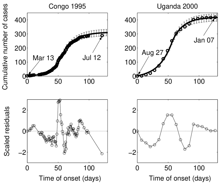
Figure 5: (Top) Comparison of the cumulative number of Ebola cases during the Congo 1995 and Uganda 2000 Ebola outbreaks, as a function of the time of onset of symptoms. Circles are the data. The solid line is the average of $250$ Monte Carlo replicates and the error bars represent the standard error around the mean from the simulation replicates using our parameter estimates (Table 1). For the case of Congo $1995$, simulations were begun on $13$ Mar $1995$. A reduction in the transmission rate $\beta$ due to the implementation of interventions occurs on $09$ May 1995 (day $56$) [12]. For the case of Uganda $2000$, simulations start on $27$ August $2000$ and interventions take place on $22$ October $2000$ (day $56$) [13]; (bottom) comparison of the residuals (difference between the data and the model best fit) scaled by the standard deviation for the cases of Congo and Uganda.

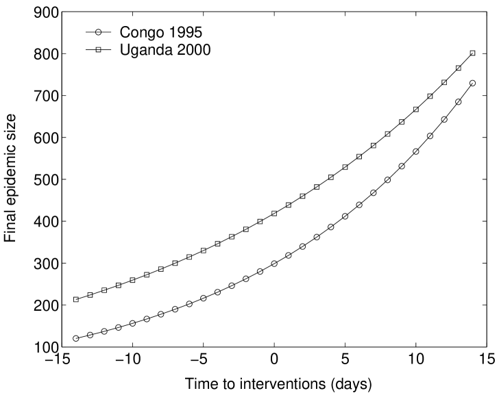
Figure 7: Sensitivity of the final epidemic size to the time of start of interventions. Here negative numbers represent number of days before the actual reported intervention date (Table 2) and positive numbers represent a delay after the actual reported intervention date ($\tau=0$). All other parameters have been fixed to their baseline values (Table 2). The final epidemic size grows exponentially as expected with the time of interventions with a rate of $0.06$ for the case of Congo and $0.05$ for the case of Uganda.

References

- [1] Centers for Disease Control (CDC). Ebola Hemorrhagic Fever. (http://www.cdc.gov/ncidod/dvrd/spb/mnpages/dispages/ebola.htm), accessed on August 24, 2003.
- [2] Centers for Disease Control (CDC). Ebola Hemorrhagic Fever: Table Showing Known Cases and Outbreaks, in Chronological Order. (http://www.cdc.gov/ncidod/dvrd/spb/mnpages/dispages/ebotabl.htm), accessed on August 24, 2003.
- [3] World Health Organization (WHO). Ebola Hemorrhagic Fever: Disease Outbreaks. (http://www.who.int/disease-outbreak-news/disease/A98.4.htm), accessed on October 17, 2003.
- [4] Breman, JG, Johnson, KM, van der Groen, G, et al. A search for for Ebola virus in animals in the Democratic Republic of the Congo and Cameroon: ecologic, virologic, and serologic surveys 1979-1980. J Inf Dis 1999;179:S139-47.
- [5] Leirs, H, Mills, JN, Krebs, JW, et al. Search for the Ebola Virus Reservoir in Kikwit, Democratic Republic of the Congo: Reflections on a Vertebrate Collection. J Inf Dis 1999;179:S155-63.
- [6] World Health Organization (WHO). Ebola Hemorrhagic Fever. (http://www.who.int/inf-fs/en/fact103.html), accessed on August 24, 2003.
- [7] Breman, JG, Piot, P, Johnson, KM, et al. The Epidemiology of Ebola Hemorrhagic Fever in Zaire, 1976. Proc Int Colloquium on Ebola Virus Inf held in Antwerp, Belgium, December 1977.
- [8] Birmingham, K and Cooney, S. Ebola: small, but real progress (news feature). Nature Med 2002;8:313.
- [9] Anderson, RM and May, RM. Infectious Diseases of Humans. Oxford University Press, Oxford, 1991.
- [10] Brauer, F, Castillo-Chavez, C. Mathematical Models in Population Biology and Epidemiology, Springer-Verlag, New York, 2000.
- [11] Renshaw, E. Modelling Biological Populations in Space and Time. Cambridge University Press, Cambridge, 1991.
- [12] Khan, AS, Tshioko, FK, Heymann, DL, et al. The Reemergence of Ebola Hemorrhagic Fever, Democratic Republic of the Congo, 1995. J Inf Dis 1999;179:S76-86.
- [13] World Health Organization (WHO). Outbreak of Ebola hemorrhagic fever, Uganda, August - January . Weekly epidemiological record 2001;76:41-48.
- [14] Piot, P, Bureau, P, Breman, G. D. Heymann, et al. Clinical Aspects of Ebola Virus Infection in Yambuku Area, Zaire, 1976. Proc. Int. Colloquium on Ebola Virus Inf. held in Antwerp, Belgium, December 1977.
- [15] Bickel, P, Doksum, KA. Mathematical Statistics. Holden-Day, Oakland, California, 1977.
- [16] The World Gazetteer. Democratic Republic of the Congo. (http://www.world-gazetteer.com/fr/fr_cd.htm), accessed on August , 2003.
- [17] UN-HABITAT (United Nations Human Settlelments Programme). Republic of Congo. website: (http://www.unhabitat.org/habrdd/conditions/midafrica/zaire.html), accessed on August 24, 2003.
- [18] Uganda Bureau of Statistics (UBOS). Website: (http://www.ubos.org/), accessed on August 24, 2003.
- [19] Castillo-Chavez, C, Velasco-Hernandez, JX and Fridman, S. Modeling Contact Structures in Biology. In: S.A. Levin ed., Frontiers of Theoretical Biology, Lecture Notes in Biomathematics 100, Springer-Veralg,Berlin-Heidelberg-New York 1994:454-91.
- [20] De Jong, MCM, Diekmann, O and Heesterbeek, H. How does transmission of infection depend on population size?. In: Mollison, D, ed. Epidemic models: Their structure and relation to data, Cambridge University Press, 1995:84-94.
- [21] Sartwell, PE. The distribution of incubation periods and the dynamics of infectious disease. Am J Epidem 1966;83:204-216.
- [22] Blower, SM, Dowlatabadi, H. Sensitivity and uncertainty analysis of complex models of disease transmission: an HIV model, as an example. Int Stat Rev 1994;2:229-243.
- [23] Niikura, M, Ikegami, T, Saijo, M, et al. Analysis of Linear B-Cell Epitopes of the Nucleoprotein of Ebola Virus That distinguish Ebola Virus Subtypes, Clin Diagn Lab Immunol 2003;10:83-87.
- [24] Chowell, G, Fenimore, PW, Castillo-Garsow, MA, et al. SARS Outbreaks in Ontario, Hong Kong and Singapore: the role of diagnosis and isolation as a control mechanism. J Theor Biol 2003;24:1-8.
- [25] Chowell, G, Castillo-Chavez, C, Fenimore, PW, et al. Implications of an Uncertainty and Sensitivity analysis for SARS’s Basic Reproductive Number for General Public Health Measures (submitted).
- [26] Nabel, GJ. Surviving Ebola virus infection (news feature). Nature 1999;4:373-374.
- [27] Sullivan, NJ, Geisbert, TW, Geibsert, JB, et al. Accelerated vaccination for Ebola virus haemorrhagic fever in non-human primates. Nature 2003;424:681-684.
- [28] Clarke T and Knight, J. Fast vaccine offers hope in battle with Ebola. Nature 2003;424:602.