Activity-dependent brain model explaining EEG spectra

Abstract

Most brain models focus on associative memory or calculation capability, experimentally inaccessible using physiological methods. Here we present a model explaining a basic feature of electroencephalograms (EEG). Our model is based on an electrical network with threshold firing and plasticity of synapses that reproduces very robustly the measured exponent 0.8 of the medical EEG spectra, a solid evidence for self-organized criticality. Our result are also valid on small-world lattices. We propose that an universal scaling behaviour characterizes many physiological signal spectra for brain controlled activities.

One of the most astonishing properties of the brain is its plasticity, i.e. the ability to modify the structural and functional properties of synapses, occurring mostly during development and learning alb . The mammalian central nervous system relies on precise synaptic circuits to function correctly. These circuits are assembled during development by the formation of synaptic connections between hundreds of thousands of neurons. Although molecular interactions direct the early formation of circuitry, this initial patterning is followed by a prolonged period during which the establishment of highly organized synaptic circuits in the developing human brain is thought to depend on neural activity. This transforms immature circuits into the organized connections that subserve adult brain function kat . In the central nervous system much of this plastic sculpting of neuronal connections is thought to occur during ”critical periods” of early postnatal life hen , when circuits are particularly susceptible to electrical activity triggered by external sensory inputs kat2 .

The most compelling and reliable models of activity-dependent synaptic plasticity in the brain are Long Term Potentiation (LTP) and Long Term Depression (LTD): persistent increases and decreases in synaptic efficacy that can be elicited in mammalian neurons, based on recent patterns of activity. LTP of synaptic transmission is traditionally elicited by synchronous, high-frequency inputs, whereas LTD typically occurs following repeated low frequency afferent stimulation pau . Strong evidence suggests that LTP and LTD are candidate mechanisms mediating activity-dependent synaptic plasticity during brain development kat , and many forms of adaptive behaviour, including learning and memory bra .

In the last years many different time series emerging from neural activities alb have been analysed through power spectra and generically power-law decay has been observed. This behaviour remains unexplained. Understanding its origin is not only a major theoretical challenge but also of eminent importance in many applications, in particular to give a solid basis to the interpretation of EEG gev ; buz . A large number of time series analyses have been performed on medical data that are directly or indirectly related to brain activity. Prominent examples are EEG data which are used by neurologists to discern sleep phases, diagnose epilepsy and other seizure disorders as well as brain damage and disease gev . An other example of a physiological function which can be monitored by time series analysis is the human gait which is controlled by the brain hau . For all these time series the power spectrum, i.e. the square of the amplitude of the Fourier transformation double logarithmically plotted against frequency, generally features a power law at least over one or two orders of magnitude with exponents between 1 and 0.7. On top of this background power law, additional structures give information on the details of the pathology and can point to specific resonance, frequency cut-offs and other deviations. While much focus is given to these secondary structures, the basic power law remains largely unexplained.

Models for brain activity based on the convolution of oscillators ash or stochastic waiting times iva have been proposed. They are essentially abstract representations on a mesoscopic scale, but none of them is based on the behaviour of a neural network itself. In order to get real insights on the relation between these time series and the microscopic, i.e. cellular, interactions inside a neural network, it is necessary to identify the essential ingredients of the brain activity responsible for characteristic scale-free behaviour observed through the power law of the spectrum, as discussed above. This insight is the basis for any further understanding of the diverse additional features that are observed and interpreted by practitioners that analyse these time series for diagnosis. Therefore the formulation of the right brain model that yields the correct power spectrum is of crucial importance for any further progress in the understanding of the living brain.

Here we report on a new model that captures the three most important ingredients yielding the expected power law, namely threshold firing, synapse adaption and network plasticity, including both LTP and LTD. Despite its simplicity our model reproduces with astonishing precision the experimentally observed exponent of the power spectrum, already for rather small networks. In agreement with real data, this exponent turns out to be extremely robust against modifications of the various parameters of the model. With this result we claim having made a breakthrough in the generic understanding of the diverse electrical time series.

We consider a simple square lattice of size $L\times L$ on which each site represents the cell body of a neuron, each bond a synapse. Therefore, on each site we have a potential $v_{i}$ and on each bond a conductance $g_{ij}$. Whenever at time $t$ the value of the potential at a site $i$ is above a certain threshold $v_{i}\geq v_{\rm max}$, approximately equal to $-55mV$ for the real brain, the neuron fires, i.e. generates an ”action potential”, distributing charges to its connected neighbours in proportion to the current flowing through each bond

$$v_{j}(t+1)=v_{j}(t)+v_{i}(t){i_{ij}(t)\over\sum_{k}i_{ik}(t)}$$

where $v_{j}(t)$ is the potential at time $t$ of site $j$, nearest neighbor of site $i$, $i_{ij}=g_{ij}(v_{i}-v_{j})$ and the sum is extended to all nearest neighbors $k$ of site $i$ that are at a potential $v_{k}<v_{i}$. The conductances are initially all set equal to unity whereas the neuron potentials are uniformly distributed random numbers between $v_{\rm max}-2$ and $v_{\rm max}-1$. The potential is fixed to zero at top and bottom whereas periodic boundaries are imposed in the other direction.

The system is stimulated at one input (source), a site in the centre of the lattice, and the electrical activity is monitored as function of time by measuring the total current flowing in the system. The firing rate of real neurons is limited by the refractory period, i.e. the brief period after the generation of an action potential during which a second action potential is difficult or impossible to elicit. The practical implication of refractory periods is that the action potential does not propagate back toward the initiation point and therefore is not allowed to reverberate between the cell body and the synapse. In our model, once a neuron fires, it remains quiescent for one time step and it is therefore unable to accept charge from firing neighbours. This ingredient indeed turns out to be crucial for a controlled functioning of our numerical model. In this way an avalanche of charges can propagate far from the input through the system similarly to the dynamics of self-organized critical systems bak , as observed in organotypic cultures from coronal slices of rat cortex beg where neuronal avalanches are stable for many hours beg2 .

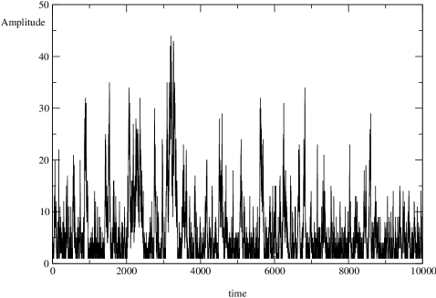
Figure 1: Total current flowing in one configuration of lattice ($L=1000$) as function of time in a sequence of several thousand stimuli. The value of the parameters is $\alpha=0.03$, $\sigma_{t}=0.0001$, $v_{\rm max}=6$.

Every site that at a given time $t$ is at or above threshold $v_{\rm max}$ fires according to eq. (1), then the conductance of all the bonds that have carried a current is increased in the following way

$$g_{ij}(t+1)=g_{ij}(t)+\delta g_{ij}(t)$$

where $\delta g_{ij}(t)=k\alpha i_{ij}(t)$, with $\alpha$ being a dimensionless parameter and $k$ a unit constant bearing the dimension of an inverse potential. After applying eq. (2) the time variable of our simulation is increased by one unit. Eq. (2) describes the LTP mechanism, whose strength is tuned by the parameter $\alpha$. Once an avalanche of firings comes to an end, the conductance of all the bonds with non-zero conductance is reduced by the average conductance increase per bond,

$$\Delta g=\sum_{ij,t}\delta g_{ij}(t)/N_{b}$$

where $N_{b}$ is the number of bonds with non-zero conductance. Eq. (3) implements the LTD process. The quantity $\Delta g$ depends on $\alpha$ and on the response of the brain to a given stimulus. In this way our electrical network ”memorizes” the most used paths of discharge by increasing their conductance, whereas the less used synapses atrophy. Once the conductance of a bond is below an assigned small value $\sigma_{t}$, we remove it, i.e. set it equal to zero, which corresponds to what is known as pruning. This remodelling of synapses mimicks the fine tuning of wiring that occurs in the developing brain, when neuronal activity can modify the synaptic circuitry, once the basic patterns of brain wiring are established alb .

Our brain is driven by setting the potential of the input site to the value $v_{\rm max}$, corresponding to one stimulus. We let the discharge evolve until no further firing occurs, then we apply the next stimulus. Fig.1 shows the electrical signal as function of time: the total current flowing in the system is recorded in time during a sequence of successive avalanches. As defined above the time unit corresponds to the time necessary to propagate the signal from a neuron to next nearest neighbours. Data show that discharges of all sizes are present in the brain response, reminiscent of self-organized criticality where the avalanche size distribution scales as a power law beg .

Figure 2: The number of pruned bonds as function of time in a lattice of linear size $L=100$ for different values of $\alpha$. The value of the parameters is $\sigma_{t}=0.0001$ and $v_{\rm max}=6$.

The pruning mechanism introduced in the model depends on the strength of the parameter $\alpha$, that controls both the LTP and LTD processes. In fact, the more the system learns strengthening the used synapses, the more the unused connections will weaken. Fig. 2 shows the number of pruned bonds in the system as function of time for different values of $\alpha$: For large values of the parameter ( e.g. $\alpha=0.08$) the system strengthens more intensively the synapses carrying current but also very rapidly prunes the less used connections, reaching after a short transient a plateau where it prunes very few bonds. On the contrary, for small values of $\alpha$ (equal to 0.005) the system takes more time to initiate the pruning process and slowly reaches a plateau. The number of active (non-pruned) bonds asymptotically reaches its largest value at the value $\alpha=0.03$. This could be interpreted as an optimal value for the system with respect to the joint mechanisms LTP-LTD. Indeed LTD seems to be the necessary counterpart to LTP in order to modulate the synaptic strength ros . The asymptotic plateau value for varying $\alpha$ is found within the extreme values shown in Fig.2.

After $N_{p}$ stimuli the network is no longer a simple square lattice due to pruning, and constitutes the first approximation to a trained brain, on which we are going to perform our measurements. These consist of a new sequence of stimuli at the input site, each one of them again triggered by the voltage set at threshold, during which we measure the number of firing neurons as function of time. This quantity corresponds to the total current flowing in a discharge measured by the electromagnetic signal of the EEG. In order to compare with medical data, we calculate the power spectrum of the resulting time series, i.e. the square of the amplitude of the Fourier transform as function of frequency.

In Fig. 3 we show the power spectrum obtained with our model in a log-log-plot with the parameters $\alpha=0.03$, $N_{p}=10$, $\sigma_{t}=0.0001$, $v_{\rm max}=6$ and a lattice of size $L=1000$ and see that it yields a power law with the exponent $0.8\pm 0.1$. This is exactly the same value for the exponent found generically on medical EEG power spectra fre ; nov . We also show in Fig. 3 the EEG obtained from channel 17 in the left hemisphere of a male subject, as measured in ref.nov having the exponent 0.795.

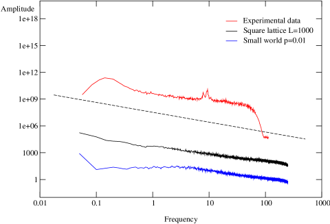
Figure 3: Power spectra for experimental data and numerical data ($L=1000$, $\alpha=0.3$, $N_{p}=10$, $v_{\rm max}=6$) for the square lattice (middle curve) and the small world lattice (bottom curve, $L=1000$, $\alpha=0.05$, $N_{p}=1000$, $v_{\rm max}=8$) with $1\%$ rewired bonds. The experimental data (top curve) are from ref. (16). The numerical data are averaged over 10 different network configurations. The dashed line has a slope 0.8.

The exponent 0.8 that we observed in the power spectrum of our ”brain” is stable against changes of the parameters $\alpha$, $v_{\rm max}$, $\sigma_{t}$, and $N_{p}$, and it is also found in the case of random initial conductance on the bonds of the lattice. We also simulate the brain dynamics on a square lattice with a small fraction of bonds, from 0 to $10\%$, rewired to long range connections corresponding to a small world network wat ; lag ; she , which more realistically reproduces the connections in the real brain. Fig.3 shows the power spectrum for a system with $1\%$ rewired bonds and a different set of parameters $\alpha$, $N_{p}$, $v_{\rm max}$: the spectrum has some deviations from the power law at small frequencies and tends to the same universal scaling behaviour at larger frequencies over two orders of magnitude. The same behaviour is found for a larger fraction of rewired bonds, up to $30\%$.

Although we cannot justify the exponent 0.8 beyond the numerical result of our model, it seems clear that this value corresponds to a universal number characterizing a larger class of brain networks including real brains. Medical studies of EEG focus on subtle details of a power spectrum (e.g. shift in peaks) to discern between various pathologies. These detailed structures however live on a background power law spectrum that shows universally an exponent of about 0.8, as measured for instance in refs. fre and nov . A similar exponent was also detected in the spectral analysis of the stride-to-stride fluctuations in the normal human gait which can directly be related to neurological activity hau . We have been able to reproduce this universal exponent with a simple electrical toppling model that includes pruning. This success is very encouraging since it can provide insight to understand its origin and open new perspectives to model pathological features of EEG spectra by including more realistic details into our model.

Acknowledgements. We gratefully thank E. Novikov and collaborators for allowing us to use their experimental data. We also thank Salvatore Striano, MD, for discussions and Stefan Nielsen and Hansjörg Seybold for help.

References

- (1) T. D. Albraight, T. M. Jessel, E. R. Kandel, M. I. Posner, Neuron, Review supplement to vol.59 (February 2000).
- (2) L. C. Katz, C. J. Shatz, Science 274, 1133 (1996).
- (3) T. K. Hensch, Ann. Rev. Neurosci. 27, 549 (2004).
- (4) L.C. Katz, J.C. Crowley, Nat. Rev. Neurosci. 3, 34 (2002).
- (5) O. Paulsen, T. J. Sejnowski, Curr. Opin. Neurobiol. 10, 172 (2000).
- (6) K. H. Braunewell, D.Manahan-Vaughan, Rev. Neurosci. 12, 121 (2001).
- (7) A. Gevins, H. Leong, M. E. Smith, J. Le , R. Du, Trends Neurosci. 18, 429 (1995).
- (8) G. Buzsaki, A. Draguhn, Science 304, 1926 (2004).
- (9) J. M. Hausdorff et al., Physica A. 302, 138 (2001).
- (10) Y. Ashkenazy, J. M. Hausdorff, P. C. Ivanov, E. H. Stanley, Physica A. 316, 662 (2002).
- (11) P. Ch. Ivanov, L. A. N. Amaral, A. L. Goldberger, H. E. Stanley, Europhys. Letters 43, 363 (1998).
- (12) P. Bak, How nature works. The science of self-organized criticality (Springer, New York, 1996).
- (13) J. M. Beggs, D. Plenz, J. Neurosci. 23, 11167 (2003).
- (14) J. M. Beggs, D. Plenz, J. Neurosci. 24, 5216 (2004).
- (15) E.S. Rosenzweig, C.A. Barnes, B.L. McNaughton, Nat. Neurosci. 5, 48 (2002).
- (16) W. J. Freeman, L. J. Rogers, M. D Holmes., D. L. Silbergeld, J. Neurosci. Meth. 95, 111 (2000).
- (17) E. Novikov, A. Novikov, D. Shannahoff-Khalsa, B. Schwartz, J. Wright, Physical Review E. 56, 3 (1997).
- (18) D. J. Watts, S. H. Strogatz, Nature 393, 440 (1998).
- (19) L. F. Lago-Fernandez, R. Huerta, F. Gorbacho , J. A. Siguenza, Phys. Rev. Lett. 84, 2758 (2000).
- (20) O. Shefi, I. Golding, R. Seger, E. Ben-Jacob, A. Ayali, Physical Review E. 66, 021905 (2002).