Action Potential Onset Dynamics and the Response Speed of Neuronal Populations

Abstract

The result of computational operations performed at the single cell level are coded into sequences of action potentials (APs). In the cerebral cortex, due to its columnar organization, large number of neurons are involved in any individual processing task. It is therefore important to understand how the properties of coding at the level of neuronal populations are determined by the dynamics of single neuron AP generation. Here we analyze how the AP generating mechanism determines the speed with which an ensemble of neurons can represent transient stochastic input signals. We analyze a generalization of the $\theta$-neuron, the normal form of the dynamics of Type-I excitable membranes. Using a novel sparse matrix representation of the Fokker-Planck equation, which describes the ensemble dynamics, we calculate the transmission functions for small modulations of the mean current and noise noise amplitude. In the high-frequency limit the transmission function decays as $\omega^{-\gamma}$, where $\gamma$ surprisingly depends on the phase $\theta_{s}$ at which APs are emitted. If at $\theta_{s}$ the dynamics is insensitive to external inputs, the transmission function decays as (i) $\omega^{-3}$ for the case of a modulation of a white noise input and as (ii) $\omega^{-2}$ for a modulation of the mean input current in the presence of a correlated and uncorrelated noise as well as (iii) in the case of a modulated amplitude of a correlated noise input. If the insensitivity condition is lifted, the transmission function always decays as $\omega^{-1}$, as in conductance based neuron models. In a physiologically plausible regime up to $1\textrm{kHz}$ the typical response speed is, however, independent of the high-frequency limit and is set by the rapidness of the AP onset, as revealed by the full transmission function. In this regime modulations of the noise amplitude can be transmitted faithfully up to much higher frequencies than modulations in the mean input current. We finally show that the linear response approach used is valid for a large regime of stimulus amplitudes.

I Introduction

Neurons are the basic building blocks of neural networks and thus constitute the computational units of the brain. They dynamically transform synaptic inputs into output action potential (AP) sequences. To conceive the complex computational capabilities of the brain, it is crucial to understand this transformation and to identify simple neuron models which accurately reproduce the dynamical features of cortical neurons.

Here we study this mapping in a reduced neuron model. This model is obtained by a generalization of the $\theta$-neuron Ermentrout84 ; Gutkin98 , which is a canonical phase oscillator model of excitable neuronal membranes exhibiting Type-I excitability. Phase oscillator models have a long history in physics and biology Coddington55 ; Winfree74 ; Guckenheimer75 ; Winfree01 and recently they were introduced in theoretical neuroscience Ermentrout84 . In contrast to integrate-and-fire models, which are phenomenological models of cortical neurons, they can be derived from the limit cycle dynamics of conductance based neuron models, reducing the complex dynamics which usually incorporates many degrees of freedom to a single phase variable. This reduction is an important prerequisite for analytical studies of either the dynamics of single neurons or of neural networks.

Cortical neurons in vivo are subject to an immense synaptic bombardment, resulting in large fluctuations of their membrane potential (MP) Destexhe99 ; Volgushev00 ; Anderson00 and irregular action potential firing Softky93 . Because the exact computational role of these fluctuations is largely unknown, it was suggested to treat them as a random process, dividing the synaptic input into a mean input current and a random fluctuating contribution Tuckwell88 with a given correlation time $\tau_{c}$. The fluctuations can serve as a potentially independent information channel because when the afferent activity of a neuron changes, not only the mean input is affected, but also the amplitude of the fluctuationsVreeswijk96 ; Brunel99 ; Lindner02 .

The stationary response properties of the classical $\theta$-neuron subject to fluctuating input currents were calculated in Gutkin98 ; Lindner03 for a temporally uncorrelated input and in Brunel03 for a temporally correlated input current. Both studies showed that the $\theta$-neuron can reproduce the stationary response properties exhibited by many cortical neurons, i.e. a square-root dependence of the firing rate on the input current close to threshold for small noise amplitudes Tateno04 and irregular firing in the noise driven regime. Despite its success to reproduce the stationary firing behavior of cortical neurons, the $\theta$-neuron lacks a crucial dynamical feature: The fast action potential upstroke exhibited by conductance based neuron models. Here we study a generalization of the classical $\theta$-neuron with an adjustable action potential onset speed, introducing a phenomenological term which mimics the fast activation of sodium channels.

We derive the time dependent response in the presence of temporally correlated noise to a modulation in the mean input current and a modulation in the noise amplitude. For both modulation paradigms we calculate the high frequency limit. In this limit, the response amplitude decays as $\omega^{-\gamma}$, where the integer exponent $\gamma$ is completely independent of the action potential onset dynamics and surprisingly only depends on the oscillator phase $\theta_{s}$, at which an action potential is emitted: If at $\theta_{s}$ the dynamics is insensitive to external inputs, the transmission function decays as (i) $\omega^{-3}$ for the case of a modulation of an uncorrelated noise amplitude and as (ii) $\omega^{-2}$ for a modulation of the mean input current in the presence of a correlated and uncorrelated noise as well as (iii) in the case of a modulated amplitude of a correlated noise input. If the insensitivity condition is lifted, the transmission function always decays as $\omega^{-1}$, as in conductance based neuron models.

The full transmission function is then calculated via the eigenvalues and eigenfunctions of the Fokker-Planck operator, which describes the dynamics of the ensemble averaged probability density function. The eigenvalues and eigenfunctions are computed using a high performance iterative scheme, the Arnoldi method Trefethen97 ; Lehoucq98 , from a novel sparse matrix representation of the Fokker-Planck operator. This method allows for a fast computation and high numerical precision, hard to achieve by direct numerical simulations.

We then demonstrate that the response amplitudes for the classical $\theta$-neuron typically exhibit a cut-off behavior, where the cut-off frequency, which is closely linked to the spectral properties of the Fokker-Planck operator, is approximately given by the neurons stationary firing rate. Stimulations at frequencies larger than the cut-off frequency are strongly damped. For an increasing action potential onset speed at a fixed stationary rate, stimuli with much larger frequencies can be transmitted almost unattenuated. We show that the response amplitude for the case of a noise modulation typically decays much slower than in the case of a mean input current modulation.

The impact of noise on the dynamic response properties was previously almost exclusively studied in integrate-and-fire models Lapicque07 ; Tuckwell88 . The first studies were pioneered by Knight Knight72 , who considered a simple integrator model, in which the firing threshold is drawn randomly, every time an action potential occurs. These results were then extended to models, where the reset voltage was also drawn randomly, and to models in which the the input changed either very slowly, or to spike response models, where the input is assumed to change very fast Gerstner00 . Recently, the impact of current noise on the dynamical response of the leaky integrate-and-fire model was investigated Brunel99 ; Brunel00 ; Brunel01 ; Fourcaud02 ; Lindner02 . In these studies it was shown that integrate-and-fire models driven by a synaptic fluctuating input exhibit a linear response amplitude which does not decay to zero in the high frequency limit. This lead some to the conclusion that cortical neurons can transmit information instantaneously Brunel01 ; Lindner02 . Only recently, this interpretation was questioned by two studies Naundorf03 ; Fourcaud03 which demonstrated that the unattenuated transmission of high frequency signals in integrate-and-fire models are more a consequence of the oversimplification of the model rather than property of real neurons.

II Material and Methods

II.1 Model

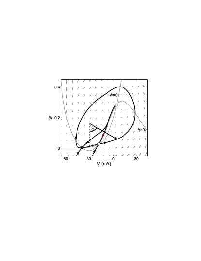
Figure 1: Phase plane of a type-I single compartment conductance based model (Morris-Lecar model Morris81 ) in the excitable regime (filled dot: stable fixed point, open dots: unstable fixed points). Gray lines are the nullclines, denoted by $\dot{w}=0$ and $\dot{V}=0$. Black lines are stable and unstable manifolds of the saddle and the node. The excitable dynamics can be reduced to a phase oscillator with one degree of freedom parameterized by the angle $\vartheta$.

The model is based on the normal form of the dynamics of type-I membranes at the bifurcation to repetitive firing. Conductance based neuron models which exhibit Type-I excitability typically undergo a saddle-node bifurcation of codimension one, when brought to repetitive firing. A center-manifold reduction at the bifurcation point leads to the following normal form Strogatz95 :

$$C\dot{\bar{V}}=\frac{g}{V_{0}}\left(\bar{V}-V^{*}\right)^{2}+\left(\bar{I}(t)-I_{c}\right),$$ (1)

which is a dynamical equation for the MP $\bar{V}$ of the neuron. The input current relative to the rheobase $I_{c}$ of the neuron is denoted by $\bar{I}(t)$. The constants $A$ and $V^{*}$ can be deduced from a given multidimensional conductance based model. It is convenient to introduce dimensionless quantities $V$and $I$:

$$V = \left(\bar{V}-V^{*}\right)/V_{0}$$ (2)

$$I(t) = \left(\bar{I}(t)-I_{c}\right)/\left(gV_{0}\right)$$ (3)

and the effective time constant:

$$\tau=C/g$$ (4)

The rescaled dynamics is then given by:

$$\tau\dot{V}=V^{2}+I(t)$$ (5)

For $I(t)>0$, the MP has a finite “blow-up” time, meaning that it needs a finite time to get from $-\infty$ to $+\infty$, where both ends of the real axis are identified, turning the model into a phase oscillator. The normal form Eq. (5) is equivalent to a phase oscillator, the $\theta$-neuron Ermentrout84 ; Gutkin98 . Its equation of motion,

$$\tau\dot{\theta}=\left(1-\cos\theta\right)+I(t)\left(1+\cos\theta\right)$$ (6)

is found by substituting $V=\tan\left(\theta/2\right)$ with the angle variable $\theta$ in the interval $(-\pi,\pi]$.

In the model, a spike is emitted each time $\theta$ reaches the value $\theta_{s}$. By choosing $\theta_{s}=\pi$, the original $\theta$-neuron is obtained. Figure 1 illustrates schematically the reduction of a conductance based neuron model to a phase oscillator model.

Although the $\theta$-neuron is the normal form of the dynamics at the bifurcation, it lacks the rapid AP onset exhibited by conductance based neuron models and real neurons. To account for this dynamical feature we generalized the model to reflect the rapid depolarization of the membrane resulting from the fast kinetics of sodium conductances in the following way:

$$\tau\dot{V}=V^{2}+I(t)+\alpha\left(1+\tanh(\beta V)\right),$$ (7)

where we introduced two additional parameters $\alpha$ and $\beta$. The sigmoidal term phenomenologically models the part of the sodium channel activation curve, which is not included in the $V^{2}$-term of the normal form. The parameter $\alpha$ controls the sodium peak conductance and the parameter $\beta$ the width of this activation curve. Both parameters control the rapidness of the AP onset. As for the normal form an equivalent phase oscillator equation can be found by substituting $V=\tan\left(\theta/2\right)$:

$$\tau\dot{\theta} = \left(1-\cos\theta\right)+\left(1+\cos\theta\right)\cdot$$

$$+\left\{I(t)+\alpha\left(1+\tanh(\beta\tan\left(\theta/2\right)\right)\right\}$$

II.2 Fluctuating input currents

In vivo, neurons are subject to an ongoing synaptic bombardment, resulting in a fluctuating MP. To model this situation, we assume a temporally fluctuating input current,

$$I(t)=I_{0}+\sigma z(t),$$ (9)

composed of a mean $I_{0}$ and a stationary fluctuating part $\sigma z(t)$, where $z(t)$ is an Ornstein-Uhlenbeck process with a given correlation function $\left\langle z(t)z(t^{\prime})\right\rangle=\exp\left(-t/\tau_{c}\right)$. Thus $z(t)$ obeys the Langevin equation Gardiner85 ,

$$\tau_{c}\frac{d}{dt}z(t)=-z+\sqrt{\tau}\eta(t)$$ (10)

with $\left\langle\eta(t)\right\rangle=0$ and $\left\langle\eta(t)\eta(t^{\prime})\right\rangle=\delta(t-t^{\prime})$. Eq. (6) and Eq. (II.1) describe a realization of the dynamics of a single neuron. Since the input is fluctuating and we are interested in coding at population level it is natural to consider an ensemble of such units, described by the time dependent probability density function $P(\theta,z,t)$. Its dynamics is determined by the Fokker-Planck equation Risken96 :

$$\partial_{t}P(\theta,z,t)=\hat{L}P(\theta,z,t),$$ (11)

with,

$$\hat{L} = -\tau^{-1}\partial_{\theta}\left\{\left(1-\cos\theta\right)\right.$$ (12)

$$+\left(I_{0}+\sigma z+\alpha\left(1+\tanh\left(\beta\tan\left(\theta/2\right)\right)\right)\right)$$

$$\left.\vphantom{\left(I_{0}\right)}\cdot\left(1+\cos\theta\right)\right\}+\tau_{c}^{-1}\partial_{z}\left(z+\frac{\tau}{2\tau_{c}}\partial_{z}\right).$$

The boundary conditions for $P(\theta,z,t)$ are periodic in the $\theta$- and natural in the $z$-direction.

II.3 Time dependent firing rate

The ensemble averaged firing rate is given by the probability current across the line $\theta=\theta_{s}$ with positive velocity. At $\theta_{s}=\pi$ the dynamics is independent of the input current $I(t)$ and the rate is equal to the probability current through the entire line $\theta=\pi$:

$$\nu(t)=2\int_{-\infty}^{\infty}dz\,P(\pi,z,t)$$ (13)

Although quite convenient for analytical considerations, the definition of this spike-phase is, however, rather arbitrary. In the normal form, the point $\theta_{s}=\pi$ corresponds to the point $V=\infty$, where the model reflects least the dynamics at the bifurcation. To assess if this particular choice has any influence on the dynamical response properties of the model, we also calculate the firing rate at $\theta_{s}=\pi-\delta$. The probability current through this line is given by:

$$J_{\theta} = \tau^{-1}\int_{-\infty}^{\infty}P(\theta_{s},z,t)\left((1-\cos\theta_{s})\right.$$

$$\!\!\!\left.+(I_{0}+\sigma z+\alpha(1+\tanh(\beta\tan(\theta_{s}/2)))\right)\,dz$$

The rate is, however, not exactly given by the flux $J_{\theta}$. There is a contribution from trajectories, which are driven back below the threshold due to the external fluctuations. For a correlated input current, however, the introduced error is exponentially small. This can be seen in Eq. (II.1). For small values of $\delta$, the probability distribution $P(\theta,\dot{\theta})$ around $\pi-\delta$ is a Gaussian with a mean value $2-\delta^{2}$ and a width $\propto\delta^{2}$. The negative part of this Gaussian is proportional to:

$$\left(2\pi\delta^{4}\sigma^{2}\right)^{-1/2}\int_{-\infty}^{0}\exp\left(-\frac{\left(x-(2-\delta^{2})\right)^{2}}{2\delta^{4}\sigma^{2}}\right)\,dx$$ (15)

For all practical purposes ($\delta<0.5$ and $\sigma<1$), this integral is smaller than $10^{-10}$. We will see, however, that the definition $\theta_{s}=\pi$ in the classical $\theta$-neuron qualitatively changes the dynamic response of the model in the high frequency limit.

II.4 Parameter choice

Before discussing the stationary and dynamical properties of the generalized $\theta$-neuron we would like to define a biologically plausible parameter regime. The parameters which we need to fix are the time constant $\tau$, the mean input current $I_{0}$, the strength of the fluctuating input $\sigma$ and the synaptic input correlation time $\tau_{c}$. An estimate of the correlation time of the MP is given by approximating the dynamics for $I_{0}<0$ near the stable fixed point by an Ornstein-Uhlenbeck process. Straightforward linearization around the stable fixed point at $-\sqrt{I_{0}}$ then yields:

$$\tau_{\mathrm{relax}}\approx\tau\left(2\sqrt{I_{0}}\right)^{-1}$$ (16)

In the subthreshold noise-driven regime, which we will discuss in the following, we choose $I_{0}=-0.1$. The time constant $\tau$ is then adapted via Eq. (16), to achieve a relaxation time of approximately $5\textrm{ms}$, which leads to values for $\tau$ of approximately $3\textrm{ms}$.

The parameters $\alpha$ and $\beta$ parameterize the sodium activation curve, which, in conductance based models, determines the speed at the action potential onset. For the following numerical treatment we keep $\beta$, which mediates the width of the activation curve and is an intrinsic physiological parameter, fixed to a value of 20. The parameter $\alpha$, which represents the sodium peak conductance, is changed in the range from $0$ to $1$.

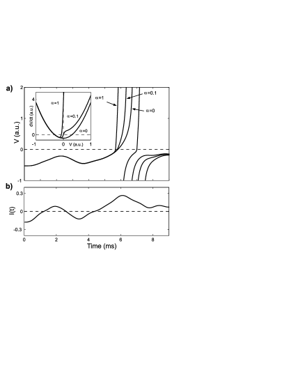
Figure 2: Increasing $\alpha$ leads to a sharper action potential onset. (a) Sample MP trajectories for $\alpha=0$, $\alpha=0.1$ and $\alpha=1$. The inset shows the deterministic part of Eq. (7). (b) Fluctuating input current $I(t)$. Parameters: $\tau_{c}=1.5\textrm{ms}$, $\sigma=0.3$, $I_{0}=-0.1$ and $\beta=20$. Right before AP onsets the trajectories are virtually identical.

Figure 2 shows three sample realizations of Eqs. (II.1, 9) for different values of the parameter $\alpha$. If the input current is positive for a sufficient amount of time, action potentials are initiated. With increasing values of $\alpha$ the sharpness at the onset increases, while the subthreshold fluctuations are not affected.

II.5 Dynamic Response Theory

Figure 3: Sketch of the population response paradigm. An ensemble of neurons receives a modulated noisy input current or a current, where the noise amplitude is modulated. The noise realization which each neuron receives is different, leading to different MP traces and AP sequences. The output quantity is the population averaged firing rate in the interval $[t,t+dt)$, $\nu(t)$.

For time-dependent input currents $\varepsilon I(t)$, the Fokker-Planck operator $\hat{L}(\theta,z,t)$ can always be split into two parts:

$$\hat{L}(\theta,z,t)=\hat{L}_{0}(\theta,z)+\varepsilon\hat{L}_{1}(\theta,z,t),$$ (17)

where $\hat{L}_{0}(\theta,z)$ is the time-independent part and $\hat{L}_{1}(\theta,z,t)$ contains all time-dependencies of the external input. In the following we require that the time-dependent inputs are small in magnitude, i.e. $\varepsilon\ll 1$. We then expand the general time-dependent solution in powers of $\varepsilon:$

$$P_{\mathrm{TD}}(\theta,z,t)=P_{0}(\theta,z)+\varepsilon\tilde{P}(\theta,z,t)+\mathcal{O}(\varepsilon^{2})$$ (18)

Inserting this solution into the Fokker-Planck equation and keeping only terms up to linear order in $\varepsilon$ leads to a dynamical equation for the time dependent part of the density $\tilde{P}(\theta,z,t)$:

$$\partial_{t}\tilde{P}(\theta,z,t)=\hat{L}_{0}(\theta,z)\tilde{P}(\theta,z,t)+\hat{L}_{1}(\theta,z,t)P_{0}(\theta,z)$$ (19)

Formally the solution of this equation is given by:

$$\tilde{P}(\theta,z,t)=\int_{-\infty}^{t}e^{\hat{L}_{0}(t-t^{\prime})}\hat{L}_{1}(\theta,z,t)P_{0}(\theta,z)\,dt^{\prime}$$ (20)

In the following we will consider stimuli of the type:

$$\hat{L}_{1}(\theta,z,t)=e^{i\omega t}\hat{L}_{1}(\theta,z)$$ (21)

Eq. (20) can then be readily solved, yielding:

$$\tilde{P}(\theta,z,t)=\sum_{k}\frac{c_{k}}{i\omega-\lambda_{k}}P_{k}(\theta,z)e^{i\omega t}$$ (22)

The $c_{k}$ are the expansion coefficients of $\hat{L}_{1}(\theta,z)P_{0}(\theta,z)$ into the eigenfunctions $P_{k}(\theta,z)$ of $\hat{L}_{0}(\theta,z)$. The time-dependent firing rate is given by Eq. (13):

$$\nu(t) = \tau^{-1}\int_{-\infty}^{\infty}dz\,\left((1-\cos\theta_{s})\right.$$ (23)

$$\left.+\left(I_{0}+\sigma z+\alpha(1+\tanh(\beta\tan(\theta_{s}/2)))\right)\right)$$

$$\cdot\left(P_{0}(\theta_{s},z)+\varepsilon\tilde{P}(\theta_{s},z,t)\right)$$

$$=: \nu_{0}+\varepsilon\nu_{1}(\omega)e^{i(\omega t+\varphi(\omega))}$$

In the following we will consider two types of external stimulations:

1. Modulations in the mean input current:

   $$I_{0}\longrightarrow I_{0}+\varepsilon e^{i\omega t}$$

2. Modulations in the noise amplitude:

   $$\sigma\longrightarrow\sigma+\varepsilon e^{i\omega t}$$

II.6 High frequency limit

In this section we sketch how to analytically calculate the asymptotic decay of $\nu_{1}(\omega)$ in the limit $\omega\to\infty$. Inserting Eq. (22) into Eq. (19) leads to:

$$\left(i\omega-\hat{L}_{0}\right)\tilde{P}(\theta,z,t)e^{-i\omega t}=\hat{L}_{1}P_{0}(\theta,z)$$ (24)

If the right hand side vanishes at $\theta=\theta_{s}$, $\tilde{P}(\theta,z,t)$ has to decay at least as $\omega^{-2}$. Differentiation of Eq. (19) with respect to $t$ and subsequent reinsertion leads to:

$$\left(\omega^{2}+\hat{L}_{0}\right)\tilde{P}(\theta,z,t)=-\hat{L}_{0}\hat{L}_{1}P_{0}(\theta,z)$$ (25)

If now the right hand side vanishes at $\theta=\theta_{s}$, Eq. (19) has to be differentiated again, until, after reinsertion, the right hand side is different from zero.

II.7 Matrix Method

As demonstrated the dynamical response properties of the generalized $\theta$-neuron to small time-dependent inputs are completely determined by the spectrum and eigenfunctions of the Fokker-Planck operator $\hat{L}$. To compute the dynamical response properties in the presence of a temporally correlated noise current for arbitrary stimulation frequencies we expand $\hat{L}$ into a complete orthonormal basis leading to a sparse matrix representation for which we compute the eigenvalues and eigenfunctions numerically. This approach has the advantage that the response properties can be computed with very high accuracy. The two subtleties we will have to deal with are that (1) the resulting matrix is very large in the parameter regime we are interested in (up to $10^{6}\times 10^{6}$) and (2) the operator $\hat{L}$ is not Hermitian and thus standard diagonalization procedures such as the Lanczos algorithm can not be applied. We solved both problems by using a basis-set, which results in a very sparse matrix representation, and by using a high performance iterative scheme, the Arnoldi method Lehoucq98 , to compute the eigenfunctions and the spectrum of this matrix to a high numerical accuracy.

II.8 Eigenvalues and eigenfunctions for a correlated noise input

II.8.1 Matrix equation

We first replace the probability density $P(\theta,z,t)$ in an eigenmode Ansatz with $e^{\lambda_{k}t}P_{k}(\theta,z)$. Inserting this into Eq. (11) the exponential cancels:

$$\lambda_{k}P_{k}(\theta,z)=\hat{L}P_{k}(\theta,z)$$ (26)

Due to the imposed boundary conditions, the set $\left\{\lambda_{k}\right\}$, i.e. the spectrum of $\hat{L}(\theta,z)$ is discrete. There is, however, a macroscopic drift in the system, meaning that detailed balance is not fulfilled and thus $\hat{L}$ is not Hermitian Gardiner85 . This means that the resulting spectrum $\left\{\lambda_{k}\right\}$ and the corresponding eigenfunctions $P_{k}(\theta,z)$ are complex. By complex conjugation of Eq. (26) it is easy to show that to every eigenvalue $\lambda_{k}$ with the corresponding eigenfunction $P_{k}(\theta,z)$, an eigenvalue $\lambda_{k}^{*}$ with the eigenfunction $P_{k}^{*}(\theta,z)$ exists. This guarantees that a real solution can always be constructed. The solution with $\lambda_{0}=0$ corresponds to the stationary density and the time dependent solution can always be given in terms of eigenfunctions and eigenvalues Risken96 :

$$P(\theta,z,t) = e^{\hat{L}(t-t_{0})}P_{\mathrm{initial}}(\theta,z)$$ (27)

$$= \sum_{k}a_{k}e^{\lambda_{k}(t-t_{0})}P_{k}(\theta,z)$$

with $P_{\mathrm{initial}}(\theta,z)=\sum_{k}a_{k}P_{k}(\theta,z)$. Although the eigenfunctions of $\hat{L}$ form a basis, it is important to note that they are not orthogonal. An important property is that the mean value of all eigenfunctions except $P_{0}(\theta,z)$ is zero:

$$\int_{-\pi}^{\pi}d\theta\int_{-\infty}^{\infty}dz\,P_{k}(\theta,z)=0$$ (28)

To actually compute the spectrum and eigenfunctions we expand $P(\theta,z)$ into a set of complete orthonormal functions:

$$P(\theta,z)=\sum_{m=0}^{\infty}a_{n,m}\psi_{n,m}(\theta,z)$$ (29)

with

$$\psi_{n,m}(\theta,z) = \left(2^{m+1}\sqrt{\pi\tau/2\tau_{c}}m!\right)^{-1/2}$$ (30)

$$e^{in\theta}H_{m}\left(\sqrt{2\tau_{c}/\tau}z\right)e^{-z^{2}\tau_{c}/\tau}.$$

This expansion obeys the imposed boundary conditions. In the $\theta$-directions it consists of plane waves, while in the $z$-direction harmonic-oscillator functions are used Gardiner85 with the Hermite polynomials $H_{m}(z)$ Abramowitz72 . We now insert Eq. (29) in Eq. (11). Multiplying from left with $\psi_{n^{\prime},m^{\prime}}^{*}(\theta,z)$ and integrating over the whole domain leads to a matrix eigenvalue equation for the $\left(a_{n,m}\right)$:

$$\lambda a_{n,m} = \left(-i\tau^{-1}(1+I_{0})n-\tau_{c}^{-1}m\right)a_{n,m}$$ (31)

$$+(2\tau)^{-1}i(1-I_{0})n\,\left(a_{n-1,m}+a_{n+1,m}\right)$$

$$-\frac{in\sigma}{2\sqrt{\tau\tau_{c}}}\left(\vphantom{\frac{1}{2}}(m+1)a_{n,m+1}+m\,a_{n,m-1}\right.$$

$$\quad+\frac{1}{2}(m+1)\left(a_{n-1,m+1}+a_{n+1,m+1}\right)$$

$$\quad\left.+\frac{1}{2}(m+1)\left(a_{n-1,m-1}+a_{n+1,m-1}\right)\right)$$

$$+\left(\sqrt{2\tau\tau_{c}}\right)^{-1}\sqrt{(m+1)(m+2)}\,a_{n,m+2}$$

$$-i\tau^{-1}\alpha\left(a_{n,m}c_{0}+\frac{1}{2}\sum_{k=1}^{K}\left(ic_{k}+s_{k}\right)a_{n-k,m}\right.$$

$$\quad\left.+\left(iC_{k}-S_{k}\right)a_{n+k,m}\vphantom{\sum_{k=1}^{K}}\right)$$

$$= \sum_{n^{\prime},m^{\prime}}L_{n,m;n^{\prime},m^{\prime}}a_{n^{\prime},m^{\prime}}.$$

The coefficients $C_{k}$and $S_{k}$ denote the Fourier components of $(1+\cos\theta)\tanh\left(\beta\tan\left(\theta/2\right)\right)$ of the expansion in $\cos\left(k\theta\right)$ and $\sin\left(k\theta\right)$ up to order $K$. To solve this eigenvalue problem numerically we have to restrict the indices $n$ and $m$ to

$$n\in\left\{-N\ldots N\right\},\qquad m\in\left\{0\ldots M\right\}$$ (32)

Since the stationary density is very peaked for realistic firing rates, we need many plane wave basis functions, i.e. up to $N\approx 10^{4}$. With $M=50$ the matrix that we have to diagonalize will be of size $10^{6}\times 10^{6}$. To only represent this matrix in full form would require $3.8\cdot 10^{3}\textrm{GB}$ of storage capacity. We note, however, that the matrix $\mathbf{L}$ in Eq. (31) is very sparse, for $\alpha=0$ it connects an element $a_{n,m}$ even only to the elements $a_{n\pm 1,m\pm 1}$and $a_{n,m+2}$. For $\alpha>0$ the number of nonzero entries in $\mathbf{L}$ solely depends on the number of Fourier components $K$ of the AP onset term of the generalized model. In general, however, the number of elements in the matrix $\mathbf{L}$ is only of order $N\times M$, i.e. very sparse compared to its full size $N^{2}\times M^{2}$. This makes it possible to use a high performance iterative algorithm, the Arnoldi-method Trefethen97 ; Lehoucq98 to solve this eigenvalue problem numerically. The time-dependent firing rate $\nu(t)$ is calculated using Eq. (23).

III Results

III.1 High frequency limit

III.1.1 Dynamics insensitive at action potential ($\theta_{s}=\pi$)

For both types of input modulations the modulus of the right hand side of Eq. (24) vanishes at $\theta=\pi$. Therefore the $\tilde{P}(\theta,z,t)$ has to be at least of order $\omega^{-2}$, such that the left hand side vanishes for $\omega\to\infty$. Differentiation of Eq. (19) and subsequent reinsertion leads to:

$$\left(\omega^{2}+\hat{L}_{0}\right)\tilde{P}(\theta,z,t)=-\hat{L}_{0}\hat{L}_{1}P_{0}(\theta,z)$$ (33)

The right hand side does not vanish at $\theta=\pi$ in the case of a mean current modulation and in the case of a modulation in the noise amplitude. Since both sides have to be real valued, the modulus of $\tilde{P}(\theta,z)$ has to be $\propto\omega^{-2}$ and the phase $\varphi(\omega)$ goes to $-\pi$.

In the limit $\tau_{c}\to 0$, i.e. an uncorrelated input current, the same argument holds in the case of a mean current modulation. For a modulation in the noise amplitude, the right hand side of Eq. (33) is zero, resulting even in a $\omega^{-3}$ decay and a phase lag of $3\pi/2$.

III.1.2 Generic case ($\theta_{s}\not=\pi)$

For $\theta_{s}=\pi-\delta$, $\delta>0$ the right hand side of Eq. (24) does not vanish. This means that for large frequencies the rate modulation $\nu_{1}(\omega)$ decays as $\omega^{-1}$ and the relative phase shift $\varphi(\omega)$ is $-\pi/2$, which is the same asymptotic decay as in conductance based neuron models. Table 1 summarizes the high frequency behavior of the generalized $\theta$-neuron and compares it to the high-frequency limit of conductance based model neurons and the classical leaky integrate-and-fire model.

	$\theta$-neuron
	$\theta_{s}=\pi$		$\theta_{s}\not=\pi$
Noise correlation	$\tau_{c}>0$	$\tau_{c}\to 0$	$\tau_{c}>0$	$\tau_{c}\to 0$
Mean modulation	$\omega^{-2}$	$\omega^{-2}$	$\omega^{-1}$	$\omega^{-1}$
Noise modulation	$\omega^{-2}$	$\omega^{-3}$	$\omega^{-1}$	$\omega^{-1}$
	LIF model		CB models
	$\tau_{c}>0$	$\tau_{c}\to 0$	$\tau_{c}>0$	$\tau_{c}\to 0$
Mean modulation	$\omega^{0}$	$\omega^{-1/2}$	$\omega^{-1}$	$\omega^{-1}$
Noise modulation	$\omega^{0}$	$\omega^{0}$	$\omega^{-1}$	$\omega^{-1}$

Table 1: High frequency behavior of the generalized $\theta$-neuron, the leaky integrate-and-fire model Brunel01 ; Lindner02 and conductance based models. The response of a conductance based model for $\tau_{c}>0$ and a mean current modulation was studied in Fourcaud03 . The asymptotic response of the conductance based model in the other cases follows from the same argument as for the asymptotic response of the $\theta$-neuron and was confirmed by direct numerical simulations (data not shown)

We would like to point out, that the $\omega^{-2}$ and $\omega^{-3}$ decay of the classical $\theta$-neuron is only due to (i) the insensitivity of the dynamics to inputs at $\theta=\pi$ and the symmetric up- and downstroke of the action potential around $\theta_{s}=\pi$. Here, both conditions are lifted by defining the spike phase at a different value than $\pi$. Another way to induce a $\omega^{-1}$-decay would be to change the right hand side of Eq. (II.1), such that $\hat{L}_{1}P_{0}$ does not vanish at $\theta=\pi$, e.g. by introducing high order terms in $\cos\theta$. This would however require a structural change of the oscillator dynamics. A second important point to note is the independence of the high-frequency limit from the dynamics at the action potential onset.

III.2 Linear response transmission Functions

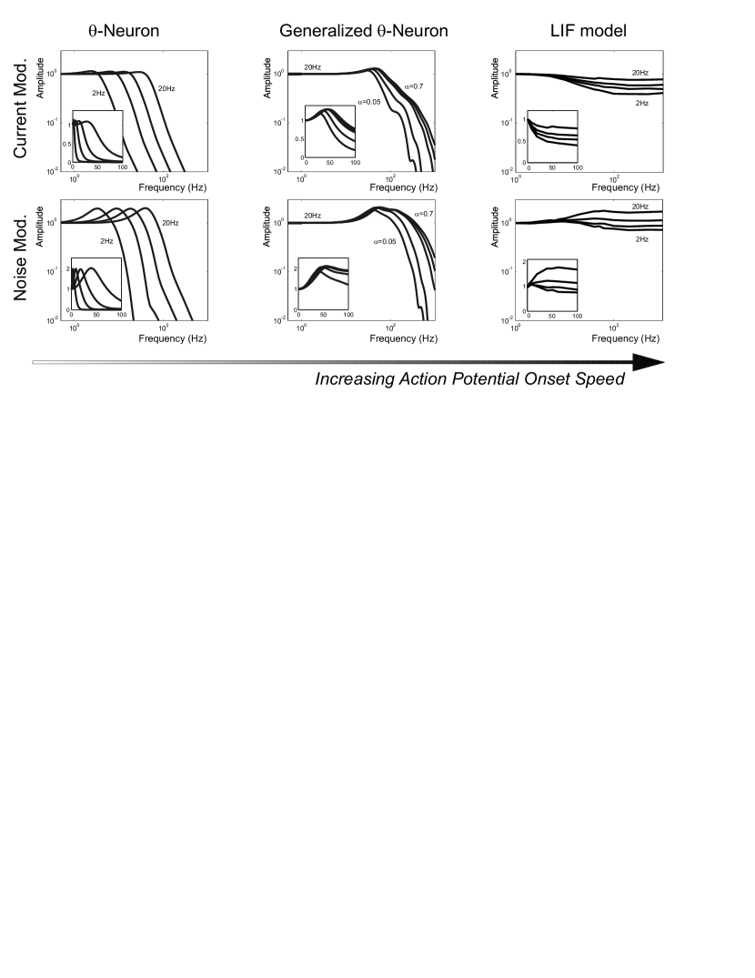
Figure 4: Response amplitude for increasing values of the action potential onset speed. In the left column the response of the $\theta$-neuron for modulations in the mean input current and the noise amplitude is shown for different values of the stationary firing rate. The response exhibits a cut-off behavior, frequencies larger than the stationary firing rate are strongly damped. The middle column shows the response of the generalized model for both types of modulation and a stationary rate of 20Hz. For increasing values of the action potential onset speed the response amplitude grows for frequencies in the interval from $100\textrm{Hz}$ to $1\textrm{kHz}$, while the resonance maximum only slightly shifts to larger frequencies. The response of the noise modulation is much larger in this interval than the response to modulations in the mean current. For comparison the right column shows the response of the leaky integrate-and-fire (LIF) model. The response amplitude does not decay for large frequencies, for modulations of the noise amplitude it can even grow with increasing input frequencies. Parameters in the LIF simulation are as in Brunel01 , except $\tau_{s}=10\textrm{ms}$, $\sigma=5\textrm{mV}$, $I_{0}=14.6;16.2;17.5;19.5\textrm{mV}$ for a mean firing rate of $2,5,10,20\textrm{Hz}$.

Using the matrix method described above, we computed the linear responses to modulations in the mean input current and to modulations in the noise amplitude. Figure 4 summarizes the response amplitude curves for the $\theta$-neuron model, the generalized $\theta$-neuron model and compares them to direct numerical simulations of the response of the leaky integrate-and-fire (LIF) model.

The $\theta$-neuron exhibits a cut-off behavior in its response amplitude to both types of input modulations. Frequencies up to the stationary firing rate can be transmitted unattenuated larger frequencies are strongly damped. For an increasing onset speed and fixed stationary rate the resonance maximum shifts only to slightly larger frequencies, a dramatic change, however, occurs at intermediate frequencies up to 1kHz. In this regime the response amplitude is substantially lifted to much larger transmission amplitudes. This effect is much more pronounced for the case of a modulation in the noise amplitude than for modulations in the mean input current, leading to an undamped response for frequencies up to 200Hz. The LIF model, on the other hand, shows a completely artificial response behavior. The transmission function, for both types of modulations does not decay at all, even for frequencies up to 1kHz. For modulations in the noise amplitude, the transmission function can even grow for increasing stimulation frequencies.

III.3 Nonlinear response for large stimulation amplitudes

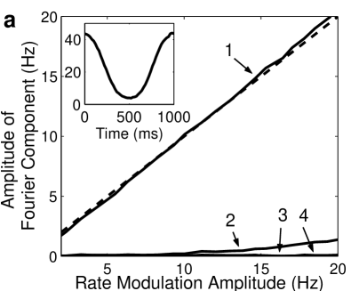
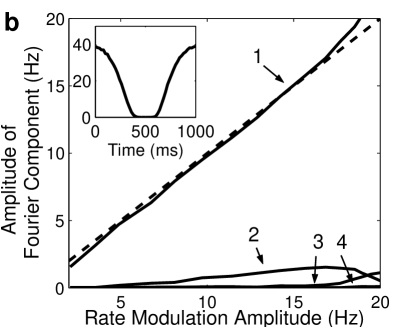
Figure 5: Amplitude of the first four Fourier components as a function of overall modulation amplitude of the population averaged firing rate for (a) modulations in the mean input current and (b) for modulations in the noise amplitude ($\alpha=0.7$). The mean output rate is 20Hz, the modulation frequency 1Hz. The dashed line is the diagonal. Up to amplitudes close to the mean output rate, the first Fourier component is indistinguishable from the diagonal, indicating that the response is essentially linear. Starting from amplitudes comparable to the mean rate, the influence of higher order Fourier components becomes substantial. The insets show the rate modulation for a modulation amplitude of 20Hz.

So far we have only considered the linear response transmission function, which is strictly speaking only valid in the limit in which the stimulation amplitude goes to zero. Here we show, however, that the linear response covers a large range of input amplitudes. In principle, we could use the same matrix method employed for the linear response theory, taking into account higher order Floquet modes Reichl88 . Here we explore this regime, however, by direct numerical simulation of Eq. (II.1). Figure 5 shows the amplitude of the first four Fourier modes of the rate response as a function of the overall amplitude of the rate modulation. For both types of modulations, the first Fourier component clearly dominates the response up to amplitudes close to the mean rate, where nonlinearities are naturally expected, as there are no negative firing rates. This demonstrates that the linear response theory, although rigorously valid for small modulation amplitudes only, predicts the response in a large dynamical range of input amplitudes.

IV Summary and Discussion

The dynamical response properties of the generalized $\theta$-neuron with adjustable AP onset speed were calculated in the presence of a fluctuating correlated background noise. Methodologically we introduced a new approach which is based on the expansion of the corresponding Fokker-Planck operator to a complete set of orthonormal functions, leading to a sparse matrix representation. We then computed the eigenvalues and eigenfunctions of this matrix using an iterative scheme, the Arnoldi method. The high frequency limit was calculated analytically. It turned out, that the response amplitude decays as $\omega^{-\gamma}$, where $\gamma$ depends on the kind of stimulation and, surprisingly, the phase at which a spike is emitted. As soon as this point differs from $\pi$, where the dynamics is insensitive to external inputs, the exponent $\gamma$ is $1$, giving the same asymptotic response behavior as conductance based neuron models. Using the eigenvalues and eigenfunctions we then presented a method to evaluate the dynamic response to small time-varying inputs. There we found that for the classical $\theta$-neuron model the response exhibits a cut-off behavior: For a modulation in the mean input current as well as for a modulation in the noise amplitude frequencies above the stationary rate of the neuron were strongly damped. In the generalized $\theta$-neuron the damping in the regime up to 1kHz is substantially reduced for both types of input modulations when the AP onset speed is increased, although the high frequency limit is the same as in the classical $\theta$-neuron. The response amplitude for the noise amplitude modulation is typically much larger than the response amplitude for the mean input modulation. The linear response theory, although only derived for small modulations of the input current turned out to be valid in a large dynamical range, which we demonstrated by direct numerical simulations. Amplitudes of the rate modulation up to the mean output rate turned out to be well described by the linear theory.

Simple phenomenological, yet dynamically realistic models of cortical neurons are of key importance for studies in theoretical neuroscience, starting from studies on spike timing to large scale network simulations or analytical network studies. While stationary response properties, such as mean firing rates or processes have been studied in many models, which operate on long time scales, e.g. adaptation (see e.g. Benda03 ; Senn03 ; Izhikevich04 ), studies on the dynamic response properties are rare. Most of these studies consider the dynamic response in the class of integrate-and-fire (IF) models Knight72 ; Brunel01 ; Lindner02 ; Fourcaud02 . In these studies, it was demonstrated that IF models can relay incoming stimuli instantaneously. Recently it was shown, however, that this response behavior strongly disagrees with the response of conductance based models and rather represents an oversimplification of the model than a feature of real neurons Naundorf03 ; Fourcaud03 . While in Naundorf03 the response properties of the classical $\theta$-neuron were investigated, the authors of Fourcaud03 studied another phenomenological neuron model, the EIF model, which mimics the dynamical response properties of a conductance based model. Our study corroborates and extends some of their results using a generalized model of the classical $\theta$-neuron Kopell86 ; Gutkin98 , a canonical model of conductance based neuron models, which exhibit type-I excitability and which, in contrast to IF models, incorporates a dynamic action potential onset. While the classical $\theta$-neuron model was originally studied in the super-threshold, noise-free caseErmentrout84 ; Kopell86 , recent studies focused on the response in the presence of fluctuating input currents Gutkin98 ; Lindner03 ; Brunel03 . These studies indicated that in a large parameter regime the $\theta$-neuron exhibits the same stationary response properties as cortical neurons, e.g. a realistic shape of the f-I curve and irregular firing in the subthreshold regime.

Despite these results, a major point of criticism questioning the biological relevance of the model, remained: While the $\theta$-neuron reflects the dynamics at the onset to repetitive firing, it lacks the sharp action potential upstroke found in more detailed conductance based models and real neurons Fourcaud03 . It was further argued that this deficiency results in a high frequency limit of the linear response amplitude, which decays too fast $\propto\omega^{-2}$, while the linear response amplitude in conductance neuron models only decays $\propto\omega^{-1}$. To address these issues we generalized the classical $\theta$-neuron, incorporating an adjustable AP onset speed, thereby mimicking the fast sodium activation at the action potential onset. Surprisingly, our study reveals that the high frequency limit, does not depend at all on the speed at the AP onset, but rather on the phase variable, at which action potentials are emitted. If at this point the dynamics is insensitive to external inputs, as in the classical $\theta$-neuron, the decay of the linear response amplitude is at least $\propto\omega^{-2}$, whereas the decay is always $\propto\omega^{-1}$ if the dynamics is not completely insensitive to external inputs, as is the case in conductance based neuron models. Moreover, the full transmission function reveals that the onset of the high-frequency limit can be shifted to very high frequencies if the speed of the AP onset is increased. These results question the relevance of the high frequency limit as a criterion for the typical transmission speed of neuron models.

For the computation of the linear response amplitude we did not resort to direct numerical simulations, but used a method based on the eigenfunctions and eigenvalues of the Fokker-Planck operator, describing the dynamics of the probability density function in the presence of a temporally correlated fluctuating input current. While this approach is in general well-known (see e.g. Risken96 and Knight00 ; Mattia02 for an application to the non-leaky integrate-and-fire model in the presence of an uncorrelated background noise), we derived a sparse matrix representation, for which we computed eigenvalues and eigenfunctions with very high numerical accuracy using a fast iterative scheme, the Arnoldi method Trefethen97 ; Lehoucq98 . Compared to previous studies on dynamical responses Brunel01 ; Fourcaud02 ; Fourcaud03 , this allowed for the computation of the linear response properties with an accuracy that would be hard to meet by a direct simulation of the single neuron dynamics.

Besides this, our results provide a direct link to experiments. In a recent study Brumberg02 it was shown that the AP width in neocortical neurons is strongly correlated with the critical frequency up to which a neuron can phase lock to sinusoidal input stimulations. This is indeed the same result we found for the generalized $\theta$-neuron: With increasing AP onset speed the response amplitude shifts to larger frequencies, enabling the model to respond to frequencies much larger than its own stationary rate. In a second experimental study it was demonstrated that cortical neurons subject to fluctuating input currents adapt their instantaneous firing much faster when stimulated with a step input in the noise amplitude than with a step mean input current Silberberg04 . This behavior is well reproduced by the generalized $\theta$-neuron. For increasing values of the AP onset speed, the response amplitude at high frequencies is one order of magnitude larger for the stimulation in the noise amplitude, compared to the stimulation in the mean input current. Both results strongly suggest that the generalized $\theta$-neuron, despite its simplicity and analytic tractability, captures well the essence of the AP generating mechanism of multidimensional conductance based neuron models. Future experimental studies will have to show to what extent the generalized $\theta$-neuron predicts the dependence of the dynamical response properties on the AP generating mechanism.

References

- (1) M. Abramowitz, and I.A. Stegun (1972). Tables of Mathematics Functions. New York: Dover Publications
- (2) Anderson JS, Lampl I, Gillespie DC, Ferster D. (2000). The contribution of noise to contrast invariance of orientation tuning in cat visual cortex. Science, 290, 1968-72
- (3) Benda J, Herz AV. (2003). A universal model for spike-frequency adaptation. Neural Comput., 15, 2523-64
- (4) Brumberg JC. (2002). Firing pattern modulation by oscillatory input in supragranular pyramidal neurons. Neuroscience, 114, 239-46
- (5) Brunel N, Hakim V. (1999). Fast global oscillations in networks of integrate-and-fire neurons with low firing rates., 11, 1621-71
- (6) Brunel N. (2000). Dynamics of sparsely connected networks of excitatory and inhibitory spiking neurons., 8, 183-208
- (7) Brunel N, Chance FS, Fourcaud N, Abbott LF. (2001). Effects of synaptic noise and filtering on the frequency response of spiking neurons. Phys Rev Lett., 86,2186-9
- (8) Brunel N, Latham PE. (2003). Firing rate of the noisy quadratic integrate-and-fire neuron. Neural Comput., 15, 2281-306
- (9) Coddington, E., & Levinson, N. (1955). Theory of ordinary differential equations. New York: McGraw-Hill.
- (10) Destexhe A, Pare D. (1999). Impact of network activity on the integrative properties of neocortical pyramidal neurons in vivo. J Neurophysiol., 81, 1531-47
- (11) Ermentrout, G., & Kopell, N. (1984). Frequency plateaus in a chain of weakly coupled oscillators, I. SIAM J. Math. Anal., 15, 215-237.
- (12) Ermentrout GB, Kopell N (1986). Parabolic bursting in an excitable system coupled with a slow oscillation. SIAM-J.-Appl.-Math., 2, 233-53
- (13) Fourcaud N, Brunel N. (2002). Dynamics of the firing probability of noisy integrate-and-fire neurons. Neural Comp., 14, 2057-110
- (14) Fourcaud-Trocmé N, Hansel D, van Vreeswijk C, Brunel N. (2003). How spike generation mechanisms determine the neuronal response to fluctuating inputs. J Neurosci., 23, 11628-40
- (15) C.W. Gardiner, Handbok of Stochastic Methods, (Springer, Berlin, 1985)
- (16) Gerstner, W. (2000). Population dynamics of spiking neurons: Fast transients, asynchronous states, and locking. Neural Computation, 12, 43-89.
- (17) Guckenheimer, J. (1975). Isochrons and phaseless sets. J. Math. Biol., 1, 259-273.
- (18) Gutkin BS, Ermentrout GB. (1998). Dynamics of membrane excitability determine interspike interval variability: a link between spike generation mechanisms and cortical spike train statistics. Neural Comput., 10, 1047-65
- (19) Izhikevich E.M. (2004). Which Model to Use for Cortical Spiking Neurons? IEEE Transactions on Neural Networks, In press
- (20) van Kampen NG (1981). Itô versus Stratonovich, J Stat Phys., 24, 175-87
- (21) Knight BW. (1972). Dynamics of encoding in a population of neurons. J Gen Physiol., 59, 734-66
- (22) Knight BW, Omurtag A, Sirovich L. (2000) The approach of a neuron population firing rate to a new equilibrium: An exact theoretical result. Neural Comp., 12, 1045-55
- (23) Lapicque L. (1907). Recherches quantitatives sur l’excitation electrique des nerfs traitee comme une polarization. J. Physiol. Pathol. Gen., 9, 620-635
- (24) Lehoucq R, Sorensen DC, Yang C. (1998). Arpack User’s Guide: Solution of Large-Scale Eigenvalue Problems With Implicitly Restarted Arnoldi Methods. SIAM, Philadelphia.
- (25) Lindner B, Schimansky-Geier L. (2002). Transmission of noise coded versus additive signals through a neuronal ensemble., Phys Rev Lett., 86, 2934-7
- (26) Lindner B, Longtin A, Bulsara A. (2003). Analytic expressions for rate and CV of a type I neuron driven by white gaussian noise. Neural Comput., 15, 1760-87
- (27) Mattia M, Del Giudice P. (2002). Population dynamics of interacting spiking neurons. Phys Rev E, 66, 051917
- (28) C. Morris and H. Lecar (1981). Voltage oscillations in the barnacle giant muscle fiber. Biophys. J. 35, 193
- (29) Naundorf B, Geisel T, Wolf F. (2003). The Intrinsic Time Scale of Transient Neuronal Responses. xxx.lanl.gov, physics/0307135, Preprint
- (30) Naundorf B, Geisel T, Wolf F. (2004). Dynamical Response Properties of a Canonical Model for Type-I Membranes. Neurocomp., In Press
- (31) L.E. Reichl (1988). Transitions in the Floquet Rates of a Driven Stochastic-System. J. Stat. Phys. 53, 41
- (32) H. Risken, The Fokker Planck Equation: Methods of Solution and Applications, (Springer, Berlin, 1996)
- (33) Rauch A, La Camera G, Luscher HR, Senn W, Fusi S. (2003). Neocortical pyramidal cells respond as integrate-and-fire neurons to in vivo-like input currents. J Neurophysiol., 90, 1598-612
- (34) Silberberg G, Bethge M, Markram H, Pawelzik K, Tsodyks M. (2004). Dynamics of population rate codes in ensembles of neocortical neurons. J Neurophysiol., 91, 704-9
- (35) Softky, W., Koch, K. (1993). The highly irregular ring of cortical cells is inconsistent with temporal integration of random EPSPs. J. Neurosci., 13, 334-55.
- (36) S. H. Strogatz. Nonlinear Dynamics and Chaos, Addison Wesley (1995)
- (37) T. Tateno, A. Harsch, H. P. Robinson. (2004). Threshold firing frequency-current relationships of neurons in rat somatosensory cortex: type 1 and type 2 dynamics., J Neurophysiol., 92, 2283-94
- (38) Trefethen NL, Bau D. (1997), Numerical Linear Algebra. Philadelphia: SIAM
- (39) Tuckwell H. (1988). Introduction to theoretical neurobiology (2 vols.). Cambridge: Cambridge University Press
- (40) Volgushev M, Eysel UT. (2000). Noise makes sense in neuronal computing. Science, 290, 1908-9
- (41) C. van Vreeswijk, H. Sompolinsky. (1996). Chaos in neuronal networks with balanced excitatory and inhibitory activity. Science, 274, 1724-6.
- (42) Wang XJ, Buzsaki G. (1996). Gamma oscillation by synaptic inhibition in a hippocampal interneuronal network model. J Neurosci., 16, 6402-13
- (43) Winfree, A. (1967). Biological rythms and behavior of pupulations of coupled oscillators. J. Theo. Biol., 16, 15
- (44) Winfree, A. (2001). The geometry of biological time. Second Edition. New York: Springer-Verlag.