Order independent structural alignment of circularly permuted proteins

Abstract–Circular permutation connects the N and C termini of a protein and concurrently cleaves elsewhere in the chain, providing an important mechanism for generating novel protein fold and functions. However, their in genomes is unknown because current detection methods can miss many occurances, mistaking random repeats as circular permutation. Here we develop a method for detecting circularly permuted proteins from structural comparison. Sequence order independent alignment of protein structures can be regarded as a special case of the maximum-weight independent set problem, which is known to be computationally hard. We develop an efficient approximation algorithm by repeatedly solving relaxations of an appropriate intermediate integer programming formulation, we show that the approximation ratio is much better then the theoretical worst case ratio of $r=1/4$. Circularly permuted proteins reported in literature can be identified rapidly with our method, while they escape the detection by publicly available servers for structural alignment.

Keywords–circular permuations, integer programming, linear programming, protein structure alignment

Introduction

A circularly permuted protein arises from ligation of the N and C termini of a protein and concurrent cleavage elsewhere in the chain [1, 2]. In nature, circular permutation often originate from tandem repeats via duplication of the C-terminal of one repeat together with the N-terminal of the next repeat, as is the case of swaposin. Another mechanism is ligation and cleavage of peptide chains during post-translational modification, as is the case of concanavalin A. The full extent of circular permutation and thier biological consequences are currently unknown. Discovery of circular permutation at genome wide scale will enable systematic studies of its contribution to the generation of novel protein function and novel protein fold.

Currently, sequence alignment based methods are the only available tools for detecting circular permutations. These include postprocessing output from standard dynamic programming methods, as well as customized algorithms [3]. Sequence based methods can miss many circularly permuted proteins, because either one or both fragments may escape detection by local alignment if the two proteins are distantly related.

Protein structures are far more conserved than sequences, and they can reveal very distant evolutionary relationship [4]. Jung et. al. [5] showed that there is potential to discover remotely related protein domains by artifically permutating proteins and superimposing them on native domains in the protein structure database. Detecting circular permutation from structures has the promise to uncover many more ancient permutation events that escape sequence methods.

In this study, we describe a new algorithm for detecting circular permutation in protein structures. We show with examples that our algorithm can align circular permutations reported in literature. Our work introduces an efficient approximate method for protein substructure comparison. Two protein structures are first cut into pieces exhaustively of varying lengths and then compared. An approximation algorithm is used to search for optimal combination of peptide pieces from both structures. With the special nature of spatial distribution of proteins, a fractional version of local-ratio approach for scheduling split-interval graphs works well for detecting very similar spatial substructures. Our experimentation showed that the approximation ratio is excellent, with an average value of at least $1/2.53$.

Structural Alignment of Circularly Permuted Proteins

Three simplified protein structures that are related by circular permutation are shown in Figure 1. The three corresponding domains (labeled A, B, and C, respectively) are all very similar across proteins. The global spatial arrangements of these three domains are also very similar. However, the orderings of these domains in primary sequence are completely different.

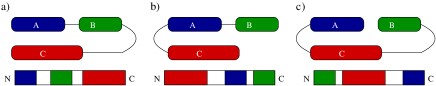
Figure 1: Three cartoon protein structures related by a circular permutation. The location of domains A,B,C are shown in a primary sequence layout below each structure.

The discontinuity and different ordering of spatially neighboring domains in primary sequence makes the detection of global structural similarity. Most structural alignment methods are unable to connect the break where circular permutation occurs, and would prematurely terminates the alignment. In addition, the reverse ordering of residues within a domain between two proteins also poses challenge for such methods. For example, the A domain in Figure 1a is ordered from N to C. The same domain in Figure 1b is ordered from C to N. The algorithm outlined below is well-suited to solve these types of challenging problems.

Basic Methodology

We first introduce some notations: A substructure $\lambda_{a}$ of a protein structure $\mathcal{S}_{a}$ is a continuous fragment $\lambda_{a}=(a_{1},a_{2})\in\Lambda_{a}$, where $a_{1},a_{2}$ are the residue numbers of the beginning and end of the substructure, respectively, and $1\leq a_{1}<a_{2}\leq|\mathcal{S}_{a}|$. A residue $t\in\lambda_{a}$ is part of substructure $\lambda_{a}$ if $a_{1}\leq t\leq a_{2}$. $\Lambda_{a}$ is the set of all possible continuous substructures or fragments of protein structure $\mathcal{S}_{a}$, i.e., $\Lambda_{a}=\{(a_{1},a_{2})\}$. $\mathcal{S}_{b},\lambda_{b},b_{1},b_{2}$, and $\Lambda_{b}$ are similarly defined.

The problem of protein substructure comparison is captured in the following Basic Substructure Similarity Identification (BSSI_Λ,σ) problem.

Definition 1

Instance:

a set $\Lambda\subseteq\Lambda_{a}\times\Lambda_{b}$ of ordered pairs of substructures of $\mathcal{S}_{1}$ and $\mathcal{S}_{2}$ and a similarity function $\sigma:\Lambda\rightarrow{{R}_{+}}$ mapping these pairs of substructures to similarity values (non-negative real numbers).

Valid solutions:

a set $\{\lambda_{1},\lambda_{2},\cdots,\lambda_{k}\}=\{(\lambda_{a,1},\lambda_{b,1}),(\lambda_{a,2},\lambda_{b,2}),\cdots,(\lambda_{a,k},\lambda_{b,k})\}$ of pairs of substructures such that $\lambda_{\ell,i}\in\Lambda_{\ell}$ and $\lambda_{\ell,j}\in\Lambda_{\ell}$ are disjoint for $\ell\in\{a,b\}$ and $i\neq j$.

Objective:

maximize the total similarity of the selection $\sum_{i=1}^{k}\sigma(\lambda_{a,i},\lambda_{b,i})$.

The BSSI_Λ,σ problem is a special case of the famous maximum-weight independent set (MWIS) problem in graph theory [6]. BSSI_Λ,σ is MAX-SNP-hard even when the substructures are restricted to short lengths [7]. Our approach is to adopt the approximation algorithm for scheduling split-interval graphs [7], which is based on a fractional version of the local-ratio approach. We introduce the following definitions:

• The conflict graph $G_{\Delta}=(V_{\Delta},E_{\Delta})$ for any subset $\Delta\subseteq\Lambda$, is a graph in which $V_{\Delta}=\Delta$ and $E_{\Delta}$ consists of all distinct pairs of vertices $\{(\lambda_{a},\lambda_{b}),(\lambda_{a}^{\prime},\lambda_{b}^{\prime})\}$ from $V_{\Delta}$ such that $\lambda_{i}$ and $\lambda_{i}^{\prime}$ are not disjoint for some $i\in\{a,b\}$.

• The closed neighborhood of a vertex $v$ of $G_{\Delta}$, denoted by Nbr${}_{\Delta}[v]$, is defined as $\{u\;|\;\{u,v\}\in E_{\Delta}\}\cup\{v\}$.

The recursive algorithm for solving BSSI_Λ,σ is as follows:

Table I: The LP formulation of the BSSI problem.

Maximize $\;\;\;\;\sum_{\lambda\in\Lambda}\sigma(\lambda)\cdot x_{\lambda}$
subject to
$\displaystyle\sum_{t\in\lambda_{a}\in\Lambda_{a}\;\&\;\lambda=(\lambda_{a},\lambda_{b})\in\Lambda}\par y_{\lambda,\lambda_{a}}\leq 1$	$\forall t\in\Lambda_{a}$	(1)
$\displaystyle\sum_{t\in\lambda_{b}\in\Lambda_{b}\;\&\;\lambda=(\lambda_{a},\lambda_{b})\in\Lambda}\par y_{\lambda,\lambda_{b}}\leq 1$	$\forall t\in\Lambda_{b}$	(2)
$y_{\lambda,\lambda_{a}}-x_{\lambda}\geq 0$	$\forall\lambda=(\lambda_{a},\lambda_{b})\in\Lambda$	(3)
$y_{\lambda,\lambda_{b}}-x_{\lambda}\geq 0$	$\forall\lambda=(\lambda_{a},\lambda_{b})\in\Lambda$	(4)
$x_{\lambda},y_{\lambda,\lambda_{a}},y_{\lambda,\lambda_{b}}\geq 0$	$\forall\lambda=(\lambda_{a},\lambda_{b})\in\Lambda$	(5)

• Remove every substructure pairs $\lambda=(\lambda_{a},\lambda_{b})\in\Lambda$ such that $\sigma(\lambda_{a},\lambda_{b})\leq 0$. If $\Lambda=\emptyset$ after these removals, then return $\emptyset$ as the solution.

• Solve a linear programming (LP) formulation of the BSSI_Λ,σ problem by relaxing a corresponding integer programming version of the BSSI_Λ,σ problem. For every $\lambda=(\lambda_{a},\lambda_{b})\in\Lambda$, introduce three indicator variables $x_{\lambda}$, $y_{\lambda,\lambda_{a}}$ and $y_{\lambda,\lambda_{b}}\in\{0,1\}$, but relaxed to real numbers. The LP formulation is shown in Table I.

• For every vertex $\lambda\in\Lambda$ of $G_{\Lambda}$, compute its local conflict number $\displaystyle\alpha_{\lambda,\Lambda,\sigma}=\sum_{\mu\in\mbox{Nbr}_{\Lambda}[\lambda]}x_{\mu}$. Let $\lambda_{\rm min}$ be a vertex with the minimum local conflict number $r_{\Lambda,\sigma}=\min_{\lambda}\{\alpha_{\lambda,\Lambda,\sigma}\}$. Define a new similarity function $\sigma_{\rm new}$ from $\sigma$ as follows $\sigma_{\rm new}(\lambda)=\left\{\begin{array}[]{ll}\sigma(\lambda),&\mbox{if $v\not\in\mbox{Nbr}_{\Lambda}[\lambda_{\rm min}]$}\\ \sigma(\lambda)-\sigma(\lambda_{\rm min}),&\mbox{otherwise}\\ \end{array}\right.$.

• Recursively solve the BSSI${}_{\Lambda,\sigma_{\rm new}}$ problem using the same approach. Let $\Lambda^{\prime}\subseteq\Lambda$ be the solution returned.

• If the substructure pair $\lambda_{\rm min}$ can be selected together with all the pairs in $\Lambda^{\prime}$ then return $\Lambda^{\prime}\cup\{\lambda_{\rm min}\}$ as the solution, else return $\Lambda^{\prime}$ as the solution.

A brief explanation of the various inequalities in the LP formulation as described above is as follows:

• The interval clique inequalities in (1) (resp. (2)) ensures that the various substructures of $\mathcal{S}_{a}$ (resp. $\mathcal{S}_{b}$) in the selected pairs of substructures from $\Lambda$ are mutually disjoint.

• Inequalities in (3) and (4) ensure consistencies between the indicator variable for substructure pair $\lambda$ and its two substructures $\lambda_{a}$ and $\lambda_{b}$.

• Inequalities in (5) ensure non-negativity of the indicator variables.

In implementation, the graph $G_{\Delta}$ is considered implicitly via intersecting intervals. The interval clique inequalities can be generated via a sweepline approach. The running time depends on the number of recursive calls and the times needed to solve the LP formulations. Let LP$(n,m)$ denote the time taken to solve a linear programming problem on $n$ variables and $m$ inequalities. Then the worst-case running time of the above algorithm is $O(|\Lambda|\cdot\mbox{LP}(3|\Lambda|,5|\Lambda|+|\Lambda_{1}|+|\Lambda_{2}|))$. However, the worst-case time complexity happens under the excessive pessimistic assumption that each recursive call removes exactly one vertex of $G_{\Delta}$, namely $\lambda_{\rm min}$ only, from consideration, which is unlikely to occur in practice as our computational results show.

The performance ratio of our algorithm is as follows. Let $r$ be the maximum of all the $r_{\Lambda,\sigma}$’s in all the recursive calls. Proofs in [7] translate to the fact that $r\leq 4$ and the above algorithm returns a solution whose total similarity is at least $1\over r$ times that of the optimum. The value of $r$ is much smaller compared to $4$ in practice (e.g., $r=2.53$).

Implementation and Computational Details.

We present a simplified example for illustration two protein structures $\mathcal{S}_{a}$ (Figure 2a) and $\mathcal{S}_{b}$ (Figure 2a) are selected for alignment. Here $\mathcal{S}_{b}$ is the structure to be aligned to the reference structure $\mathcal{S}_{a}$. We systematically cut $\mathcal{S}_{b}$ into fragments of length 7–25 and exhaustively compute a similarity score of each fragment from $\mathcal{S}_{b}$ to all possible fragments of equal length in $\mathcal{S}_{a}$. Each fragment pair can be thought of as a vertex in a graph, as shown in Figure 2b.

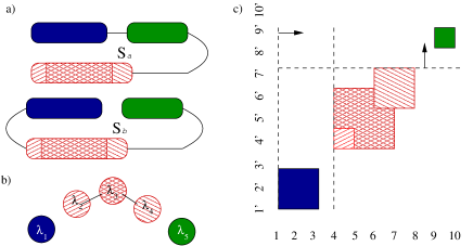
Figure 2: A simplified representation of the Basic Substructure Similarity Identification problem: a) The cartoon representation of circularly permuted proteins $\mathcal{S}_{a}$ and $\mathcal{S}_{b}$, b) The problem represented as a graph where each node, $\lambda$, represents an aligned fragment pair and each edge represents a conflict, where the same residues are contained in different fragments and c) An illustration how sweep lines (dashed) can identify overlapping aligned pairs.

Suppose we have the following similarity scores for aligned substructures: $\sigma(\lambda_{1})=\sigma((1,3)(1^{\prime},3^{\prime}))=8,\sigma(\lambda_{2})=\sigma((4,5)(4^{\prime},5^{\prime}))=5,\sigma(\lambda_{3})=\sigma((4,7)(4^{\prime},7^{\prime}))=7,\sigma(\lambda_{4})=\sigma((6,8)(6^{\prime},8^{\prime}))=3,\mbox{ and }\sigma(\lambda_{5})=\sigma((9,10)(9^{\prime},10^{\prime}))=6.$

We can describe the problem of selecting the best structural fragment pairs as to maximize $8x_{\lambda_{1}}+5x_{\lambda_{2}}+7x_{\lambda_{3}}+3x_{\lambda_{4}}+6x_{\lambda_{5}}$.

Figure 2b shows the conflict graph for the set of fragments. A sweep line (shown as dashed lines in Figure 2c) is implicitly constructed ($O(n)$ time after sorting) to determine which vertices of fragment pair overlap. A conflict is shown in Figure 2b as edges between vertices. Vertices $\lambda_{1}$ and $\lambda_{5}$ do not conflict with any other fragments, while $\lambda_{2}$ and $\lambda_{4}$ conflict with $\lambda_{3}$. For this graph, the constraints in the linear programming formulation are shown in Table II. The linear programming problem is solved using the Bpmpd package [8].

Table II: The constraints of the consflict graph for the set of fragments in Figure 2c.

Interval Clique inequality:		(1)
$y_{\lambda_{1},\lambda_{a}}\leq 1$	Line sweep at 1
$y_{\lambda_{2},\lambda_{a}}+y_{\lambda_{3},\lambda_{a}}\leq 1$	Line sweep at 4, 5
$y_{\lambda_{3},\lambda_{a}}+y_{\lambda_{4},\lambda_{a}}\leq 1$	Line sweep at 6, 7
$y_{\lambda_{4},\lambda_{a}}\leq 1$	Line sweep at 8
$y_{\lambda_{5},\lambda_{a}}\leq 1$	Line sweep at 9
Interval Clique inequality:		(2)
$y_{\lambda_{1},\lambda_{b}}\leq 1$	Line sweep at 1’
$y_{\lambda_{2},\lambda_{b}}+y_{\lambda_{3},\lambda_{b}}\leq 1$	Line sweep at 4’, 5’
$y_{\lambda_{3},\lambda_{b}}+y_{\lambda_{4},\lambda_{b}}\leq 1$	Line sweep at 6’, 7’
$y_{\lambda_{4},\lambda_{b}}\leq 1$	Line sweep at 8’
$y_{\lambda_{5},\lambda_{b}}\leq 1$	Line sweep at 9’
Interval Clique inequalities:		(3, 4)
$y_{\lambda_{1},\lambda_{a}}-y_{\lambda_{1}}\geq 0$,	$y_{\lambda_{1},\lambda_{b}}-y_{\lambda_{1}}\geq 0$
$y_{\lambda_{2},\lambda_{a}}-y_{\lambda_{2}}\geq 0$,	$y_{\lambda_{2},\lambda_{b}}-y_{\lambda_{2}}\geq 0$
$y_{\lambda_{3},\lambda_{a}}-y_{\lambda_{3}}\geq 0$,	$y_{\lambda_{3},\lambda_{b}}-y_{\lambda_{3}}\geq 0$
$y_{\lambda_{4},\lambda_{a}}-y_{\lambda_{4}}\geq 0$,	$y_{\lambda_{4},\lambda_{b}}-y_{\lambda_{4}}\geq 0$
$y_{\lambda_{5},\lambda_{a}}-y_{\lambda_{5}}\geq 0$,	$y_{\lambda_{5},\lambda_{b}}-y_{\lambda_{5}}\geq 0$

The algorithm guarantees that there is a vertex $\lambda_{i}$ that satisfies $x_{\lambda_{i}}+\sum_{\lambda_{j}\in\mbox{Nbr}[\lambda_{i}]}{x_{\lambda_{j}}\leq 4},$ and all vertices are searched to find such a vertex. We then update $\sigma(\lambda_{j})$ for vertices that are neighbors of $\lambda_{i}$: $\sigma_{\mbox{new}}(\lambda_{j})=\sigma(\lambda_{j})-\sigma(\lambda_{i}),\quad\quad\mbox{ if $\lambda_{j}\in\mbox{Nbr}[\lambda_{i}]$}$ Vertices that have no neighbors, such as $\lambda_{1}$ and $\lambda_{5}$ in our example, are included in our final solution. Using the updated values of $\sigma(\lambda_{i})$, we remove vertices of substructure pairs that have score less than 0, and recursively solve the (smaller) LP problem again. The selected final set of fragments are then used to construct a substructure of $\mathcal{S}_{b}$. They are then aligned structurally by minimizing cRMSD.

Similarity score.

The similarity score $\sigma(\lambda)=\sigma(\lambda_{a},\lambda_{b})$ between two aligned substructures $\lambda_{a}$ and $\lambda_{b}$ is a weighted sum of a shape similarity value derived from cRMSD value and a sequence composition score (SCS): $\mbox{SCS}=\sum_{i=1}^{N}{B(A_{a,i},A_{b,i})},$ where $A_{a,i}$ and $A_{b,i}i$ are the amino acid residue type at aligned position $i$, $N$ the number of residues in the aligned fragment, and $B(A_{a,i},A_{b,i})$ the similarity score between $A_{a,i}$ and $A_{b,i}$ by the modified Blosum50 matrix, in which a constant is added to all entries such that the smallest entry is 1.0. The similarity score $\sigma(\lambda_{a},\lambda_{b})$ is calculated as follows:

$$\sigma(\lambda_{a},\lambda_{b})=\frac{\alpha(C-\mbox{cRMSD})+\beta(\mbox{SCS})}{N},$$

For the current implementation, $C=60,\alpha=6$, and $\beta=1$.

To improve computational efficiency, a threshold measure is introduced to immediately exclude low scoring fragment pairs from further consideration. Only fragment pairs scoring above the threshold will be candidates to be included in the final solution. In the above example, we assume that only fragment pairs represented by vertices $\lambda_{1}$, $\lambda_{2}$, $\lambda_{3}$, $\lambda_{4}$, and $\lambda_{5}$ (Figure 2b) are above the threshold.

Results

We discuss the structural alignments of several well known examples of naturally occurring circularly permuted proteins.

The results including other examples are summarized in Table III, which includes two additional examples of experimentally constructed human-made permuted proteins. None of them are found by existing servers.

Table III: Results from the structural alignment of circularly permuted protein, where $N$ equal the number of aligned residues in the final solution. Human-made circularly permuted proteins are listed at the bottom separated by a line from naturally occurring proteins.

PDB/Size	PDB/Size	Frag-	$N$	cRMSD
		ments
1rin/180	2cna/237	3	45	0.877
1rsy/121	1qas/123	4	44	1.107
1nkl/78	1qdm/74	6	48	1.832
1onr/316	1fba/360	7	77	2.444
1aqi/191	1boo/259	4	66	3.571
1avd/123	1swg/112	6	66	0.815
1gbg/214	1ajk/212	5	110	0.347

The first naturally occurring circular permutation was found in concanavalin A. and lectin favin. The structures of lectin from garden pea (1rin) and concanavalin A (2cna) (Figure 3a,b). In the structural alignment, three fragments align over 45 residues with a root mean square distance of 0.82Å. The superposition based on the aligned fragments is shown in Figure 3b. The residues spanning a break in the backbone due to the permutation are highlighted in red.

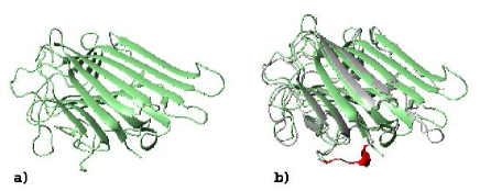
Figure 3: The structure of concanavalin A (2cna) (a) and its superposition to lectin from garden pea (1rin) (shown in gray) (b). The residues spanning the break due to the circular permutation are highlighted in red.

Discussion

The approximation algorithm introduced in this work can find good solutions for the problem of detecting circular permuted proteins. In contrast to methods based on sequence alignment alone, the ability to incorporate both structural and sequence similarity is critical. An experimentation in the alignment of 1rin and 2cna illustrates this point. After turning off the contribution from cRMSD in the similarity function $\sigma(\lambda_{a},\lambda_{b})$ by setting $\alpha=0$, we find altogether 452 fragments that score in the top 10% of the set of all SCS scores. This number is too large as the size of the conflict graph will be large. This makes subsequent comparison very difficult. Similarly, cRMSD measurement alone is inadequate for comparison. When matching fragments from 1rin and 2cna, we find there are 287 fragments that can be aligned with an cRMSD value $<3.0$ Åafter setting $\beta=0$. The use of composite similarity function is therefore essential to reduce false positives in substructure alignments.

In our method, scoring function plays pivotal role in detecting substructure similarity of proteins. Much experimentations are needed to optimize the similarity scoring system for general sequence order independent structural alignment. A necessary ingredient for a fully automated search of circular permuted proteins in database is a statistical measurement of significance of matched substructures. Since cRMSD measurement and therefore $\sigma(\lambda_{a},\lambda_{b})$ strongly depends on the length of matched parts and the gaps of the sequence break, a statistical model assessing the $p$-value of a measured $\sigma(\lambda)$ against a null model needs to be developed. Circular permutations that are likely to be biologically significant can then be automatically declared [4].

References

- [1] Y. Lindqvist and G. Schneider. Circular permutations of natural protein sequences: structural evidence. Curr. Opinion Struct. Biol., 7:422–427, 1997.
- [2] R.B. Russell and C.P. Ponting. Protein fold irregularities that hinder sequence analysis. Curr. Opinion Struct. Biol., 8:364–371, 1998.
- [3] S. Uliel, A. Fliess, A. Amir, and R. Unger. A simple algorithm for detecting circular permutations in proteins. Bioinformatics, 15(11):930–936, 1999.
- [4] T.A. Binkowski, L. Adamian, and J. Liang. Inferring functional relationship of proteins from local sequence and spatial surface patterns. J. Mol. Biol., 332:505–526, 2003.
- [5] J. Jung and B.K. Lee. Circularly permuted proteins in the protein structure database. Protein Science, 10:1881–1886, 2001.
- [6] N. Alon, U. Feige, A. Wigderson, and D. Zuckerman. Derandomized graph products. Computational Complexity, 5:60–75, 1995.
- [7] R. Bar-Yehuda, M.M. Halldörsson, J. Naor, H. Shachnai, and I. Shapira. Scheduling split intervals. In 14th ACM-SIAM Symposium on Discrete Algorithms, pages 732–741, 2002.
- [8] C.S. Mészáros. Fast Cholesky factorization for interior point methods of linear programming. Comp. Math. Appl., 31:49 – 51, 1996.