Rate-dependent propagation of cardiac action potentials in a one-dimensional fiber

Abstract

Action potential duration (APD) restitution, which relates APD to the preceding diastolic interval (DI), is a useful tool for predicting the onset of abnormal cardiac rhythms. However, it is known that different pacing protocols lead to different APD restitution curves (RCs). This phenomenon, known as APD rate-dependence, is a consequence of memory in the tissue. In addition to APD restitution, conduction velocity restitution also plays an important role in the spatiotemporal dynamics of cardiac tissue. We present new results concerning rate-dependent restitution in the velocity of propagating action potentials in a one-dimensional fiber. Our numerical simulations show that, independent of the amount of memory in the tissue, waveback velocity exhibits pronounced rate-dependence and the wavefront velocity does not. Moreover, the discrepancy between waveback velocity RCs is most significant for small DI. We provide an analytical explanation of these results, using a system of coupled maps to relate the wavefront and waveback velocities. Our calculations show that waveback velocity rate-dependence is due to APD restitution, not memory.

I INTRODUCTION

When a cardiac cell is depolarized by an electrical stimulus, it exhibits a prolonged elevation of transmembrane potential known as an action potential. We define the action potential duration (APD) as the time required for the cell to achieve 80% repolarization following a depolarizing stimulus. The refractory period between the end of an action potential the application of a subsequent stimulus is called the diastolic interval (DI). It is known that APD restitution (the dependence of the APD on preceding DI) is of fundamental importance in paced cardiac dynamics. In particular, studies ND ; GUEVARA show that the slope of the APD restitution curve (RC) is linked to the onset of alternans, an abnormal cardiac rhythm characterized by long-short variation of APD, which may lead to ventricular fibrillation and sudden cardiac death KARMA94 ; ROSENBAUM ; WATANABE-OG .

Experimental BOYETT ; ELHARRAR ; FRANZ and analytical TSGK investigations have shown that different pacing protocols lead to different APD RCs, a phenomenon known as APD rate-dependence. Several studies GULRAJANI ; CHIALVO ; OTANI indicate that the origin of APD rate-dependence is the presence of memory in cardiac tissue. That is, APD depends not only upon the preceding DI but also on the previous history of paced cardiac tissue. Memory appears to be a generic feature of cardiac muscle since it has been reported in humans FRANZ and various animals ELHARRAR ; HBG ; GETTES ; GIBBS .

Testing for rate-dependence involves the use of multiple pacing protocols and comparison of the resulting RCs. Two of the most commonly used pacing schemes are the dynamic and S1-S2 pacing protocols. Under the dynamic (steady-state) protocol, pacing is performed at a constant basic cycle length $B$ until steady-state is reached (no beat-to-beat variation in APD or DI). After recording the steady-state DI-APD pair, $B$ is changed by an amount $\Delta$ and the process is repeated. The dynamic RC is constructed by plotting all steady-state DI-APD pairs obtained from the dynamic pacing protocol over a range of $B$ values. The S1-S2 (standard) protocol also begins with pacing at a fixed basic cycle length $B$ (S1 interval) until steady-state is reached. Then, an S2 stimulus is applied at an interval $B_{1}$ after the final S1 stimulus. Setting $\delta=B_{1}-B$, the S1-S2 RC is obtained by plotting the APD following the S2 stimulus versus the preceding DI for different values of $\delta$. Note that there is only one dynamic RC, whereas each different S1 pacing interval can yield a distinct S1-S2 RC. For the purposes of this paper, we obtain only local S1-S2 RCs ($|\delta|$ small relative to S1) for different values of the S1 interval. In particular, following KALB we apply one short $(B_{1}=B-\delta)$ and one long $(B_{1}=B+\delta)$ perturbation at each different value of $B$.

The connection between rate-dependent APD restitution and memory is illustrated in Fig. 1, which shows APD RCs obtained from numerical simulations using two different ionic models (see Section II) of the cell membrane. Figure 1a is generated using a two-current model KARMA93 ; MS with no memory: the dynamic and S1-S2 RCs are indistinguishable. Figure 1 is generated using a three-current ionic model FK ; TSGM with some memory. One can see from Fig. 1b that segments of S1-S2 RCs (dashed curves) do not coincide with the dynamic RC (solid curve) for small DI values. The splitting between the dynamic and S1-S2 RCs is the manifestation of APD rate-dependence.

Figure 1: Typical APD restitution curves obtained using dynamic and S1-S2 pacing protocols ($\Delta=40$ ms, $\delta=\pm 20$ ms) for two different ionic membrane models. (a) A two-current model. (b) A three-current model. The dynamic RC (solid) and local S1-S2 RCs (dashed) are shown for different values of S1.

In the case of a network of electrically-coupled cardiac cells, conduction-velocity restitution also plays an important role in dynamics of the spatially extended system BANVILLE ; CKG . Indeed, when a sequence of propagating pulses is produced, both APD and the propagation speed of a pulse are influenced by the preceding pulse. Conduction-velocity restitution is analogous to APD restitution in that it relates the speed of an action potential at a given site to the DI at that site. Several authors CKG ; COURTEMANCHE ; FENTON-CHE have noted that abrupt changes in the pacing rate lead to discrepancies between the wavefront and waveback velocities. For this reason, we will always distinguish between wavefront (or activation front) velocity and waveback (or recovery front) velocity of propagating action potentials.

In this paper, we investigate rate-dependence of wavefront and waveback velocities of propagating action potentials in a one-dimensional fiber of cardiac cells. Using numerical simulations of different ionic membrane models (with and without memory) we demonstrate that the waveback velocity exhibits pronounced rate-dependence and the wavefront velocity does not (Section II). We derive an analytical relationship between wavefront and waveback velocities by modeling cardiac dynamics using a system of coupled maps with an arbitrary amount of memory. We show that APD restitution, not memory, leads to waveback velocity rate-dependence (Section III). We provide conclusions and discussion in Section IV. An Appendix on the two-current ionic model is included for reference.

II Rate-dependent velocity: numerical results

Typically, the cardiac action potential is modeled by considering ionic currents that flow across the cell membrane via ion channels. The rate-of-change of the transmembrane voltage is obtained by summing all ionic currents and dividing by the membrane capacitance. The ion channels act as gates that regulate the permeabilities of ions, most notably sodium, potassium and calcium. Hence, ionic models are presented as systems of ordinary differential equations that govern transmembrane voltage and gate variables.

In the case of a one-dimensional fiber, electrical coupling can be modeled by the inclusion of a diffusion term. The result is a reaction-diffusion partial differential equation known as the cable equation:

$$\frac{\partial v}{\partial t}=\kappa\frac{\partial^{2}v}{\partial x^{2}}-\frac{I_{\mathrm{total}}}{C_{m}}\hskip 28.45274pt0\leq x\leq L,$$ (1)

where $v$ denotes transmembrane voltage, $x$ measures distance from the stimulus site, $C_{m}$ is membrane capacitance, $\kappa$ is a diffusion coefficient, and $I_{\mathrm{total}}$ is the sum of all ionic currents. The number of currents varies depending upon the complexity of the ionic model. The diffusion coefficient incorporates membrane capacitance, cell surface-to-volume ratio, and longitudinal resistivity of cardiac muscle tissue. In all of our numerical simulations $C_{m}=\mathrm{1\>\mu F\>cm^{-2}}$ and $\kappa=\mathrm{0.001\>cm^{2}\>ms^{-1}}$. Neumann boundary conditions $v_{x}(0,t)=v_{x}(L,t)=0$ are imposed at both ends of the cable.

To investigate rate-dependent propagation, we perform numerical simulations of Eq. (1). We apply both dynamic and S1-S2 pacing protocols at one end of a cable, and measure the wavefront and waveback velocities of each propagating pulse. By analogy with APD rate-dependence, velocity rate-dependence means that different pacing protocols lead to different velocity RCs.

Since memory is responsible for APD rate-dependence, it is natural to hypothesize that memory also leads to wavefront and waveback velocity rate-dependence. Consequently, we use two different ionic models in our numerical simulations: a two-current ionic model MS with no memory and a three-current ionic model TSGM with some memory.

The details of the numerical experiments are as follows. Using a cable of length $L=10\>\mathrm{cm}$, we solve Eq. (1) numerically with an operator-splitting method. Stimuli are applied over a 1 mm region at the proximal ($x=0$) end of the fiber using both the dynamic and S1-S2 protocols described in the Introduction. In all simulations, we use $\Delta=40$ ms and $\delta=\pm 20$ ms. Pacing results in a train of pulses that propagate left-to-right in the fiber. Measurements of DI, APD, wavefront speed, and waveback speed are taken at $x=2.5\>\mathrm{cm}$. The position of a pulse wavefront is defined as the $x$ value for which the transmembrane voltage is $-60\mathrm{mV}$ and $dv/dx<0$. Likewise, waveback position is defined as the $x$ value at which $v=-60\mathrm{mV}$ and $dv/dx>0$. Linear interpolation is used to improve tracking of wavefront and waveback positions. Speeds are then computed by recording the time required for wavefronts and wavebacks to traverse a 1-mm-wide interval centered at $x=2.5\>\mathrm{cm}$. For illustration purposes, Fig. 2 shows a projection of a steady-state solution of Eq. (1) (with two-current ionic model) onto the $xt$ plane. Different shades of grey correspond to different transmembrane voltages, with black corresponding to the rest potential. Note that, in steady-state, projecting the wavefronts and wavebacks onto the $xt$ plane forms a sequence of parallel lines.

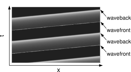
Figure 2: Steady-state space-time response obtained by numerical simulation of Eq. (1) with the two-current ionic model.

Results of numerical simulations of Eq. (1) with the two-current ionic model (no memory) are presented in Fig. 3, which shows wavefront (Fig. 3a) and waveback (Fig. 3b) velocity RCs. One can see from Fig 3a that the wavefront velocity RCs resulting from different pacing protocols are indistinguishable. Thus, there is no significant rate-dependence if velocities are measured at the wavefront. However, one can see from Fig 3b that segments of S1-S2 waveback velocity RCs (dashed curves) do not coincide with the dynamic waveback velocity RC (solid curve). As in the case of APD rate-dependence (see Fig. 1), the splitting between waveback velocity RCs is more pronounced for small values of DI.

Wavefront and waveback velocity RCs obtained from numerical simulations of a cable with the three-current ionic model (that has some memory) are presented in Fig. 4. The results are qualitatively similar to the two-current model results shown in Fig. 3.

There are two important points that we wish to emphasize. First, rate-dependent waveback velocity restitution does not depend upon the presence of memory in the tissue, as evidenced by our two-current model simulations. Second, rate-dependent waveback velocity is more pronounced for small values of $DI$. In what follows, we provide an analytical explanation of these findings.

Figure 3: Wavefront and waveback velocity RCs obtained from numerical simulation of Eq. (1) with two-current ionic model ($\Delta=40\>\mathrm{ms}$, $\delta=\pm 20\>\mathrm{ms}$). Velocities were measured at $x=2.5\>\mathrm{cm}$. (a) Wavefront velocity RCs. (b) Waveback velocity RCs. The dynamic RC is solid and the local S1-S2 RCs are dashed.

Figure 4: Wavefront and waveback velocity RCs obtained from numerical simulation of Eq. (1) with three-current ionic model ($\Delta=40\>\mathrm{ms}$, $\delta=\pm 20\>\mathrm{ms}$). Velocities were measured at $x=2.5\>\mathrm{cm}$. (a) Wavefront velocity RCs. (b) Waveback velocity RCs. The dynamic RC is solid and the local S1-S2 RCs are dashed.

III Rate-dependent velocity: analytical results

Instead of considering the systems of ODEs that constitute ionic membrane models, many authors employ mapping models that describe APD as a function of the previous DI and APD values ND ; TSGM ; CHIALVO ; FOX . To our knowledge, Nolasco and Dahlen ND were the first to propose a simple mapping model of the form

$$A_{n+1}=F(D_{n})$$ (2)

to describe cardiac dynamics. Here, $A_{n}$ and $D_{n}$ denote the $n^{th}$ APD and DI values, respectively. In general, the number of arguments of $F$ determines how much memory is present.

For certain ionic models, such as the two and three-current models, it is possible to derive mappings by analyzing the ODEs. As demonstrated in MS , a mapping of the form (2) can be derived directly from the two-current model equations (see Appendix). The mapping model (2) has no memory, and all APD RCs coincide as in Fig. 1a.

It was shown in TSGM that the three-current model leads to a mapping with two arguments:

$$A_{n+1}=F(A_{n},D_{n}).$$ (3)

This mapping model has some memory, and the dynamic and S1-S2 RCs are different as in Fig. 1b.

In order to explain differences between wavefront and waveback velocity RCs for different pacing protocols, we approximate the dynamics of Eq. (1) with a system of coupled maps. We follow the approach described in WATANABE , which allows us to derive a relationship between wavefront and waveback velocities. We analyze the dynamic and S1-S2 pacing protocols separately since the pacing protocol determines the boundary conditions for Eq. (1).

III.1 Dynamic pacing protocol

Under the dynamic pacing protocol, pacing is performed at a constant basic cycle length, $B$, at $x=0$ until steady-state is reached. In what follows, we assume that a 1:1 steady-state response results from dynamic pacing. That is, every stimulus produces an action potential and there is no beat-to-beat variation in APD or DI. A schematic representation of steady-state behavior is shown in Fig. 5, which shows the projection of a particular level set of the surface in Fig. 2 onto the $xt$ plane. The lines in Fig. 5 are identified with the sequence of wavefronts and wavebacks. We define $\phi_{n}(x)$ ($\beta_{n}(x)$) as the time at which the $n^{th}$ wavefront (waveback) reaches $x$. Note that $\phi_{n}(x)$ and $\beta_{n}(x)$ are parallel lines in the $xt$ plane if a 1:1 steady-state is reached. The cycle length is defined as

$$CL_{n}(x)=A_{n}(x)+D_{n}(x)=\phi_{n+1}(x)-\phi_{n}(x).$$ (4)

Figure 5: Schematic representation of a 1:1 steady-state. Here, $\phi_{n}$ denotes the $n^{th}$ activation front and $\beta_{n}$ is the corresponding waveback. Solid lines represent wavefronts and dashed lines represent wavebacks.

We remark that $CL_{n}(0)=B$ for all $n$, and $CL_{n}(x)=B$ for all $x$ if steady-state is reached.

Let us assume that, at each $x$ along the fiber, APD can be represented as a function of an arbitrary number of preceding APDs and DIs in a form

$$A_{n+1}(x)=F(\mathbf{A}_{n}(x),\mathbf{D}_{n}(x)),$$ (5)

i.e. an arbitrary amount of memory is included. Here,

$$\mathbf{A}_{n}(x) = (A_{n}(x),A_{n-1}(x),...,A_{n+1-m}(x)),$$ (6)

$$\mathbf{D}_{n}(x) = (D_{n}(x),D_{n-1}(x),...,D_{n+1-k}(x)),$$

and $m\geq 0$ and $k\geq 1$ are integers characterizing how many preceding states are taken into account in the mapping model. Since many previous states are involved, Eq. (5) makes sense only for $m,k\leq n$. Note that $m=0$, $k=1$ corresponds to the simplest mapping model Eq. (2), the case of no memory. The case $m=1$, $k=1$ corresponds to a mapping of the form of Eq. (3) with some memory.

Let us also assume that the velocity of the $(n+1)^{\mathrm{st}}$ wavefront, $c_{\mathrm{front}}(\mathbf{A}_{n}(x),\mathbf{D}_{n}(x))$, depends upon preceding (local) APD and DI values. This velocity is computed by inverting the slope of $\phi_{n}(x)$:

$$\frac{d\phi_{n+1}(x)}{dx}=\frac{1}{c_{\mathrm{front}}(\mathbf{A}_{n}(x),\mathbf{D}_{n}(x))}\equiv G(\mathbf{A}_{n}(x),\mathbf{D}_{n}(x)).$$ (7)

When steady-state is reached, the vectors $\mathbf{A}_{n}(x)$ and $\mathbf{D}_{n}(x)$ are constant:

$$\mathbf{A}_{n}(x) = \mathbf{A^{*}}\equiv(A^{*},A^{*},\dots A^{*}),$$ (8)

$$\mathbf{D}_{n}(x) = \mathbf{D^{*}}\equiv(D^{*},D^{*},\dots D^{*}).$$

Thus, plotting $c_{\mathrm{front}}(\mathbf{A^{*}},\mathbf{D^{*}})$ versus $D^{*}$, we obtain a point on the dynamic wavefront velocity RC. The curves $\beta_{n+1}(x)$ and $\phi_{n+1}(x)$ have the same slope since they are parallel at steady-state: $\beta_{n+1}(x)=\phi_{n+1}(x)+A^{*}$. Therefore, the dynamic waveback and wavefront velocity RCs are identical. Hence, from now on we refer to the dynamic velocity RC and use the notation $c_{\mathrm{dyn}}=c_{\mathrm{dyn}}(D^{*})$. Since propagation speeds typically increase when more recovery is allowed, we will assume that $c_{\mathrm{dyn}}$ is a monotone increasing function of $D^{*}$.

It follows from Eqs. (4) and (7) that

$$\frac{d}{dx}CL_{n}(x)=G(\mathbf{A}_{n}(x),\mathbf{D}_{n}(x))-G(\mathbf{A}_{n-1}(x),\mathbf{D}_{n-1}(x)).$$ (9)

According to Eqs. (4) and (5), the cycle length also satisfies an algebraic condition

$$CL_{n}(x)=F(\mathbf{A}_{n-1}(x),\mathbf{D}_{n-1}(x))+D_{n}(x),$$ (10)

and thus Eqs. (9) and (10) imply that

$$\frac{d}{dx}\left[F(\mathbf{A}_{n-1}(x),\mathbf{D}_{n-1}(x))+D_{n}(x)\right]=G(\mathbf{A}_{n}(x),\mathbf{D}_{n}(x))-G(\mathbf{A}_{n-1}(x),\mathbf{D}_{n-1}(x)).$$ (11)

The dynamic pacing protocol gives the following boundary condition at $x=0$:

$$D_{n}(0)=B-F(\mathbf{A}_{n-1}(0),\mathbf{D}_{n-1}(0)).$$ (12)

The sequence of equations Eq. (11) can be solved iteratively to construct Fig. 5. If the vectors of functions $\mathbf{A}_{n}(x)$ and $\mathbf{D}_{n-1}(x)$ are known, we can solve (11) to determine $D_{n}(x)$. Note that $A_{n+1}(x)$ can then be computed by applying Eq. (5).

III.2 S1-S2 pacing protocol

In the S1-S2 protocol, tissue is paced at a basic cycle length $B$ until steady-state is reached. Then, an $S2$ stimulus is introduced at an interval $B_{1}=B\pm\delta$ following the last S1 stimulus and the response to the S2 stimulus is measured. In what follows, we assume that the S2 stimulus is applied prematurely ($B_{1}=B-\delta$) following a train of $n$ S1 stimuli. The S2 stimulus causes a deflection in the $(n+1)^{\mathrm{st}}$ wavefront and waveback as shown in Fig. 6.

Figure 6: Deflection of the $(n+1)^{\mathrm{st}}$ wavefront and waveback due to a premature ($B_{1}<B$) S2 stimulus. The shortened diastolic interval at the stimulus site slows the propagation speed. Solid curves represent wavefronts and dashed curves represent wavebacks.

These assumptions imply that

$$\mathbf{A}_{n}(x) = \mathbf{A}^{*},$$ (13)

$$\mathbf{D}_{n}(x) = (D_{n}(x),D^{*},...,D^{*}),$$

and the boundary condition

$$D_{n}(0)=B_{1}-A^{*}.$$ (14)

Equation (11) reduces to

$$\frac{dD_{n}(x)}{dx}=G(\mathbf{A}^{*},\mathbf{D}_{n}(x))-G^{*},$$ (15)

where $G^{*}=G(\mathbf{A}^{*},\mathbf{D}^{*})=c_{\mathrm{dyn}}^{-1}$. Linearizing Eq. (15) about the point $(\mathbf{A}^{*},\mathbf{D}^{*})$, we have

$$\frac{dD_{n}(x)}{dx}=-\lambda\left(D_{n}(x)-D^{*}\right),$$ (16)

where

$$\lambda=\left.-\frac{\partial{G}}{\partial D_{n}}\right|_{(\mathbf{A}^{*},\mathbf{D}^{*})}.$$ (17)

Since we assumed that the dynamic velocity RC is monotone increasing, it follows that $\lambda>0$. The solution of the Eq. (16) with the boundary condition (14) is

$$D_{n}(x)=D^{*}-\delta e^{-\lambda x}.$$ (18)

Let $c_{\text{front}}^{S_{12}}$ and $c_{\text{back}}^{S_{12}}$ denote the wavefront and waveback velocities of the action potential generated by the S2 stimulus. In order to compute $c_{\text{front}}^{S_{12}}$, observe that (see Fig. 6)

$$\phi_{n+1}(x)=\beta_{n}(x)+D_{n}(x).$$ (19)

We know that $\phi_{n}(x)$ and $\beta_{n}(x)$ are parallel since they represent the wavefront and waveback associated with the final S1 stimulus. Therefore, $d\beta_{n}/dx=d\phi_{n}/dx=G^{*}$, and differentiating Eq. (19) with respect to $x$ gives

$$c_{\mathrm{front}}^{S_{12}}=\frac{1}{G^{*}+\delta\lambda e^{-\lambda x}}.$$ (20)

Similarly, to determine $c_{\text{back}}^{S_{12}}$, we use the expression (see Fig. 6)

$$\beta_{n+1}(x)=\phi_{n+1}(x)+A_{n+1}(x)=\phi_{n+1}(x)+F(\mathbf{A}_{n}(x),\mathbf{D}_{n}(x)).$$ (21)

According to Eq. (13), the only non-constant argument of the function $F$ is $D_{n}(x)$. Therefore, differentiating Eq. (21) with respect to $x$ gives

$$\frac{d\beta_{n+1}}{dx}=\frac{d\phi_{n+1}}{dx}+\frac{\partial F}{\partial D_{n}}\frac{dD_{n}}{dx}=G^{*}+\delta\lambda e^{-\lambda x}\left(1+\frac{\partial F}{\partial D_{n}}\right),$$ (22)

which implies that

$$c_{\mathrm{back}}^{S_{12}}=\frac{1}{G^{*}+\delta\lambda e^{-\lambda x}\left(1+\frac{\partial F}{\partial D_{n}}\right)}.$$ (23)

The partial derivative $\partial F/\partial D_{n}$ in Eq. (23) is evaluated at $(\mathbf{A^{*}},D^{*}-\delta e^{-\lambda x},D^{*},\dots D^{*})$. Equations (20) and (23) are analytical expressions for wavefront and waveback velocity for the S1-S2 pacing protocol.

Both formulas (20) and (23) require that we know formulas for the dynamic velocity RC (since $G^{*}=c_{\mathrm{dyn}}^{-1}$) and the function $F$. The only difference between the two formulas is the presence of the multiplier $\left(1+\frac{\partial F}{\partial D_{n}}\right)$. In simple mapping models for which Eq. (2) applies, the partial derivative $\partial F/\partial D_{n}$ in Eq. (23) is replaced by a total derivative $F^{\prime}(D_{n})$. Note that the wavefront and waveback velocities approach $c_{\mathrm{dyn}}$ as $x\rightarrow\infty$ because $\lambda>0$. If the S2 stimulus is premature ($B_{1}<B$), formulas (20) and (23) show that $c_{\mathrm{back}}^{S_{12}}<c_{\mathrm{front}}^{S_{12}}$ and the pulse broadens as it propagates. Likewise, if the S2 stimulus is late ($B_{1}>B$), then $c_{\mathrm{back}}^{S_{12}}>c_{\mathrm{front}}^{S_{12}}$ and the pulse contracts as it propagates. If $B_{1}=B$, the formulas reduce to $c_{\mathrm{back}}^{S_{12}}=c_{\mathrm{front}}^{S_{12}}=c_{\mathrm{dyn}}$ as one would expect.

Equations (20) and (23) reinforce our main point: APD restitution, not memory, is responsible for velocity rate-dependence. Regardless of how much memory is included in the mapping model, Eqs. (20) and (23) depend upon $D_{n}(x)$ and no other preceding states. The partial derivative $\partial F/\partial D_{n}$ in Eq. (23) represents the slope $S_{12}$ of the S1-S2 APD RC as demonstrated in TSGK . As $DI$ decreases, $S_{12}$ typically increases, thereby increasing the discrepancy between the wavefront and waveback velocities. It follows that, in the absence of wavefront velocity rate-dependence, APD restitution leads to waveback velocity rate-dependence.

III.3 An example: Rate-dependent velocity and the two-current model

In this Subsection, we explain how to apply Eqs. (20) and (23), using the two-current model as an example. As mentioned above, Eqs. (20) and (23) require that we provide formulas for the function $F$ and the dynamic velocity RC. Leading-order expressions for $F$ and $c_{\mathrm{dyn}}$ can be derived analytically for the two-current model (see Appendix).

The dynamic velocity RC is provided by Eq. (32). Combining Eqs. (20) and (32), we generate all S1-S2 wavefront velocity RCs. Likewise, combining Eqs. (23), (26), and (32) allows us to construct all S1-S2 waveback velocity RCs.

All of the analytically derived RCs are shown in Fig. 7. Figure 7a shows all wavefront velocity RCs. The dynamic and S1-S2 wavefront velocity RCs are indistinguishable. The waveback velocity RCs are shown in Figure 7b. Note the presence of rate-dependence, as evidenced by the splitting of the dynamic (solid) and S1-S2 (dashed) RCs. We remark that Fig. 7 shows excellent quantitative agreement with the results of numerical simulations shown in Fig. 3.

Figure 7: Wavefront and waveback velocity RCs generated using Eqs. (20), (23), (26), and (32). ($\Delta=40\>\mathrm{ms}$, $\delta=\pm 20\>\mathrm{ms}$). Velocities were measured at $x=2.5\>\mathrm{cm}$. (a) Wavefront velocity RCs: the dynamic and S1-S2 curves appear to coincide. (b) Waveback velocity RCs: the dynamic curve is solid and local S1-S2 curves are dashed.

IV CONCLUSIONS

We have demonstrated that rate-dependent waveback velocity restitution can exist even in the absence of memory. Our numerical simulations show that both the two and three-current models exhibit rate-dependent waveback velocity, whereas neither model exhibits rate-dependent wavefront velocity. We offer a mathematical explanation for the differences between wavefront and waveback dynamics. Specifically, comparison of Eqs. (20) and (23) shows that as the slope $S_{12}$ of the S1-S2 APD RC increases, the difference between the wavefront and waveback velocities is magnified. Therefore, if the S1-S2 wavefront velocity RCs coincide with the dynamic velocity RC, then the S1-S2 waveback velocity RCs cannot. Moreover, Eqs. (20) and (23) predict that the splitting between the dynamic and S1-S2 waveback velocity RCs should be most pronounced at small $DI$ values where $S_{12}$ is largest. These analytical predictions are consistent with the results of our numerical experiments. Finally, the validity of the computations in Sec. III is strongly supported by the quantitative agreement between numerical and analytical investigations of the two-current model (Figs. 3 and 7).

*

Appendix A

A detailed analysis of the two-current model equations appears in MS . With the two-current model, Eq. (1) reads

$$\frac{\partial v}{\partial t} = \kappa\frac{\partial^{2}v}{\partial x^{2}}+\frac{h}{\tau_{\mathrm{in}}}v^{2}\left(1-v\right)-\frac{v}{\tau_{\mathrm{out}}}$$ (24)

$$\frac{dh}{dt} = \begin{cases}\frac{1-h}{\tau_{\mathrm{open}}}&v<v_{\mathrm{crit}}\\ -\frac{h}{\tau_{\mathrm{close}}}&v>v_{\mathrm{crit}},\end{cases}$$ (25)

where $v$ is transmembrane voltage (scaled to range between 0 and 1) and $h$ is a gate variable. The parameters $\tau_{\mathrm{in}}$, $\tau_{\mathrm{close}}$, $\tau_{\mathrm{out}}$, and $\tau_{\mathrm{open}}$ are time constants associated with different phases of the action potential. The gate opens or closes according to whether $v$ exceeds the threshold voltage $v_{\mathrm{crit}}$. Typical choices for the time constants and critical voltage are: $\tau_{\rm{in}}=0.1$ ms, $\tau_{\rm{out}}=2.4$ ms, $\tau_{\rm{open}}=130$ ms, $\tau_{\rm{close}}=150$ ms, and $v_{\rm{crit}}=0.13$.

A leading-order estimate of the APD RC is derived in MS . If the time constants satisfy an asymptotic condition $\tau_{\mathrm{in}}\ll\tau_{\mathrm{out}}\ll\tau_{\mathrm{open}},\>\tau_{\mathrm{close}}$, then

$$A_{n+1}=F(D_{n})=\tau_{\mathrm{close}}\ln\left(\frac{h_{s}(D_{n})}{h_{\mathrm{min}}}\right)$$ (26)

to leading order, where

$$h_{s}(D_{n})=1-\left(1-h_{\mathrm{min}}\right)e^{-\frac{D_{n}}{\tau_{\mathrm{open}}}},$$ (27)

and $h_{\mathrm{min}}=4\tau_{\mathrm{in}}/\tau_{\mathrm{out}}$.

To derive a leading-order estimate of $c_{\mathrm{dyn}}$, we follow Murray MURRAY . Assume the fiber is paced at a constant basic cycle length until steady-state is reached so that all pulses propagate with speed $c_{\mathrm{dyn}}=c_{\mathrm{dyn}}(D^{*})$. We seek traveling wavetrain solutions to Eq. (24). In the neighborhood of a wavefront, introduce the coordinate

$$\xi=\frac{1}{\tau_{\rm{in}}}\left(t+\frac{x}{c_{\mathrm{dyn}}}\right),$$ (28)

where the speed $c_{\mathrm{dyn}}$ is to be determined. Assume that $v(x,t)=V(\xi)$ and $h(x,t)=H(\xi)$. Since $\tau_{\mathrm{in}}$ is small relative to the time constants in Eq. (25), we may safely approximate the value of $h$ by a constant in the narrow wavefront region: $h\approx h^{*}\equiv h_{s}(D^{*})$. Inserting $v(x,t)=V(\xi)$ into Eq. (24), we obtain an ordinary differential equation

$$\frac{\kappa}{c_{\mathrm{dyn}}^{2}\tau_{\mathrm{in}}}V^{\prime\prime}-V^{\prime}+h^{*}\>V\left(V_{-}-V\right)\left(V-V_{+}\right)=0,$$ (29)

where primes denote differentiation with respect to $\xi$ and

$$V_{\pm}=\frac{1}{2}\left(1\pm\sqrt{1-\frac{h_{\mathrm{min}}}{h^{*}}}\right).$$ (30)

We remark that $V_{-}$ is an unstable equilibrium of Eq. (29) corresponding to the threshold for excitation, and $V_{+}$ is an unstable equilibrium associated with the excited state. We seek solutions to Eq. (29) such that $V(\xi)\rightarrow 0$ as $\xi\rightarrow-\infty$ and $V(\xi)\rightarrow V_{+}$ as $\xi\rightarrow\infty$. It is possible to find a solution of a simpler differential equation

$$V^{\prime}=-aV\left(V-V_{+}\right)$$ (31)

that also satisfies Eq. (29) for unique values of the constant $a$ and the speed $c_{\mathrm{dyn}}$. Substituting (31) into Eq. (29), one finds that

$$c_{\mathrm{dyn}}=\left(\frac{1}{2}V_{+}-V_{-}\right)\sqrt{\frac{2\kappa h^{*}}{\tau_{\mathrm{in}}}}.$$ (32)

References

- (1) J.B. Nolasco and R.W. Dahlen, J. Appl. Physiol. 25, 191 (1968).
- (2) M.R. Guevara, G. Ward, A. Shier and L. Glass, in Proceedings of the 11th Computers in Cardiology Conference (IEEE Computer Society, Los Angeles, 1984), p. 167.
- (3) A. Karma, Chaos, 4, 461, (1994).
- (4) D. Rosenbaum, L. Jackson, J. Smith, H. Garan, J. Ruskin, and R. Cohen, N. Engl. J. Med. 330, 235, (1994).
- (5) M. Watanabe, N.F. Otani, and R.F. Gilmour, Jr., Circ. Res. 76, 915, (1995).
- (6) M.R. Boyett and B.R. Jewell, J. Physiol (London) 285, 359, (1978).
- (7) V. Elharrar and B. Surawicz, Am. J. Physiol. 244, H782, (1983).
- (8) M.R. Franz C.D. Swerdlow, L.B. Liem, and J. Schaefer, J. Clin. Invest. 82, 972, (1988).
- (9) E.G. Tolkacheva, D.G. Schaeffer, D.J. Gauthier, and W. Krassowska, Phys. Rev. E 67, 031904 (2003).
- (10) R.M. Gulrajani, IEEE Comp. Cardiol. 244, 629, (1987).
- (11) D.R. Chialvo, D.C. Michaels, and J. Jalife, Circ. Res. 66, 525, (1990).
- (12) N.F. Otani and R.F. Gilmour, Jr., J. Theor. Bio. 187, 409, (1997).
- (13) G.M. Hall, S. Bahar, and D.J. Gauthier, Phys. Rev. Lett. 82, 2995 (1999)
- (14) L.S. Gettes, G.N. Morehouse, and B. Surawicz, Circ. Res. 30, 55, (1972).
- (15) C.L. Gibbs and E.A. Johnson, Circ. Res. 9, 165, (1961).
- (16) S.S. Kalb, H.M. Dobrovolny, E.G. Tolkacheva, S.F. Idriss, W. Krassowska, and D.J. Gauthier, J. Cardiovasc. Electrophys. 15, 698, (2004).
- (17) A. Karma, Phys. Rev. Lett. 71, 1103, (1993).
- (18) C.C. Mitchell and D.G. Schaeffer, Bull. Math. Bio. 65, 767 (2003).
- (19) F.H. Fenton and A. Karma, Chaos 8, 20 (1998).
- (20) E.G. Tolkacheva, D.G. Schaeffer, D.J. Gauthier, and C.C. Mitchell, Chaos 12, 1034 (2002).
- (21) I. Banville and R.A. Gray, J. Cardiovasc. Electrophys. 13, 1141, (2002).
- (22) M. Courtemanche, J.P. Keener, and L. Glass, SIAM J. Appl. Math. 56, 119 (1996).
- (23) M. Courtemanche, Chaos, 6, 579, (1996).
- (24) F.H. Fenton, E.M. Cherry, H.M. Hastings, and S.J. Evans, Chaos, 12, 852, (2002).
- (25) J.J. Fox, E. Bodenschatz, and R.F. Gilmour, Phys. Rev. Lett. 89, 138101, (2002).
- (26) M.A. Watanabe, F.H. Fenton, S.J. Evans, H.M. Hastings, and A. Karma, J. Cardiovasc. Electrophys. 12, 196, (2001).
- (27) J.D. Murray, Mathematical Biology (Springer, Berlin, 1993).