The effects of non-native interactions on protein folding rates: Theory and simulation

Abstract

Proteins are minimally frustrated polymers. However, for realistic protein models non-native interactions must be taken into account. In this paper we analyze the effect of non-native interactions on the folding rate and on the folding free energy barrier. We present an analytic theory to account for the modification on the free energy landscape upon introduction of non-native contacts, added as a perturbation to the strong native interactions driving folding. Our theory predicts a rate-enhancement regime at fixed temperature, under the introduction of weak, non-native interactions. We have thoroughly tested this theoretical prediction with simulations of a coarse-grained protein model, by employing an off-lattice $C_{\alpha}$ model of the src-SH3 domain. The strong agreement between results from simulations and theory confirm the non trivial result that a relatively small amount of non-native interaction energy can actually assist the folding to the native structure.

I Introduction

The mechanism of protein folding is of central importance to structural and functional biology (see e.g. WinklerACR1998 ; FershtBook ; CreightonBook ; PlotkinSS02:quartrev1 ; PlotkinSS02:quartrev2 ). An understanding of the fundamental physical-chemical factors regulating the folding process may help provide answers to some of the long outstanding problems in both functional genomics and biotechnology: rational design of drugs and enzymes, potential control of genetic diseases, and a deeper understanding of the connection between biological structure and function are among the applications that may benefit from advances in protein folding.

Theoretical and computational studies have recently achieved noticeable success in reproducing various features of the folding mechanisms of several small to medium-sized fast-folding proteins (see e.g. KaranicolasPNAS2003 ; Shea2001 ; sorenson_head-gordon:00:jcb ; ShakhnovichPNAS2002 ; shoemaker_wang_wolynes:99:jmb ; Clementi2003:JMB ; KayaH03 ; sorenson_head-gordon:02:jcb ); at the same time, the improved spatial and temporal resolution of recent experimental techniques is now allowing researchers to combine theoretical and experimental data to give a more robust characterization of the folding free energy landscape GruebeleJBP2002 ; lapidus_eaton_hofrichter:00:pnas ; schuler_lipman_eaton:02:nature ; PandePNAS2003 ; PandeGruebeleNature2002 ; EatonJMB2003 . However in spite of these recent successes, a microscopically detailed observation of the individual conformational motions that occur during folding remains elusive. A knowledge of the time-dependence of every degree of freedom in the system is, however, not of inherent interest, since no additional insight to the underlying physics of the folding process is gained from this information by itself. Nor is any particular degree of freedom especially important to folding, because the transition involves the cooperation of many weakly (non-covalently) interacting constituents. For these reasons a statistical description of the process of folding, in terms of the behavior of an ensemble of systems, is appropriate for distinguishing general (self-averaging) properties from sequence-specific ones BryngelsonJD95 . The characterization of the folding process in statistical mechanical terms can pinpoint crucial questions that may be computationally or experimentally addressed in more detail.

The idea of considering ensemble properties to characterize the folding landscape underpinned studies of the transition state and folding mechanism as arising from the native state topology ShoemakerBA97 ; AlmE99 ; MunozV99 ; FinkelsteinAV99:pnas ; Clementi2000:PNAS ; Clementi2000:JMB ; SheaJE00 ; Clementi2001:JMB ; Clementi2003:JMB . As a general rule, the transition state structure does not differ dramatically between homologous proteins PlaxcoKW00:jmb ; Gierash2001:COSB ; Baker2000:Nature , and any exceptions are fairly readily explained FergusonN99 ; KimDE00 . Consistent with the above-mentioned notions of self-averaging, folding rates of homologous proteins are seldom seen to differ by more than an order of magnitude when tuned to the same stability Mines96 ; PlaxcoKW00:biochem . This indicates that the folding free energy barrier is not particularly sensitive to the details of sequences folding to a given native structure, but depends rather on more general features of that ensemble of sequences, including the kinetic accessibility of that native structure. In this sense, the topology of the native structure largely determines the folding free energy barrier for those homologous sequences PlaxcoKW00:biochem .

These ideas motivated many studies of folding rates and mechanisms using so-called Gō models GoN75 , which neglect interactions not present in the native state. In these studies the possibility of structure prediction is traded for the possibility of rate and mechanism prediction. Moreover, because of the robustness of rate and mechanism for homologous proteins, the coarse-graining of the Gō model (i.e. removing the molecular details of side-chains and solvent) is often assumed a reasonable approximation.

Topology-based approaches seek to predict mechanism by calculating $\phi$-values fersht1986:nature ; MatouschekA90 or analogous quantities, which in an accurate theory give values that correlate with experiment for the measured cases. Occasionally one finds residues whose $\phi$-values are negative. This is most likely due to the presence of non-native contacts that stabilize the transition state, but cannot be present in the native state. The presence of non-native interactions in the transition state is supported by all-atom simulations using a Charmm-based effective energy function, where it was found that about $20-25\%$ of the energy in the transition state arose from non-native contacts PaciE02bj .

Hence for a more realistic protein potential energy function, non-native interactions must be taken into account. In this paper we analyze the effect of increasing the strength of non-native interactions on the folding rate as well as the free energy barrier. Non-native interactions are introduced as additional contacts between pairs of residues not in contact in the native structure, which are allowed to have a non-zero mean and a non-zero variance. The non-native interactions are added perturbatively to the Gō model: all non-native contacts are given a random energy with mean $\epsilon_{\mbox{\tiny NN}}$ and a variance $b^{2}$ which is progressively increased to examine more frustrated proteins, while the native contact energies are all held fixed to the same number. The limiting case of $\epsilon_{\mbox{\tiny NN}}=0$ and $b=0$ corresponds to the plain Gō model. This procedure essentially preserves the stability of the native state, where approximately no non-native interactions are present. However, the stability of the unfolded state is lowered (as shown in §II.3 and §III.2 of this paper).

At first glance one would expect that introducing progressively larger non-native contact energies to an otherwise energetically unfrustrated Gō protein would slow the folding rate, for straightforward reasons: It would seem that “noise” in the system would make the native basin harder to recognize. One might argue by analogy that it is easier to read a page of text without random misspellings. However, the folding rate has been predicted to initially increase under the introduction of weak, non-native interactions, added as a perturbation to the strong native interactions driving folding PlotkinSS01:prot . This was a fold-independent result derived from general principles of energy landscape theory. This prediction was subsequently verified in simulations of a $36$-mer lattice model FanK02 , as well as off-lattice molecular dynamics simulations of Crambin, in which attractive non-native contacts were successively added CieplakM02 . Independently, it was found that non-native interactions were present in the transition state of a 28-mer lattice-model protein with side-chains, and increased the folding rate when strengthened LiL00 . Similar observations were also seen in 2-dimensional 24-mer lattice models TreptowWL02 . A different computational study on a 36-mer lattice-model protein found that at the temperature of fastest folding in simulation models, the folding rate monotonically decreases with increasing ruggedness FanK02 (the temperature of fastest folding of course varies with the ruggedness). However this typically barrierless regime is rarely seen in the laboratory SabelkoJ99 ; GruebeleM99 .

The prediction that strengthening non-native interactions that were initially weak would accelerate folding is also consistent with experimental observations that strengthening non-specific hydrophobic stabilization in $\alpha$-spectrin Src homology 3 (SH3) domain sped up folding (and unfolding) for that protein VigueraAR02 . This result was significantly non-trivial, to the extent that the experimental observation was originally interpreted (mistakenly) as evidence against the energy landscape theory.

In this paper, we test this prediction with simulations of a coarse-grained protein model, by employing an off-lattice $\mbox{C}_{\alpha}$ model (see e.g. HoneycuttJD92 ; Clementi2000:JMB ) of the SH3 domain of src tyrosine-protein kinase (src SH3). domain. We use a Hamiltonian function that has tunable amounts of non-native energy (see Appendix D for details). The results from simulations are compared with the predictions of an improved version of the existing theory PlotkinSS01:prot . The theory is improved by introducing a finite-size treatment of packing fraction as a function of polymer length, which takes better account of the polymer physics involved in collapse as folding progresses. Moreover, the previous study treated the rate enhancement at fixed stability. Here we show a perhaps even less intuitive result, namely that the rate-enhancement can happen at fixed temperature, and we derive the conditions required for this to happen.

As the strength of non-native interactions is increased to larger values, we find that eventually the folding rate decreases drastically, as expected. In the limit of large non-native contact energies, the chain behaves like a random heteropolymer, having misfolded structures more stable than the native state.

The folding mechanism is also non-trivially effected by the introduction of non-native interactions. In this regard, the analysis of the robustness of the folding mechanism against an increasingly strong perturbation on the non-native interactions can provide a critical assessment on the validity of unfrustrated protein models for the prediction of folding mechanism, for different protein topologies. This analysis goes beyond the scope of the present paper and it will be addressed separately Plot-Clem03 .

The paper is organized as follows. In the next section (§II) we present the theory. After presenting the general ideas and overall strategy (§II.1), we discuss in detail how an explicit expression for the conformational entropy can be obtained in terms of the packing fraction (§II.2). We use this result to show how thermodynamic free energy barrier is lowered by the presence of non-native interactions (§II.3). In section III we test the theoretical predictions with direct simulation of the src-SH3 domain. We first compare the definition of reaction coordinates and the relative approximations of theory and simulations (§III.1); thermodynamic (§III.2 and §III.3) and kinetic quantities (§III.4) obtained from simulations are then quantitatively compared with the corresponding theoretical predictions.

The strong agreement between results from simulations and theory confirm the non trivial result that a relatively small amount of non-native interaction energy can actually assist the folding to the native structure.

II Theory of folding with non-native interactions

II.1 Definition of the general strategy

Thermodynamic quantities relevant to folding may be obtained from an analysis of the density of states in the presence of energetic correlations PlotkinSS02:quartrev1 ; PlotkinSS02:quartrev2 . In this context we introduce two order parameters. We let $Q$ be the fraction of contacts shared between an arbitrary structure and the native structure, and we let $A$ be the fraction of possible non-native contacts present in that structure, i.e. the number of non-native contacts divided by the total possible number of non-native contacts. These two order parameters are natural for the study of non-native interactions in protein folding. Both take on values between zero and unity.

There are several relevant energy and entropy scales governing the thermodynamics of folding. Let the energy of the native structure be given by $E_{\mbox{\tiny N}}$. Let the total number of contact interactions in a fully collapsed polymer globule be given by $M$. Asymptotically, $M$ scales like the total number of residues in the chain, $N$, essentially because surface terms are negligible compared to the bulk. However for a finite size system, the mean number of contacts per residue (native or non-native), i.e. the coordination number $z$, is itself a function of $N$. We can write the native energy as

$$E_{\mbox{\tiny N}}=M\epsilon=zN\epsilon\>,$$ (1)

where $\epsilon$ is then defined as the mean native attraction energy $\epsilon$ ($\epsilon<0$), i.e. the native state is assumed to be fully collapsed with the maximal number of contacts, and this is the maximal number of total contacts of a fully collapsed polymer globule. We neglect here the separate effects that arise from the variance in the native interaction energies: $\delta\epsilon^{2}=0$.

Let the conformational entropy of an ensemble of polymer structures characterized by the order parameters $Q$ and $A$ be given by $S_{c}(Q,A)$. We can write the entropy in terms of the entropy per residue $s_{c}(Q,A)$ as

$$S_{c}(Q,A)=Ns_{c}(Q,A)=Ms_{c}(Q,A)/z\>.$$ (2)

In addition to the energy scales $\epsilon$ and $\delta\epsilon^{2}$ governing native contacts, there are also two energy scales governing non-native interactions. One is the mean energy of a non-native interaction $\epsilon_{\mbox{\tiny NN}}$, and the other is the energetic variance of non-native interactions $b^{2}$. We keep both of these terms, as they enter the analysis on essentially the same footing. For configurations with $MA$ non-native contacts, the total non-native energy is taken to be Gaussianly distributed with mean $MA\,\epsilon_{\mbox{\tiny NN}}$ and variance $MA\,b^{2}$. Both of these terms contribute to the overall ruggedness of the energy landscape by favoring non-native configurations.

The strength of non-native interactions is taken to be weak, so that

$$b/\epsilon<<1$$ (3a)

$$\epsilon_{\mbox{\tiny NN}}/\epsilon<<1$$ (3b)

are both satisfied. Condition (3a) implies that the ratio of the folding transition temperature $T_{\mbox{\tiny F}}$ to thermodynamic glass temperature $T_{\mbox{\tiny G}}$ is large GoldsteinRA-AMH-92

$$T_{\mbox{\tiny F}}/T_{\mbox{\tiny G}}>>1\>,$$ (4)

i.e. the proteins we consider are strongly (but not infinitely) unfrustrated- we are perturbing away from the Gō model. Condition (3b) implies that collapse and folding occur concurrently Thirumalai96prl , i.e.

$$T_{\mbox{\tiny F}}/T_{\theta}>>1\>,$$ (5)

where $T_{\theta}$ is the temperature below which non-native states tend to be collapsed. For a given choice of non-native interaction energies, the energies of configurations for the ensemble of states characterized by $(Q,A)$ is assumed Gaussianly distributed with a mean of $QM\epsilon+AM\epsilon_{\mbox{\tiny NN}}$ and a variance of $AMb^{2}$. Then the extensive part of the log number of states having energy $E$ and order parameters $(Q,A)$ is given by

$$\log n(E,Q,A)=S_{c}(Q,A)-\frac{\left[E-\left(QM\epsilon+AM\epsilon_{\mbox{\tiny NN}}\right)\right]^{2}}{2AMb^{2}}\>.$$ (6)

From the definition of equilibrium temperature $T^{-1}=\partial S/\partial E$, one can then find the thermal energy, entropy, and free energy, which are given by (in units where $k_{\mbox{\tiny B}}=1$):

$$\frac{E(Q,A,T)}{M} = \epsilon\,Q+\left(\epsilon_{\mbox{\tiny NN}}-\frac{b^{2}}{T}\right)A$$ (7a)

$$\frac{S(Q,A,T)}{M} = \frac{s_{c}(Q,A)}{z}-\left(\frac{b^{2}}{2T^{2}}\right)\>A$$ (7b)

$$\frac{F(Q,A,T)}{M} = \epsilon\,Q-T\frac{s_{c}(Q,A)}{z}+\left(\epsilon_{\mbox{\tiny NN}}-\frac{b^{2}}{2T}\right)A\>.$$ (7c)

These expressions can be understood straightforwardly. In the absence of non-native interactions ($\epsilon_{\mbox{\tiny NN}}=b=0$), the thermal energy is just the energy of native contacts times the number of native contacts, and the entropy is just the configurational entropy. When non-native energies are present, just as $\epsilon$ couples the order parameter $Q$, so does $\epsilon_{\mbox{\tiny NN}}$ couple the order parameter $A$. When non-native energies have a variance, the lower energy conformations (with stronger non-native contacts) tend to be thermally occupied. This is why $\epsilon_{\mbox{\tiny NN}}$ and $-b^{2}/T$ enter on the same footing in the energy. The fact that the system spends more time in fewer states means that the thermal entropy is reduced. However the entropy (times temperature) is only reduced by half as much as the energy, so there is a residual contribution to the free energy $E-TS$ due to the variance of non-native interactions.

A plot of the free energy at the folding temperature of the Gō model $T_{\mbox{\tiny F}}^{o}$ as a function of $(Q,A)$ is shown in first row of figure 1, for equation (7c) together with the analytical model of the configurational entropy $S_{c}(Q,A)$ described below.

Figure 1 also shows plots of $E(Q,A)$, $S(Q,A)$, and $F(Q,A)$, as well as the number of states at energy $E$, taken from the simulation data for the off-lattice model (see section III.2). Plots are at the folding temperature $T_{\mbox{\tiny F}}^{o}$ of the Gō model, for several different values of $b$ indicated.

II.2 Conformational entropy in terms of packing fraction

The fraction of non-native contacts $A$ is not independent of $Q$. As more native interactions are present, less non-native interactions are allowable, and eventually there can be no non-native contacts in the native structure. Previous studies that investigated the folding rate at fixed stability have explicitly included this $Q$-dependence in equation (7c) PlotkinSS01:prot . Here our intention is to plot the folding rate at fixed temperature rather than at fixed stability. For this purpose it is formally more convenient to keep this $Q$-dependence implicit in $A$. Again this manifests itself only as a region of allowed values of $(Q,A)$, which can be seen in figure 1.

The entropy loss due to native contacts is of a different functional form than the entropy loss due to non-native contacts. The entropy loss due to native contacts arises from a specific set of polymeric constraints. The entropy loss due to non-native contact formation arises from an increase in polymer density, a non-specific constraint. There are many collapsed unfolded states with non-native interactions present, but only one folded state (neglecting the much smaller entropy due to native conformational fluctuations).

We note that the conformational entropy $S_{c}(Q,A)$ takes into account the extent to which polymer configurations tend to have residue pairs in proximity, such that if they interacted, that interaction would be considered a non-native contact. However the strength of the typical non-native interaction ($\sim\epsilon_{\mbox{\tiny NN}}\pm b$) is controlled by 2 free parameters in the theory. When both $\epsilon_{\mbox{\tiny NN}}$ and $b$ are set to zero, the thermal entropy reduces to that in the putative Gō model, with the configurational entropy $S_{c}(Q,A)$ remaining unchanged.

The $A$-dependence in $S(Q,A)$ is related to the physics of collapse, since at a given value of $Q$, the fraction of non-native contacts $A$ depends on the packing fraction $\eta$ of non-native polymer. When $MQ$ native contacts are present, $A_{\mbox{\tiny MAX}}\equiv M(1-Q)$ non-native contacts are allowable, and $A_{\mbox{\tiny MAX}}$ non-native contacts are present when $\eta=1$.

As detailed in Appendix A, a mean field approximation allows one to estimate the conformational entropy $S_{c}(Q,\eta)$ of a disordered polymer at $Q$ with packing fraction $\eta$ as:

$$S_{c}(Q,\eta) = N(1-Q)\left\{\ln\frac{\nu}{e}-\left(\frac{1-\eta}{\eta}\right)\ln\left(1-\eta\right)-\frac{1}{6}\left[\left(\frac{\overline{\eta}(Q)}{\eta}\right)^{2/3}-1\right]^{2}\right\}$$ (8)

$$\equiv N(1-Q)\,s_{nn}(Q,\eta)\>.$$

Here $\overline{\eta}(Q)=\overline{\ell}(Q)^{-1/2}=[n_{\mbox{\tiny L}}(Q)/N(1-Q)]^{1/2}$, where $\overline{\ell}$ is the mean loop length formed by native contacts at $Q$ (see equation (A.35)), and $n_{\mbox{\tiny L}}(Q)$ is the total number of loops at $Q$ (equation (A.36)). In equation (8) the quantity in curly brackets is the entropy per residue for the remaining disordered polymer at $Q$.

Figure 2 shows a plot of the entropy per disordered residue at $Q$, $s_{nn}(Q,\eta)=S(Q,\eta)/N(1-Q)$, as a function of $\eta$, for various values of $Q$. This shows that the non-native polymer density where most of the states are (where $s_{nn}(\eta)$ is maximal) is an increasing function of nativeness $Q$.

From equations (2) and (8)

$$s_{c}(Q,A)=(1-Q)\,s_{nn}(Q,A/(1-Q))$$ (9)

The entropy per residue $s_{c}(Q,A)$ in equation (7b) is then obtained from equation (8) using

$$\left.s_{c}(Q,A)=s_{c}\left(Q,\eta\right)\right|_{\eta=A/(1-Q)}\>$$ (10)

(see equation (A.24). The free energy surface on which dynamics occurs can then be obtained from equation (7c), and is plotted in first row of figure 1. This is the reaction surface for the coordinates $(Q,A)$.

II.3 Effect of non-native interactions on free energy barrier and folding rate

In the Gō model, non-native contacts are given coupling energies of zero. The Gō folding temperature $T_{\mbox{\tiny F}}^{o}$ is taken to be the temperature where the unfolded and folded thermodynamic states have equal probability. This is given through equation (7c) when $F(0,A)\approx F(1,0)$ and $\epsilon_{\mbox{\tiny NN}}=b^{2}=0$. We are taking $Q\approx 0$ in the unfolded state and $A=0$ in the folded state (see figure 1). This yields a Gō folding temperature of

$$T_{\mbox{\tiny F}}^{o}=\frac{z|\epsilon|}{s_{c}(0,A^{\ast}(0))}$$ (11)

where $A^{\ast}(Q)$ is the most probable value of $A$ at a given $Q$, as determined below.

When considering the simulation data, the folding temperature is taken to be the temperature in the Gō model where the unfolded and folded thermodynamic minima have equal free energies (these minima need not be precisely at $Q=0$ and $Q=1$).

The most probable value of $A$ at a given $Q$ for a protein in thermal equilibrium, $A^{\ast}(Q)$, is obtained from

$$\left.\frac{\partial F(Q,A)}{\partial A^{\ast}}\right|_{Q}=0\>.$$ (12)

Using equations (7c) and (8) this gives:

$$\frac{\partial s_{nn}(Q,\eta^{\ast})}{\partial\eta}=\frac{z\epsilon_{\mbox{\tiny NN}}}{T}-\frac{zb^{2}}{2T^{2}}\>.$$ (13)

where $\eta^{\ast}(Q)$ is the most probable packing fraction at a given value of $Q$.

Using the following definitions:

$$\Delta A^{\ast}(Q) \equiv A^{\ast}(Q)-A^{\ast}(0)\,,$$

$$\Delta s_{nn}(Q) \equiv s_{nn}(Q,A^{\ast}(Q))-s_{nn}(0,A^{\ast}(0))\,,$$

the minimal free energy at $Q$, $F(Q,A^{\ast}(Q))$, relative to the minimal free energy $F(0,A^{\ast}(0))$ in the unfolded state, is obtained from equation (7c):

$$\Delta F(Q,T) \equiv F(Q,A^{\ast}(Q),T)-F(0,A^{\ast}(0),T)$$

$$\frac{\Delta F(Q,T)}{M} = Q\left(\epsilon+\frac{Ts_{nn}(0,A^{\ast}(0))}{z}\right)-\frac{T(1-Q)\Delta s_{nn}(Q)}{z}+\left(\epsilon_{\mbox{\tiny NN}}-\frac{b^{2}}{2T}\right)\Delta A^{\ast}(Q)$$ (15)

With the temperature set to the Gō transition temperature $T_{\mbox{\tiny F}}^{o}$, the first term in brackets in equation (15) vanishes. The free energy barrier (over $T_{\mbox{\tiny F}}^{o}$) at the Gō transition temperature can then be written as

$$\frac{\Delta F^{\neq}}{T_{\mbox{\tiny F}}^{o}}=\frac{\Delta F^{o\,\neq}}{T_{\mbox{\tiny F}}^{o}}+M\left(\frac{\epsilon_{\mbox{\tiny NN}}}{T_{\mbox{\tiny F}}^{o}}-\frac{b^{2}}{2T_{\mbox{\tiny F}}^{o\>2}}\right)\Delta A^{\ast}(Q^{\neq})$$ (16)

where $\Delta F^{o\,\neq}$ is the barrier height at $T_{\mbox{\tiny F}}^{o}$ with $\epsilon_{\mbox{\tiny NN}}=b^{2}=0$, i.e. the putative Gō barrier height, and is given by:

$$\frac{\Delta F^{o\,\neq}}{T_{\mbox{\tiny F}}^{o}}=N(1-Q^{\neq})\left(-\Delta s_{nn}(Q^{\neq})\right)$$ (17)

where the saddle point is located at $(Q^{\neq},A^{\neq}\equiv A^{\ast}(Q^{\neq}))$. Note that $\Delta s_{nn}(Q)<0$ because disordered polymer dressing larger native cores is more collapsed than that for smaller native cores. One can see that the barriers scale extensively as a result of the mean field approximations made above.

So we see from equation (16) that the folding barrier lowers with increasing non-native interaction strength, namely if $\epsilon_{\mbox{\tiny NN}}<0$ ($b^{2}>0$ always), so long as $\Delta A^{\ast}(Q^{\neq})\equiv\Delta A^{\neq}>0$. So now we investigate the conditions for which $\Delta A^{\neq}>0$.

From equation (A.22), the condition $\Delta A^{\neq}>0$ is equivalent to

$$\Delta A^{\neq}=\eta^{\ast}(Q^{\neq})(1-Q^{\neq})-\eta(0)>0$$ (18)

where $\eta^{\ast}$ is determined from equation (13).

We are interested in the effect on the barrier when non-native interactions are imagined to initially increase from zero. For $\epsilon_{\mbox{\tiny NN}},b\approx 0$, the most probable packing fraction is interpreted geometrically through equation (13) as the value of $\eta$ where the entropy per disordered residue is maximal, i.e. the maximum of the curves in figure 2. When $\epsilon_{\mbox{\tiny NN}}<0$ and/or $b>0$, $\eta^{\ast}$ is determined as the value of $\eta$ slightly to the right of the maximum in the curves in figure (2). The most probable packing fraction as a function of $Q$ is plotted in figure 3.

Equation (18) is not a particularly robust condition. While $\eta^{\ast}(Q)$ is certainly a monotonically increasing function of $Q$ as can be seen from figure 3, the factor of $(1-Q)$ in equation (18) de-emphasizes, or may reverse, the trend in $A^{\ast}(Q)$. In the earlier work addressing the trend in rates at fixed stability rather than fixed temperature, the factor determining whether rates would increase was merely the increase in packing fraction $\Delta\eta(Q)$ by itself PlotkinSS01:prot .

The derivative of $s_{nn}$ in equation (13) can be straightforwardly determined from equation (8), and equation (13) then becomes a non-linear equation for $\eta^{\ast}(Q)$ that can be solved numerically. The result is shown in figure 3. The packing fraction increases as the length of disordered loops becomes shorter (inset of fig 3), and thus increases monotonically with nativeness $Q$.

Once $\eta^{\ast}(Q)$ is known, $\Delta A^{\ast}(Q)$ can be obtained from (18). This determines the trend in the barrier height by equation (16). A plot of $\Delta A^{\ast}(Q)$ is shown in figure 4. We can see that if the barrier position $Q^{\neq}$ resides in a window of $Q$ where $\Delta A(Q)>0$, the barrier decreases with increasing non-native interaction strength, for weak non-native interactions. Otherwise the barrier increases with increasing non-native interaction strength.

When non-native interactions are weak, the folding kinetics are single exponential:

$$k_{\mbox{\tiny F}}=k_{o}(\epsilon_{\mbox{\tiny NN}},b)\mbox{e}^{-\Delta F^{\neq}(\epsilon,\epsilon_{\mbox{\tiny NN}},b)/T}\>.$$ (19)

Increasing the strength of non-native interactions slows the prefactor $k_{o}$, due to the effects of transient trapping. However as $\epsilon_{\mbox{\tiny NN}}$ and $b$ are increased from zero, this slowing effect on $k_{o}$ does not become significant until a non-zero characteristic value, which would indicate the onset of a dynamic glass transition in an infinite sized system (see WangPlot97 ; TakadaS97:pnas ; PlotkinSS01:prot ; EastwoodMP01 for more detailed treatments of this effect). In a finite system the activation time $\sim k_{o}^{-1}$ increases dramatically but only when $b>b_{\mbox{\tiny A}}$ or $\epsilon_{\mbox{\tiny NN}}>\epsilon_{\mbox{\tiny NN}}^{\mbox{\tiny A}}$. The values of the energy scales $b_{\mbox{\tiny A}}$ and $\epsilon_{\mbox{\tiny NN}}^{\mbox{\tiny A}}$ are of order $T$, so there is a fairly large window upon increasing $b,\epsilon_{\mbox{\tiny NN}}$ from zero where the prefactor $k_{o}$ is unaffected to the first approximation. In this regime the effects on rate are governed solely by the effects on barrier height. Hence the decrease in barrier height shown above as $\epsilon_{\mbox{\tiny NN}},b$ are increased from zero may be associated with an increase in folding rate.

In the next section we test the theoretical prediction directly with simulations of a model protein. The upshot is shown in figures 10 (b) and (c) below, which show indeed an increase in folding rate with increasing non-native interaction strength.

III Comparison between theoretical prediction and simulation results

We have thoroughly explored the range of validity of the approximations made in the analytic theory by comparing the predictions with the results obtained from simulations on a Gō model increasingly perturbed by the addition of non-native interactions (see Appendix D for details on simulation).

A close and quantitative comparison of the results from theory and simulations is possible if corresponding thermodynamic quantities and reaction coordinates are identified. For this purpose, before we proceed to test the prediction on rate enhancement, three main points of the theory have to be examined in comparison with the results from simulations:

$\bullet$ definition of the reaction coordinates $Q$ and $A$

$\bullet$ allowed values of the reaction coordinates (i.e. correlation between $Q$ and $A$)

$\bullet$ approximations made in the definition of energy and entropy as functions of the reaction coordinates

These points are clearly interconnected and all effect the detailed shape of the free energy landscape, the value of the folding temperature, and the identification of the folded, unfolded, and transition state ensembles. We expect that the assumptions we have made in the analytical theory do not qualitatively change the theoretical predictions, nevertheless a careful dissection of the basic ingredients we have used is needed for a quantitative assessment of the results.

In the following we discuss in detail each of the points above. Unless otherwise specified the following results are all obtained from simulations at the Gō folding temperature $T_{f}^{0}$, for all values of $b/\epsilon$.

III.1 Definition of reaction coordinates

The reaction coordinate $Q$, defined as the fraction of native contacts formed in a given protein configuration, is readily associated to configurations sampled by simulations (see Appendix D). More care has to be used in transposing the other reaction coordinate we have used in the theory, $A$ (defined as the fraction of non-native contacts formed), to the analysis of simulations data. In the analytical theory we have assumed that the maximum number of non-native contacts that can be formed at a certain stage of the folding reaction does not depend on the perturbation strength, and is a function of the degree of nativeness, $Q$, that is $A_{max}(Q)=1-Q,\;\forall b$ (see equation (A.22)). This implies that no non-native contacts can be formed in the native state ($A_{max}\sim 0$ if $Q\sim 1$), and vice-versa ($A_{max}\sim 1$ if $Q\sim 0$). This assumption in the theory allows us to simplify the analytical calculations but does not qualitatively affect the results. The dependence on $Q$ of the maximum number of non-native contacts can be directly checked in simulations. In this regard, an important difference between theory and simulations is that a certain number (typically $\sim$ 5) of non-native contacts can be accommodated in a protein configuration with $Q\sim 1$ and minimal (less then 1 Å ) rms deviation from the pdb native structure. The increased number of contacts around the native configurations arises mainly from the fact that native or non-native contacts are considered formed in a small but finite length range (typically $\sim$ 1Å ) around the minimum of the interaction potential. This leads to probable formation of some non-native contacts as the protein undergoes fluctuations around the native state.

Figure 5 shows that a subset of 6 non-native contacts is formed with probability ¿ 0.25 in the native state ensemble for $b/\epsilon=1.3$. Similar results are obtained for all values of $b/\epsilon$ used in this study, although the particular set of non-native contacts formed in each case depends on the choice of non-native interactions (data not shown).

Contacts that are easily formed in the native state can not be considered non-native, even when they are not listed as native contacts in the unperturbed Gō-like Hamiltonian. In fact, contacts that can be made in the native state are not competing against the formation of the native structure, rather they are assisting it. In order to remove this effect, we introduce a new reaction coordinate $A^{\prime}$, defined as the fraction of non-native contacts formed, restricting the list of non-native interactions only to the ones with a probability of contact formation in the native state ensemble smaller than a cutoff value $p_{c}$. The native ensemble for each sequence is identified as all configurations with $Q>0.9$ sampled in simulation for that sequence. The results presented in the following are all obtained with a probability cutoff $p_{c}=0.1$. Smaller values of $p_{c}$ yield essentially the same results. The reaction coordinate $A^{\prime}$ is then used in this study to compare results from simulation with the theoretical predictions.

Another approximation that can be directly checked in simulation is on the maximum number of non-native contacts that can be formed at different stages of the folding reaction. In the analytical theory, the fraction of non-native contacts, $A$, is a function of the fraction of native contacts formed in a configuration, $Q$, and of the packing fraction $\eta$ of the non-native part of the protein: $MA=\eta(1-Q)M$ (see equation (A.22)), with $\;0\leq\eta\leq\ 1,\;\forall Q\;$. The maximum number of non-native contacts is then $A_{max}M=(1-Q)M$, and the maximum total fraction of all contacts (native and non-native) is $(A+Q)_{max}=1,\forall Q$. Indeed, the maximum number of all contacts (both native and non-native) recorded in simulations is close to the number of native contacts formed in the native state, i.e. $M(Q+A^{\prime})_{max}\simeq M$, for all values of the parameter $b$ examined in this study (see figure 6(a)). Figure 6(b) shows the behavior of the average number of non-native contacts formed in simulation (both coordinates $A$ and $A^{\prime}$ are plotted), as a function of $Q$, for a perturbation $b/\epsilon=0.5$ (right panel), and the value of $Q$ corresponding to the maximum of $\langle A^{\prime}\rangle$ (the corresponding $Q$ for the uncorrected coordinate $\langle A\rangle$ is also shown). Interestingly, the peak in the average number of non-native contacts is detected for a value of $Q$ corresponding to a pre-transition state stage of the folding. A pre-TS peak is observed in both theory and simulations, although in the theory it is closer to the unfolded state than what detected in simulations (see figures 6(b) and 7(a)).

Figures 6(a)-(b) and 7(a)-(b) present a thorough comparison between the allowed and most probable values for the fraction of non-native contacts at different stages of the folding, as obtained from theory and simulations. Although the maximum number of non-native contacts is always detected in a pre-TS region, independently on the value of $b/\epsilon$, it is clear from 6(a) and 7(a) that larger values of $b/\epsilon$ yield larger a number of non-native contacts formed, particularly in the unfolded ensemble. Interestingly however, the number of non-native interactions rapidly decreases to zero in region with very small $Q$. The cause of this effect is not contained in the analytical expressions (7c), where it is assumed that $A_{max}=1-Q$. This result is due partly to coupling between non-native contacts and the angle and dihedral terms in the simulation Hamiltonian (which are not present in the theory). This is a finite size effect which tends to increase the polymer stiffness relative to that in the theory, which used a bulk approximation for thermodynamic quantities. Compact states with $\eta\sim 1$ in which only non-native interactions are present have large energetic cost and are formed very rarely. Another source of this effect is that forming collapsed conformations induces some native contacts to be formed, due to the finite range of interactions. This effect is particularly important for short-range contacts among residues closely separated in sequence, and does not necessarily go away as one considers larger size systems. This is the complementary effect to the already mentioned fact that in simulations non-native interactions are formed in the native state (that has led us to a redefinition of the simulation reaction coordinate $A^{\prime}$).

In order to quantify this effect we have generated a large (50) set of non-native energy distributions with high and very high variance ($b/\epsilon\geq 2$ and $b/\epsilon\gg 2$). Sequences with these high values of $b/\epsilon$ are not able to fold to the selected native structure, but are useful to explore the region of the configurational space corresponding to compact structures with the maximum number of non-native contacts formed. We expect the glass temperature of these sequences to be higher than their folding temperature (see next section). After an initialization at very high temperature ($T\gg T_{f}^{0}$), a large number ( $>1000$) of quenching simulations ($T\ll T_{f}^{0}$) has been performed for each sequence to generate a representative sample of compact misfolded structures. The maximum fraction of non-native contacts that can be formed $A^{\prime}_{max}$ is thus defined as the largest values of $A^{\prime}$ among the vast pool of structures obtained by adding the results from the quenching simulations for high $b/\epsilon$ values to all configurations collected in simulations at any temperature and for any value of $b/\epsilon$ used in this study. Figure 7(b) shows the behavior of $A^{\prime}_{max}$ as a function of the fraction of native contacts present in the structures. The theoretical assumption on the maximum fraction of non-native contacts $A_{max}=1-Q$ holds remarkably well up to the values of $Q\lesssim 0.15$, that corresponds to the unfolded state minimum in the free energy landscape (see figure 1). From these results we then expect the unfolded region of a free energy landscape associated with the simulated protein Hamiltonian to be somewhat compressed toward smaller values of $A$ with respect to the theoretical prediction.

III.2 Energy, entropy and free energy landscape

Figure 1 presents the energy, entropy, and free energy profiles obtained from simulations, as a function of the reaction coordinates $Q$ and $A^{\prime}$, for three different values of the perturbation parameter $b/\epsilon$. The corresponding quantities obtained from the analytical theory, with all the parameters set equal to the simulations parameters (i.e. rightmost column in table I) and $b=0.3\epsilon$, is also shown for comparison. For a more direct comparison with the results from simulations, the thermodynamic quantities from theory are only plotted in regions populated with probability larger than $2\times 10^{-7}$, as we have typical samplings of $\sim 5\times 10^{6}$ configurations in folding/unfolding simulations. It is apparent from figure 1 that the region of the $(Q,A^{\prime})$ space populated with high probability in simulations differs somewhat from the $(Q,A)$ region predicted by theory. Several factors are responsible for this difference and have to be considered before one tests the predictive power of the theory with the simulation results:
(i) The unperturbed energy function used in simulation includes a self-avoiding term for all non-native contacts, that is maintained in the perturbed Hamiltonian (see equations (D.53), (D.54) and figure 12). This energy term is not explicitly considered in the theory. The short-distance repulsive interactions limit the formation of non-native contacts (especially for small values of $b/\epsilon$), and shifts the most populated regions of the folding landscape toward lower values of $A$. This effect also accounts for most of the differences in the energy landscape between theory and simulation results (see figure  1).
The analytic expressions are obtained in the thermodynamic limit, while simulations are performed for a small protein (57 residues). The theoretical expressions do not explicitly keep track of finite-size effects due to polymer stiffness. However the extra effects of polymer stiffness seen in the simulations only enhances the theoretically predicted rate acceleration effect (see section III.4).
(iii) The functional form for the entropy is approximated in the theory and it is not expected to quantitatively reproduce the simulation results exactly. Particularly, the theoretical assumption on the allowed values of $A$ at different $Q$ (i.e. equation A.22) directly enters the derivation of the entropy (see Appendix (A) for details), and contributes to the relative ”distortion” of the theoretical free energy landscape with respect to the landscape in the simulations. Nevertheless, the overall qualitative behavior of the entropy is correctly captured by the theory (see third column of figure  1).
(iv) The position of the folded and unfolded free energy minima emerging from simulation data differs from $Q=0$ and $Q=1$, as assumed in the theory (see also section § II.3).

Overall, the destabilization of the folding free energy landscape upon introduction of non-native energy perturbation is strongly reduced in simulations with respect to what predicted by the theory. In fact, while in the theory a perturbation of $b/\epsilon\sim 1$ renders a protein unfoldable (i.e. $T_{f}/T_{g}\sim 1$, see equation (21) and ref. PlotkinSS01:prot ), it is found in simulations that all sequences generated with a perturbation parameter $b/\epsilon\lesssim 1.7$ (entering the Hamiltonian (D.54)) are able to reversibly fold/unfold at the Gō transition temperature $T_{f}^{0}$. The next section quantifies this difference in the destabilization of the folding mechanism by comparing the folding and glass temperatures computed in simulations with their corresponding theoretical predictions.

III.3 Folding temperature and glass temperature

The folding temperature $T_{f}$ of each protein model is estimated in simulation as the temperature corresponding to the peak in the specific heat curve (see figure 8a). This value is in good agreement (within the error bars) with the value obtained from the alternative definition of $T_{f}$ as the temperature at which the folding and unfolding states have the same free energy (see figure 8b).

From equation (7c), upon increasing non-native interaction strength (increasing $b$, and/or increasing $|\epsilon_{\mbox{\tiny NN}}|$ with $\epsilon_{\mbox{\tiny NN}}<0$), the free energy $F(Q)$ lowers with respect to the Gō free energy at fixed temperature $T=T_{\mbox{\tiny F}}^{o}$. During this change of Hamiltonian, the free energy of the native structure remains roughly constant at $E_{\mbox{\tiny N}}$ (see figure 8 (c)). Even though the unfolded state is stabilized with respect to the folded state during the process of increasing non-native interaction strength at fixed temperature, the folding rate nevertheless accellerates, because the free energy of the transition state lowers more than the unfolded state does. This is described in more detail below, with the result shown in figure 10 (b).

The thermodynamic glass temperature $T_{g}$ can be estimated by using the results obtained in the framework of the random energy model (REM) Derrida81 ; BryngelsonJD87 . As the energetic frustration of the system arises from randomly assigned non-native interactions, we assume that the energy of compact (misfolded) structures in the unfolded ensemble is Gaussianly distributed, with mean value $\langle E_{nn}(Q_{u})\rangle=MA_{max}\epsilon_{\mbox{\tiny NN}}$ and variance $\delta E^{2}_{nn}(Q_{u})=b^{2}A_{max}M$, where $MA_{max}$ is the maximum number of non-native contacts the protein can form. In the theory the maximum number of non-native contacts was approximated at $Q\sim 0$ as the total number of native contacts $MA_{max}=M$. As we have already discussed in section § III.1, the actual maximum number of non-native contacts detected in simulation is smaller than the theoretical value, and it expected to (slightly) vary with different realizations of the non-native noise (see figure 6).

The REM glass temperature is defined by the vanishing of the thermal entropy Derrida81 ; BryngelsonJD87 ), which corresponds to setting equation (7b) to zero:

$$S(Q_{u},A_{max},T_{g})=Ns_{c}(Q_{u},A_{max})-\frac{MA_{max}b^{2}}{2T_{g}^{2}}=0\>,$$ (20)

however here we let $A_{max}$ be a new parameter. This gives for the glass temperature:

$$T_{g}=b\sqrt{\frac{zA_{max}}{2s_{c}}}=\frac{\delta E_{nn}(Q_{u})}{\sqrt{2Ns_{c}}}$$ (21)

where $\delta E_{nn}(Q_{u})=MA_{max}b^{2}$ is the energetic variance over the set of misfolded structures. For each protein model (i.e., each value of $b/\epsilon$) we have performed several (more than 500) short quenching simulations to explore the compact configurations in the unfolded ensemble. A different open configuration is initially created by means of ancillary high temperature simulations (with $T\gg T_{f}$), then rapidly quenched to very low temperatures ($T\sim T_{f}/10$, $T\sim T_{f}/25$, and $T\sim T_{f}/50$). The fluctuations of the non-native energy in the compact misfolded configurations recorded during the quenching simulations are used to compute $\delta E_{nn}(Q_{u})$ entering expression (21).

Figure 9(a) shows the folding temperature $T_{f}$ and the glass temperature $T_{g}$ obtained from simulation, as a function of the strength of the non-native energy perturbation, $b$ (in units of the native energy per contact, $\epsilon$). The folding temperature is almost constant in the range shown, while the glass temperature raises from zero ($b=0$ corresponds to the plain Gō-like model with no energetic frustration, see equation (D.53)), to values close to $T_{f}$ for large non-native perturbations ($b\gtrsim 1.6$). When $T_{g}/T_{f}\approx 1$ many low energy misfolded structures compete with the native state and folding is dramatically slowed down. As the ratio $T_{g}/T_{f}$ increases beyond unity, the system is no longer self-averaging, and different realizations of the non-native perturbation can lead to different folding mechanisms consistent with the same native topology. This point is discussed in a separate publication Plot-Clem03 . The glass temperature predicted by the theory for different values of $b$ are also obtained from equation (21), with $\delta E^{2}_{u}=MA_{max}(Q_{u})\;$, $\;MA_{max}(Q)=M(1-Q)$, and $Q_{u}$ corresponding to the unfolded free energy minimum at $T_{g}$. The theoretical folding temperature is evaluated as described in section § II.3. The comparison of the folding and glass temperatures from simulation with the corresponding values predicted by the theory (dotted curves in figure 9(a)) clearly shows that the destabilizing effect of the non-native energy perturbation on the folding process (quantified by the ratio $T_{g}/T_{f}$ is much reduced in simulation with respect to the theoretical prediction. Each value of $b$ used in simulation ($b_{sim}$) is plotted in figure 9(b) as a function of the value of $b$ used in the theory ($b_{theory}$) which yields the same $T_{g}$. The corresponding $T_{f}(b_{sim})$  (from simulation) and $T_{f}(b_{theory})$  (from theory) are also found equal within the error bar.

III.4 Folding rate enhancement/depression upon non-native energy perturbation

The theoretical prediction on folding rate enhancement upon small non-native energy perturbation is expected to hold for values of $b$ with a corresponding small ratio $T_{g}/T_{f}$. A perturbation that largely increases the ratio $T_{g}/T_{f}$ will also largely decrease the prefactor $k_{0}$ in equation (19), and folding then slows (see discussion in section § II.3). Because of the extended range of $b$ for which the condition $T_{g}/T_{f}\ll 1$ remains valid in simulation (see previous section), we expect to detect a rate enhancement in simulation up to values of $b\sim 1$, i.e. the theory is conservative in that rate is enhanced over a wider range of $b$ in the simulations.

We have shown in the previous section that the analytical theory reproduces correctly, at a qualitative level, the thermodynamics quantities measured in simulation, although we have highlighted some quantitative differences. The effect of these differences on equation (16) which predicts the rate enhancement is expected to be confined to the precise evaluation of the difference in the number of non-native contacts between the transition state and unfolded state, $\Delta A^{\neq}\equiv\Delta A^{\ast}(Q^{\neq})$, and to a lesser extent the precise positions of the transition state and unfolded state, $Q^{{\ddagger}}$ and $Q_{u}$ respectively. Equation (16) can thus be directly and quantitatively tested if $\Delta A^{\ast}(Q^{\neq})$ is evaluated from simulation. Figure 10(a) shows the difference $M\left(\langle A^{\prime}\rangle_{TS}-\langle A^{\prime}\rangle_{U}\right)\equiv M\Delta A^{\prime\neq}$ between the average number of non-native contacts $M\langle A^{\prime}\rangle_{TS}$, formed in the simulated transition state ensemble, and the average $M\langle A^{\prime}\rangle_{U}$, formed in the simulated unfolded ensemble. This number slightly varies over the range of $b$ values where we expect to find the rate enhancement effect ($T_{g}/T_{f}\lesssim 0.25$ up to $b\lesssim 1.3\epsilon$). Since the variation of $M\Delta A^{\prime\neq}$ with $b$ in this range is smaller than error bar associated to it, we consider its average over the different $b$ values (straight red line in figure  10(a)). This average value is then used in equation (16); the resulting quantity $\ln(k/k_{o})=(\Delta F_{o}^{\neq}-\Delta F^{\neq})/T_{\mbox{\tiny F}}^{o}$ is compared with the difference in log folding rate estimated directly from a large set of folding simulations. Figure 10(b) shows that the agreement between the values predicted from equation (16) (dashed black line) and simulation results for the rate (red dots) and barrier height (blue dots) is indeed remarkably good up to $b\lesssim 1-1.1$.

Folding rates obtained from simulations performed with $b=0$ and variable $\epsilon_{\mbox{\tiny NN}}$ are also plotted in the figure 10(c). As predicted by the theory, rates accellerate when $\epsilon_{\mbox{\tiny NN}}<0$ (attractive non-native interactions) and decellerate when $\epsilon_{\mbox{\tiny NN}}>0$ (repulsive non-native interactions). The theory gives excellent agreement with the simulations in the perturbative limit (dashed line in figure 10(c)). The effect on the rate (at $T_{f}^{0}$) of a perturbation with $(b,\>\epsilon_{\mbox{\tiny NN}})=(0,\>-b^{2}/2T_{\mbox{\tiny F}}^{o})$ is equivalent to the case with $(b,\>\epsilon_{\mbox{\tiny NN}})=(b,\>0)$. When $\epsilon_{\mbox{\tiny NN}}$ becomes sufficiently attractive, the prefactor becomes increasingly important in determining the folding rate, and rates begin to decrease dramatically.

IV Conclusions

In this paper we derived a theory for the change in the free energy barrier height to protein folding, as the strength of non-native interactions is varied. We find that the barrier height initially decreases as the strength of non-native interactions increases.

This means that if one considers two idealized protein sequences, one completely unfrustrated (a so-called Gō-like protein), and one with weak non-native interactions that are either attractive or randomly distributed, the mildly frustrated protein will tend to fold faster at the same temperature, particularly when the temperature is near the transition temperature of the Gō protein. This result follows from energy landscape theory PlotkinSS01:prot .

The criterion for the rate to increase is related to an increase in packing fraction in the transition state relative to the unfolded state (equation (18)).

The rate increase is supported by the theoretical proposal that proteins exhibit a dynamic glass transition at non-zero temperature. The consequence of this is that the pre-factor to the rate is initially unaffected as non-native interactions are increased in strength from zero. Thus rate-determining effects for nearly unfrustrated proteins arise largely from effects on the folding barrier.

Off-lattice simulations of a coarse-grained $C_{\alpha}$ model of src-SH3 were used to test the theoretical predictions. Simulation results showed even more robust rate-enhancement effects than the theory, due essentially to chain stiffness and contact range effects that decrease the number of non-native interactions in the unfolded state. When these corrections are included, the theory and simulations are in very good agreement (figure 10).

The experimental relevance of this effect (reduced number of non-native contacts in the unfolded state) depends on whether the fraction of native contacts formed, $Q$, is a good reaction coordinate for these systems. For unfrustrated or nearly unfrustrated systems, $Q$ has been shown to work well as a reaction coordinate in lattice models NymeyerH00:pnas (lattice models have limited move-sets that may further hinder the use of $Q$ as a reaction coordinate, relative to the off-lattice system we studied here), and off-lattice Gō-like models of short proteins Clementi2001:JMB ; SheaJE00 .

Random non-native interactions as well as attractive non-native interactions both speed the folding rate, when they are perturbatively small compared to the large native interaction energies that drive folding. The analysis here was done at the transition temperture of the Gō model. Since the coupling of collapse with folding is fairly generic, it is expected that the effect of rate-enhancement would also be seen at different temperatures and stabilities.

The effect of rate enhancement by non-native stabilization has been seen in several simulation models LiL00 ; FanK02 ; CieplakM02 ; TreptowWL02 , as well as experiments involving the strengthening of non-specific hydrophobic interactions in $\alpha$-spectrin SH3 VigueraAR02 .

Some proteins are thought to be sufficiently frustrated that non-native interactions may limit the folding rate. These proteins would have non-native energy scales somewhat larger than unity in figure 10b, at least for some non-native contacts. In some proteins such as Lysozyme, these non-native interactions are thought to stabilize early-formed structures to prevent degradation or aggregation Klein-SeetharamanJ02 . All-atom simulations of the $36$-residue Villin headpiece segment suggested that the breaking of non-native interactions incorrectly packed in the hydrophobic core may form the rate-limiting step on some folding trajectories ZagrovicB02 (the authors caution however that this may indicate frustration in Villin, or may indicate an artifact of the force-field employed). For proteins that must escape kinetic traps to fold, it is possible that other evolutionary mechanisms in addition to funneling may assist folding, such as the selection for amino acids that reduce the escape barrier from the trap PlotkinSS03 .

To quantify the rate enhancement it was necessary to treat the entropy of a finite-sized, self-avoiding chain – a problem of some interest to polymer physics. The mean-field Flory entropy of a long, self-avoiding chain of packing fraction $\eta$ must be modified when the chain is sufficiently short that configurations with the characteristic radius of gyration have non-zero packing fraction. Then most states have a finite packing fraction dependent on the length of the chain, rather than the bulk value of zero.

From the analysis of simulation data and its comparison with the theory, it emerges that non-native perturbations up to values of $b\sim\epsilon$ yield values of $T_{g}/T_{f}\lesssim 0.4$ (see figure 9), that can still be considered realistic for proteins. All sequences characterized by this range of frustration are fast-folders, however the range of ruggedness is sufficiently wide that a variety of scenarios are possible a priori for the folding rate. Both rate enhancement and reduction are compatible for realistic levels of frustration. This fact may have been exploited by natural evolution to select different effects for different purposes (in the same structural family). It is worth noticing that the observed rate enhancement/reduction induced by non-native interactions is limited to less than an order of magnitude (at least for the SH3 fold considered here), thus it can not be used to explain the much larger variation (spanning more than 6 orders of magnitude) of folding rates experimentally observed for single-domain, two-state folding proteins Plaxco98 ; PlaxcoKW00:biochem .

In this paper we made a very simple generalization of the Gō Hamiltonian for a foldable protein, and found this resulted in non-trivial and rich behavior of the dynamics of the system. It will be interesting to see what new phenomena emerge from further considerations of the Hamiltonian describing biomolecular folding and function.

V acknowledgments

We express our gratitude to José Onuchic for numerous insightful discussions and support. The preliminary stage of this work has been funded by NSF Grants $9603839$, $0084797$, NSF Bio-Informatics fellowship DBI9974199, and the La Jolla Interfaces in Science program (sponsored by the Burroughs Wellcome Fund). C.C. acknowledges funds from the Welch foundation (Norman-Hackerman young investigator award), start-up funds provided by Rice University, and Giovanni Fossati for suggestions and continuous encouragement. S.S.P. acknowledges funding from the Natural Sciences and Engineering Research Council, start-up funds from the University of British Columbia, and the Canada Research Chairs program. Members of Clementi’s group and Plotkin’s group are warmly acknowledged for stimulating discussions.

Appendix A Entropy of a partially collapsed protein as a function of the number of native and non-native contacts

In terms of the packing fraction the total number of non-native contacts is

$$MA=M\eta(1-Q)\>,$$ (A.22)

where $\eta$ is the packing fraction of non-native polymer surrounding the dense ($\eta=1$) native core.

The mean-field configurational entropy of a self-avoiding polymer of $n$ links with packing fraction $\eta$ is given by FloryPJ53 ; SanchezIC79

$$\frac{S_{c}^{\mbox{\tiny{SA}}}(\eta)}{n}=\ln\frac{\nu}{\mbox{e}}-\left(\frac{1-\eta}{\eta}\right)\ln\left(1-\eta\right)$$ (A.23)

The conformational entropy of the self-avoiding walk in terms of the fraction of non-native contacts $A$ is given by

$$S_{c}^{\mbox{\tiny{SA}}}(A)=\left.S_{c}^{\mbox{\tiny{SA}}}(\eta)\right|_{\eta=A/(1-Q)}\>.$$ (A.24)

Expressions (A.23) and (A.24) imply that the polymer chain in question will tend to have $\eta=0$ and $A=0$ since this maximizes the entropy. However a finite-length chain of $n$ links tends to have a non-zero packing fraction given by

$$\eta(n)\approx\frac{na^{3}}{R_{g}(n)^{3}}\approx\frac{na^{3}}{\Delta R^{3}}$$ (A.25)

where $a^{3}$ is the volume per monomer and $R_{g}$ is the radius of gyration of the chain. Up to factors of order unity the RMS size of the polymer can be used as well. For chains obeying ideal statistics $\eta(n)\approx n^{-1/2}$. For self-avoiding chains in a good solvent, accounting for swelling gives $\eta(n)\approx n^{-4/5}$. However these expressions for the typical packing fraction are inconsistent with expression (A.23), which implicitly assumes an infinite chain limit. For finite-length chains, we seek an entropy function which is peaked at non-zero values of $\eta$.

The assumption of ideal chain statistics for protein segments is not as bad as it may at first seem, because disordered polymer segments interact with each other in addition to themselves. Polymers in a melt obey Gaussian statistics amorphous:macsci . Swelling due to excluded volume is counterbalanced by compression due to the surrounding polymer medium if the protein is sufficiently large. However, for polymer loops dressing a native core, self-avoidance must be taken into account to fully treat the effects of non-native interactions.

We take the effects of self-avoidance, finite size, and “inter-loop” interactions into account by letting the number of walks with density $\eta$ be the number of states at density $\eta$, $\exp S_{c}(\eta)$ above, times the probability that an ideal walk of $\ell$ steps has density $\eta$:

$$\Omega(\eta,\ell)=\mbox{e}^{S_{c}(\eta,\ell)}\,p(\eta|\ell)\>.$$ (A.26)

For smaller values of $\ell$, larger values of $\eta$ are more probable. But at higher values of $Q$, smaller values of $\ell$ are more probable. Hence the non-native packing fraction tends to increase with folding. This is the effect we are quantifying here.

The number of states of the disordered polymer with packing fraction $\eta$, at degree of nativeness $Q$, is given by

$$\Omega(\eta,Q)=\prod_{\ell}\>\Omega(\eta,\ell)\,n(\ell|Q)=\prod_{\ell}\>\mbox{e}^{S_{c}(\eta,\ell)}\,p(\eta|\ell)\,n(\ell|Q)\>.$$ (A.27)

This is the product over all lengths $\ell$, of the number of states for a loop of length $\ell$ and packing fraction $\eta$, times the probability that the loop of finite length $\ell$ has packing fraction $\eta$, times the number of disordered loops of length $\ell$ at nativeness $Q$.

We now seek the probability distribution $p(\eta|N)$. Consider for the moment one dimensional random walks of $N$ steps, which we generalize to three dimensions below. The probability $p(\eta|N)$ is maximal at the value of $\eta$ corresponding to a Gaussian distribution for the chain (i.e. $N^{-1/2}$ above). Again however, this alone does not account for self-avoidance, which is why $S_{c}(\eta,\ell)$ must be included later in the analysis. If we let the fraction of walks with variance $\lambda Na^{2}$ by given by $p(\lambda|N)$, the problem of finding $p(\eta|N)$ is equivalent to the problem of finding $p(\lambda|N)$. This is the probability a walk of $N$ steps has an anomalous variance of $\lambda Na^{2}$, given that the most-probable distribution of walks $\overline{p}$ is given by

$$\overline{p}(x)=(2\pi Na^{2})^{-1/2}\,\exp\left(-\frac{x^{2}}{2Na^{2}}\right)\>.$$ (A.28)

The probability $p(\lambda,N)$ can be written as a functional integral over all possible probability distributions, of the probability of a given distribution $P[p(x)]$, times a delta function which counts only those walks that have a given variance of $\lambda Na^{2}$:

$$p(\lambda|N)=\int{\cal D}p(x)\>P[p(x)]\>\delta\left(\lambda-\frac{1}{Na^{2}}\int\!dx\>x^{2}p(x)\right)\>.$$ (A.29)

The calculation is performed in § B. The result for the probability distribution of anomalous variance $\lambda$ is:

$$p(\lambda|N)=\sqrt{\frac{N}{6\pi}}\>\mbox{e}^{-N\left(\lambda-1\right)^{2}/6}\>$$ (A.30)

We can see from equation (A.30) that the mean value of $\lambda=1$, meaning that a walk of $N$ steps has on average a variance $Na^{2}$. However there is variance $\delta\lambda^{2}=6/N$ in the distribution, so that some walks are either particularly diffuse or condensed statistically. The anomalous variance decreases monotonically with increasing $N$.

For a walk in three-dimensions, we define $\lambda$ through the variance

$$\Delta{\bf R}^{2}=\lambda Na^{2}\>.$$ (A.31)

From the definition of $\eta$ in equation (A.25), the parameter $\lambda$ depends on $\eta$ (and $N$) as

$$\lambda(\eta)=\eta^{-2/3}N^{-1/3}$$ (A.32)

The probability distribution of walks of density $\eta$ is then given by

$$p(\eta|N)=p(\lambda(\eta)|N)\left|\frac{d\lambda}{d\eta}\right|$$ (A.33)

(the Jacobian is not particularly important here as it enters the entropy only logarithmically).

With the above definition in equation (A.31) for $\lambda$ in three-dimensions, $p(\lambda|N)$ remains unchanged from the one-dimensional form in equation (A.30) (see Appendix B).

The conformational entropy for a chain of length $\ell$ having packing fraction $\eta$ is obtained from equations (A.23), (A.26),(A.30), and (A.33):

$$S(\eta,\ell)=\ln\Omega(\eta,\ell)\approx S_{c}(\eta,\ell)-\frac{\ell}{6}\left[\left(\frac{\overline{\eta}}{\eta}\right)^{2/3}-1\right]^{2}$$ (A.34)

where $\overline{\eta}=\ell^{-1/2}$ gives the most probable value for the packing fraction for an ideal (non-self-avoiding) chain of length $\ell$. For an interacting chain, enthalpy and entropy must both be considered in finding the most-probable packing fraction, which is obtained by minimizing the free energy with respect to $\eta$ (see equations (12) and (13).

We still must find the dependence of loop length $\ell$ on the amount of native structure present. We proceed by making several approximations for the quantities in equation (A.27). The result is not sensitive to the exact values of these quantities. We approximate the product over loop lengths in equation (A.27) by taking a saddle-point value for $\ell$, effectively letting all loops have the typical loop length $\overline{\ell}(Q)$. Then $n(\ell|Q)=\delta(\ell-\overline{\ell}(Q))n_{\mbox{\tiny L}}(Q)$ where $n_{\mbox{\tiny L}}(Q)$ is the total number of loops at $Q$. The typical loop length $\overline{\ell}(Q)$ is obtained from the total number of loops and the total number of disordered residues. We estimate the total number of disordered residues as a linear function of $Q$: $N(1-Q)$. This is a mean-field approximation. In capillarity models, the deviations from linearity scale as $N^{2/3}$, but are of order unity for a typical size protein (see Appendix C). We estimate the typical loop length $\overline{\ell}(Q)$ as the total number of disordered residues divided by the total number of loops:

$$\overline{\ell}(Q)\cong\frac{N(1-Q)}{n_{\mbox{\tiny L}}(Q)}\>.$$ (A.35)

Generically for small native cores, the number of loops dressing the native core is proportional to the surface area of the core, which goes as the number of native residues $NQ$ to the $2/3$ power. However for large native cores (a nearly folded protein), the unfolding nucleus consists of disordered protein, so that the number of constraints on loops within the core (the surface entropy cost) is proportional to the number of non-native residues $N(1-Q)$ to the $2/3$ power PlotkinSS02:quartrev1 . We linearly interpolate between these two regimes to obtain

$$n_{\mbox{\tiny L}}(Q) \approx (1-Q)\left[NQ\right]^{2/3}+Q\left[N(1-Q)\right]^{2/3}+1$$ (A.36)

$$\approx N^{2/3}\left[Q(1-Q)\right]^{2/3}\left\{Q^{1/3}+(1-Q)^{1/3}\right\}+1$$

$$\approx N^{2/3}\left[Q(1-Q)\right]^{2/3}+1$$

where the expression in curly brackets is approximated as unity since it varies between $1$ and about $1.6$ over the range $0\leq Q\leq 1$. One loop must always be present so that $\overline{\ell}(Q)$ remains non-divergent, so we have explicitly added unity in equation (A.36). Equations (A.35) and (A.36) together give the typical disordered loop length at $Q$ in the model. Equation (A.36) is consistent with previous statements that the number of loops dressing the folding nucleus scales as $N^{2/3}$ FinkelsteinAV97 , however here the $Q$-dependence is made explicit. When $Q=0$ or $Q=1$, $n_{\mbox{\tiny L}}=1$, and by (A.35) $\overline{\ell}(0)=N$, and $\overline{\ell}(1)=0$, so the limits behave sensibly.

The entropy of the disordered polymer at $Q$, $S(\eta,Q)$, is then given by $n_{\mbox{\tiny L}}(Q)S(\eta,\overline{\ell}(Q))$, or using equations (A.23), (A.34), and (A.35),

$$S_{c}(Q,\eta) = N(1-Q)\left\{\ln\frac{\nu}{\epsilon}-\left(\frac{1-\eta}{\eta}\right)\ln\left(1-\eta\right)-\frac{1}{6}\left[\left(\frac{\overline{\eta}(Q)}{\eta}\right)^{2/3}-1\right]^{2}\right\}$$ (A.37)

$$\equiv N(1-Q)\,s_{nn}(Q,\eta)$$

where $\overline{\eta}(Q)=\overline{\ell}(Q)^{-1/2}=[n_{\mbox{\tiny L}}(Q)/N(1-Q)]^{1/2}$. In equation (A.37) the quantity in curly brackets is the entropy per residue for the remaining disordered polymer at $Q$. Equation (A.37) scales extensively with chain length, which is a consequence of the mean-field approximation made above.

Appendix B Calculation of the probability distribution of anomalous variance

We again write the probability $p(\lambda,N)$ as a functional integral over all possible probability distributions, of the probability of a given distribution $P[p(x)]$, times a delta function which counts only those walks that have a given variance of $\lambda Na^{2}$:

$$p(\lambda,N)=\int{\cal D}p(x)\>P[p(x)]\>\delta\left(\lambda-\frac{1}{Na^{2}}\int\!dx\>x^{2}p(x)\right)\>.$$ (B.38)

To obtain $P[p(x)]$ we imagine dividing the $x$-axis up into bins of width $dx$, where each bin is labeled by $i$, has coordinate $x_{i}=idx$, and we let $\overline{p}(x_{i})dx\equiv\overline{p}_{i}$. The probability after $N$ trials or events, of a distribution of numbers $\{n_{i}\}$ across all the bins is a multinomial distribution of essentially infinitely many variables

$$p\{n_{i}\}=\frac{N!}{\ldots n_{1}!\,n_{2}!\ldots}\cdots\overline{p}_{1}^{n_{1}}\,\overline{p}_{2}^{n_{2}}\cdots$$ (B.39)

Expanding the log of $p\{n_{i}\}$ to second order, subject to the constraint that $\sum n_{i}=N$, and using Stirling’s formula, gives

$$p\{n_{i}\}=\left(\prod_{i}2\pi N\overline{p}_{i}(1-\overline{p}_{i})\right)^{-1/2}\>\exp\left(-\sum_{i}\frac{\left(n_{i}-N\overline{p}_{i}\right)^{2}}{2N\overline{p}_{i}(1-\overline{p}_{i})}\right)$$ (B.40)

This is the distribution in the limit of large N. We apply it with the understanding that when $N$ is not so large the distribution is an approximate solution. The approximation is best where $n_{i}$ is the largest, which is where the distribution is most appreciable.

In the continuum limit $p\{n_{i}\}\rightarrow P[p(x)]$, so that equation (B.38) can be written as

$$p(\lambda,N)=\frac{1}{2\pi}\int\!dk\,\mbox{e}^{-ik\lambda}\int{\cal D}p(x)\>\mbox{e}^{\int\!dx\,{\cal L}(p,x,k)}$$ (B.41)

where we have Fourier transformed the delta function. The effective Lagrangian here is

$${\cal L}(p,x,k)=-N\frac{\left(p(x)-\overline{p}(x)\right)^{2}}{2\overline{p}(x)}+ik\frac{x^{2}}{Na^{2}}p(x)$$ (B.42)

where we have used the fact that the probability to be within a given slice of width $dx$ is small.

The functional integral amounts to finding the extremum of the effective action in the exponent. The extremal probability $p^{\ast}(x)=\overline{p}(x)+ik\frac{x^{2}}{N^{2}a^{2}}\overline{p}(x)$ and the extremal action $S^{\ast}(k)=\int\!dx\>{\cal L}(p^{\ast},x,k)=-\frac{3}{2N}k^{2}+ik$. The integral over $k$ is then a simple Gaussian integral, so the result for the probability of anomalous variance is

$$p(\lambda,N)=\sqrt{\frac{N}{6\pi}}\>\mbox{e}^{-N\left(\lambda-1\right)^{2}/6}\>$$ (B.43)

For a walk in three-dimensions, there are three parameters characterizing anomalous variance in $x$, $y$, and $z$. Since e.g. steps in $y$ are uncorrelated from those in $x$, the probability of finding parameters $\lambda_{x}$, $\lambda_{y}$, and $\lambda_{z}$ is the product of three terms each of the form (B.43), but formally with $1/3$ the number of steps in each of the three dimensions:

$$p(\lambda_{x},\lambda_{y},\lambda_{z},N) = p(\lambda_{x},N/3)\,p(\lambda_{y},N/3)\,p(\lambda_{z},N/3)$$ (B.44)

$$= \left(\frac{N}{18\pi}\right)^{3/2}\>\mbox{e}^{-\frac{N}{18}\left[(\lambda_{x}-1)^{2}+(\lambda_{y}-1)^{2}+(\lambda_{z}-1)^{2}\right]}$$

The variance $\Delta{\bf R}^{2}$ is given by

$$\Delta{\bf R}^{2} = \Delta x^{2}+\Delta y^{2}+\Delta z^{2}$$ (B.45)

$$= \frac{Na^{2}}{3}\left(\lambda_{x}+\lambda_{y}+\lambda_{z}\right)$$

$$\equiv \lambda Na^{2}$$

so that we seek the probability distribution $p(\lambda,N)$ of $\lambda=(\lambda_{x}+\lambda_{y}+\lambda_{z})/3$. This is given by

$$p(\lambda,N) = \int d\lambda_{x}\,d\lambda_{y}\,d\lambda_{z}\;\left(\frac{N}{18\pi}\right)^{3/2}\>\mbox{e}^{-\frac{N}{18}\left[(\lambda_{x}-1)^{2}+(\lambda_{y}-1)^{2}+(\lambda_{z}-1)^{2}\right]}\>\cdot\>\delta\left(\frac{\lambda_{x}+\lambda_{y}+\lambda_{z}}{3}-\lambda\right)$$ (B.46)

$$= \int d\lambda_{x}\,d\lambda_{y}\;3\left(\frac{N}{18\pi}\right)^{3/2}\>\mbox{e}^{-\frac{N}{18}\left[(\lambda_{x}-1)^{2}+(\lambda_{y}-1)^{2}+(3\lambda-\lambda_{x}-\lambda_{y}-1)^{2}\right]}$$

$$= \sqrt{\frac{N}{6\pi}}\>\mbox{e}^{-N\left(\lambda-1\right)^{2}/6}$$

as in the one-dimensional case.

Appendix C Number of disordered residues for a given number of native contacts

We wish to find the number of disordered residues when a fraction $Q$ of native contacts are present. Equivalently we can find the number of ordered (native) residues. In the capillarity model this is the number of residues $N_{\mbox{\tiny NUC}}$ in the nucleus. The number of native interactions at $Q$ can be written as the total number of residues $N$ times the mean number of interactions per residue in the native structure $z_{\mbox{\tiny N}}$, times the fraction of possible native interactions $Q$. The number of native interactions in a capillarity nucleus is the number of interactions in a fully collapsed (Hamiltonian) walk PlotkinSS02:quartrev1 , which has bulk and surface contributions, giving the equation

$$Nz_{\mbox{\tiny N}}Q=z_{\mbox{\tiny B}}\left(N_{\mbox{\tiny NUC}}-\sigma N_{\mbox{\tiny NUC}}^{2/3}\right)\>,$$ (C.47)

where $z_{\mbox{\tiny B}}$ is the number of native interactions per residue in a nucleus of infinite size, and $\sigma$ is the mean fraction of the $z_{\mbox{\tiny B}}$ interactions lost at the surface. In the absence of roughening $\sigma$ is a very weak function of $N$ and is of order unity. For walks on a 3-D cubic lattice $\sigma=1.5$.

In our problem we know the number of native interactions, $Nz_{\mbox{\tiny N}}$. We can find $z_{\mbox{\tiny B}}$ by solving (C.47) when $N_{\mbox{\tiny NUC}}=N$:

$$z_{\mbox{\tiny B}}=\frac{z_{\mbox{\tiny N}}}{1-\sigma N^{-1/3}}\>.$$ (C.48)

The number of native residues $N_{\mbox{\tiny NUC}}$ in a capillarity model as a function of $Q$ is then given by the solution of

$$N_{\mbox{\tiny NUC}}-\sigma N_{\mbox{\tiny NUC}}^{2/3}=\left(N-\sigma N^{2/3}\right)Q\>.$$ (C.49)

Equation (C.49) is a cubic equation in $N_{\mbox{\tiny NUC}}^{1/3}$, with solution of the form

$$N_{\mbox{\tiny NUC}}(Q)=\left[\frac{1}{3}\left(\sigma+\frac{\sigma^{2}}{A^{1/3}}+A^{1/3}\right)\right]^{3}$$ (C.50)

where

$$A = (B+\sqrt{B^{2}-4\sigma^{6}})/2$$

$$B = 2\sigma^{3}+27NQ-27N^{2/3}Q\,\sigma\>.$$

Along with the average loop length, the total number of disordered residues determines the number of loops at $Q$. A plot of the total number of disordered residues for both the capillarity model and the linear approximation is shown in figure 11. One can see from the figure that a linear approximation for the number of disordered residues is a good one.

Appendix D Simulation Model and Method

We introduce non-native interactions to an otherwise energetically unfrustrated $C_{\alpha}$ model of SH3 domain of src tyrosine–protein kinease (src-SH3). The energetically unfrustrated model is obtained by applying a Gō-like Hamiltonian Ueda75 to an off–lattice minimalist representation of the src-SH3 native structure (pdb-code 1fmk, segment 84-140). We have previously shown that this topology-based model is able to correctly reproduce the folding mechanism of small, fast-folding proteins Clementi2000:PNAS ; Clementi2000:JMB . A standard Gō–like Hamiltonian takes into account only native interactions, and each of these interactions contributes to the energy with the same weight. Protein residues are represented as single beads centered in their C–$\alpha$ positions. Adjacent beads are strung together into a polymer chain by means of bond and angle interactions. The geometry of the native state is encoded in the dihedral angle potential and a non–local potential. The Gō-like energy of a protein in a configuration $\Gamma$ (with native state $\Gamma_{N}$) is given by the expression:

$$E(\Gamma,\Gamma_{N})_{\text{G\={o}}} = \sum_{bonds}K_{r}\left(r-r_{N}\right)^{2}+\sum_{angles}K_{\theta}\left(\theta-\theta_{N}\right)^{2}+$$ (D.51)

$$+ \sum_{dihedral}K_{\phi}^{(n)}\left[1+\cos\left(n\times(\phi-\phi_{0})\right)\right]+$$ (D.52)

$$+ \sum_{i<j-3}\left\{\epsilon_{1}(i,j)\left[6\left(\frac{\sigma_{ij}}{r_{ij}}\right)^{10}-5\left(\frac{\sigma_{ij}}{r_{ij}}\right)^{12}\right]+\epsilon_{2}(i,j)\left(\frac{\sigma_{ij}}{r_{ij}}\right)^{12}\right\}$$ (D.53)

where $r$ and $r_{N}$ represent the distances between two subsequent residues in, respectively, the configuration $\Gamma$ and the native state $\Gamma_{N}$. Analogously, $\theta$ ($\theta_{N}$), and $\phi$ ($\phi_{0}$), represent the angles formed by three subsequent residues, and the dihedral angles defined by four subsequent residues, in the configuration $\Gamma$ ($\Gamma_{N}$). The dihedral potential consists of a sum of two terms for every four adjacent $C_{\alpha}$ atoms, one with period $n=1$ and one with $n=3$. The last term in equation (D.53) contains the non–local native interactions and a short range repulsive term for non–native pairs (i.e. $\epsilon_{1}(i,j)=constant<0$ and $\epsilon_{2}(i,j)=0$ if $i$–$j$ is a native pair, while $\epsilon_{1}(i,j)=0$ and $\epsilon_{2}(i,j)=constant>0$ if $i$–$j$ is a non–native pair). The parameter $\sigma_{ij}$ is taken equal to $i$–$j$ native distance for native interactions, while $\sigma_{ij}=4$Å  for non-native pairs. Parameters $K_{r}$, $K_{\theta}$, $K_{\phi}$, $\epsilon$ weight the relative strength of each kind of interaction entering in the energy and they are taken to be $K_{r}=100\epsilon$, $K_{\theta}=20\epsilon$, $K_{\phi}^{(1)}=\epsilon$ and $K_{\phi}^{(3)}=0.5\epsilon$.

We introduce a progressively increasing perturbation to the Gō–like Hamiltonian by replacing the short range repulsive term in equation (D.53) with attractive or repulsive pairwise interactions $V_{nn}(r_{i,j})$ in the form:

$$V_{nn}(r_{ij})=\begin{cases}\left(\frac{\sigma_{i,j}}{r_{i,j}}\right)^{12}+\eta_{\,i,j}\left[1-\frac{1}{2}\left(\frac{r_{i,j}}{r_{N}}\right)^{20}\right]&\text{if $r_{i,j}<r_{N}$},\\ \left(\frac{\sigma_{i,j}}{r_{i,j}}\right)^{12}+\frac{\eta_{\,i,j}}{2}\left(\frac{r_{N}}{r_{i,j}}\right)^{20}&\text{if $r_{i,j}>r_{N}$}.\end{cases}$$ (D.54)

Figure 12 shows non-native interactions for different values of the interaction strength $\eta$. The strength $\eta_{i,j}$ for each non-native pair $(i,j)$ is extracted randomly from a Gaussian distribution with mean $\epsilon_{NN}$ and variance $b^{2}$. The parameter $\sigma_{i,j}$ in expression D.54 is kept equal to $4$Å  for all non-native interactions, in order to recover the plain Gō like Hamiltonian (equation D.53) in the limit $b\rightarrow 0$, $\epsilon_{NN}\rightarrow 0$. The parameter $r_{N}$ is set to $r_{N}=\frac{4}{3}\sigma_{i,j}$. The selected values for $\sigma_{i,j}$ and $r_{N}$ allow non-native contacts to form in the range of $r_{i,j}\sim 4-5$Å . The total energy of a configuration $\Gamma$ (with a native state $\Gamma_{N}$), corresponding to a non-native perturbation strength $b$, is thus:

$$E(\Gamma,\Gamma_{N})_{b}=E(\Gamma,\Gamma_{N})_{\text{G\={o}}}+\sum_{non-native(i,j)}V_{nn}(r_{i,j},\{\eta_{b}\}),$$ (D.55)

where $\{\eta_{b}\}$ is a set of quenched variable randomly distributed as described above. The case of $b=0$, $\epsilon_{NN}=0$ corresponds to the unperturbed Gō-like representation of the protein, as it has been studied in refs. Clementi2000:PNAS ; Clementi2000:JMB , and we use it as reference case for comparing the folding rates and folding mechanism. Sequences with different amount of non-native energy are defined by progressively increasing the parameter $b$ in the interval $[0,2]\epsilon$ while keeping $\epsilon_{NN}=0$, or by varying the parameter $\epsilon_{NN}$ in the interval $[-1,1]\epsilon$.

The native contact map of a protein is obtained by using the approach described in ref. Sobolev96 . Native contacts between pairs of residues $(i,j)$ with $j\leq i+3$ are discarded from the native map as any three and four subsequent residues are already interacting in the angle and dihedral terms. A contact between two residues $(i,j)$ (native or non-native) is considered formed if the distance between the $C_{\alpha}$’s is shorter than $\gamma$ times their equilibrium distance $\sigma_{ij}$ (where $\sigma_{ij}$ = native distance for a native pair, and $\sigma_{ij}$ = 4Å  for a non-native pair). It has been shown Onuchic99 that the results are not strongly dependent on the choice made for the cut–off distance $\gamma$. We have chosen $\gamma=1.2$ as in refs. Clementi2000:PNAS ; Clementi2000:JMB . We have used constant temperature Molecular Dynamics (MD) for simulating the kinetics and thermodynamics of the protein models. We employed the simulation package AMBER (Version 6) Amber41:95 and Berendsen algorithm for coupling the system to an external bath Berendsen84 .

For each Hamiltonian (obtained for different values of the parameter $b$), several constant temperature simulations were combined using the WHAM algorithm Ferrenberg88 ; Ferrenberg89 to generate a specific heat profile versus temperature and a free energy $F(Q)$ as a function of the folding reaction coordinates Q and A. In order to compute folding rates, several (typically 250) simulations are performed at the estimated folding temperature for each different sequence. The folding time $\tau$ is then defined as the average time interval between two subsequent unfolding and folding events over this set of simulations. The time length of a typical simulation is about $5\times 10^{6}$ MD time steps. In this time range 2 to 5 folding events are normally observed for the unperturbed Gō-like protein model.

The errors (reported as error bars in the plots) on the estimates of thermodynamic quantities and folding rates are obtained by computing these quantities from several (more than 100) uncorrelated sets of simulations and then considering the dispersion of values obtained for the same quantity.

TABLES AND TABLE CAPTIONS

Symbol	Meaning	Equation†	Simulation values
$N$	Total number of residues in the protein	(1)	57
$M$	Total contacts in a fully collapsed globule	(1)	142
$z$	Average number of contacts per residue	(1)	2.49
$\epsilon$	Native energy per contact	(1)	-1.0
$E_{\mbox{\tiny N}}$	Energy in the native state	(1)	-142.0
$\ln\nu$	Maximal entropy per residue	(A.23)	$\sim$2.4
$\epsilon_{\mbox{\tiny NN}}$	Mean energy of non-native contacts	(6), (7a)	0.0
$b^{2}$	Energetic variance of non-native contacts	(6), (7a)	[0.0 - 4.]
$T_{\mbox{\tiny F}}^{o}$	Gō folding temperature (in energy units)	(11)	$\sim$1.07

${}^{{\dagger}}\,$ Equation where the symbol is first defined, or representative equation.

Table 1: Table of values for parameters in the model

FIGURE CAPTIONS

FIGURE 1: Free energy (first column from the left), energy (second column), and entropy (third column) surfaces as functions of the fraction $Q$ of native contacts, and the fraction $A$ of non-native contacts, as obtained from theory and simulations. Also shown is the fraction of states, $n(E)$, populated as a function of the energy $E$. The distribution of the energy in the unfolded ensemble is shown, along with the distribution in the native state (forth column). The distribution $n(E)$ is normalized, i.e. the integral of $n(E)$ over all energies is 1 in all the cases plotted here. All free energy contours are spaced at about $1\epsilon$ (where $\epsilon$ is the energy per native contact). Values of the parameters are given in table I.
Top row: Theoretical free energy, energy, and entropy surface at the folding temperature, obtained from equations (7c) and (A.37)) with the all parameters set equal to the corresponding simulation values (see table I) and $b_{theo}=0.3\epsilon$ where $\epsilon$ is the energy per native contact (this corresponds to $0.9\epsilon<b<1.3\epsilon$ in the simulations, see text for detail). The transition state has more non-native contacts than the unfolded state. The difference in the theoretical model is $\Delta A^{{\ddagger}}\simeq 0.035$. This amounts to an increase in the total number of non-native contacts of $MA\simeq 5$. The barrier height is about $3.47\epsilon\simeq 3.3\;k_{\mbox{\tiny B}}T_{f}$.
Bottom 3 rows : corresponding results obtained from simulations, for three different values of the non-native energy perturbation parameter $b$: $b=0.5\epsilon$ (second row), $b=0.9\epsilon$ (third row), and $b=1.3\epsilon$ (bottom row). Barrier heights and values of $\Delta A^{{\ddagger}}$ obtained in simulations are plotted in figure 10 as a function of the non-native energy perturbation parameter $b$.

FIGURE 2: The entropy per residue $s_{nn}(Q,\eta)=S_{c}(q,\eta)/N(1-Q)$ in equation (A.37), for the disordered part of a protein of nativeness $Q$, as a function of the disordered polymer’s packing fraction $\eta$.

FIGURE 3: The most probable packing fraction $\eta^{\ast}$ is a monotonically increasing function of nativeness $Q$. The dashed curve shows the characteristic packing fraction when the disordered loops are assumed to obey ideal chain statistics. The solid curve accounts for the effects of excluded volume, which are included in equation (8). Inset: The most probable packing fraction is a decreasing function of the mean disordered loop length $\overline{\ell}$ in equation (A.35).

FIGURE 4: Fractional change in the number of non-native interactions as a function of nativeness $Q$, for the theoretical model. We can see that the number of non-native interactions initially increases before decreasing. For the model considered here, the barrier position $Q^{\neq}$ is well within this region of values where the number of non-native interactions has increased. There are generically more non-native interactions present in the transition state than in the unfolded state, for strongly minimally frustrated proteins. The effect is fairly modest- for a hundred residue protein there are about $6$ more non-native interactions in the transition state. The shape of the curve is obtained from setting $\left.\partial F/\partial A\right|_{Q}=0$ in first row of figure 1.

FIGURE 5: Probability of formation of non-native contacts in the native configuration of SH3. Black dots in the contact map represent native contacts, non-native contacts formed with probability higher than 0.25 are color-coded according to the gray-scale on top. Probability values are computed by averaging the formation of non-native contacts over $\gtrsim 50.000$ configurations with $Q>0.9$ from folding/unfolding simulations. The data shown in this figure are for a non-native perturbation strength $b/\epsilon=1.3$. Similar results are obtained for different values of the parameter $b$ (see figure 6).

FIGURE 6: (a) The lower panel shows the maximum number of non-native contacts registered in simulations for different values of the perturbation parameter $b$ (in units of $\epsilon$). Black circles dots indicate the maximum in the reaction coordinate $A$, while filled gray dots correspond to the corrected coordinate $A^{\prime}$ (see text for details). The maximum number of all contacts (both native and non-native) is shown in the upper panel, for different values of $b$. Empty black squares indicate the maximum value obtained when all contacts separated by at least three residues along the sequence are considered (i.e. $Q+A$), filled gray squares correspond to the values obtained when non-native contacts likely to be formed in the native structure are removed (i.e. $Q+A^{\prime}$).
(b) Right panel: Average number of non-native contacts $\langle A\rangle$ formed in simulations as a function the number of native contacts formed, for a perturbation parameter $b/\epsilon=0.5$. Horizontal bars at the maximum of $\langle A\rangle$ correspond to the standard deviation around the average at the peak value. The black curve correspond to the coordinate $A$, while the gray line to $A^{\prime}$. The values of $Q$ corresponding to the maximum of $\langle A\rangle$ and $\langle A^{\prime}\rangle$ are shown in the left panel, for different values of the perturbation parameter $b$ (black circles and filled gray dots, respectively).

FIGURE 7: (a) Upper panel: Continuous curves illustrate the behavior of $\langle A\rangle$ vs. Q as predicted by the theory (with all parameters set to the simulations values, see table I). The different curves correspond to values of $b/\epsilon=0.1,0.3,0.5,0.7,0.9$ (increasing values of $b$ lead to higher values of $\langle A\rangle$). The thick black line represents the maximum value of $A$ allowed in the theory at different values of $Q$ (independent on the value $b$). Lower panel: $\langle A^{\prime}\rangle$ vs. Q (continuous curves) as obtained from simulations, for values of $b/\epsilon=[0.2,1.6]$ (increasing values of $b$ lead to higher values of $\langle A^{\prime}\rangle$). Dotted curves represent the highest values of $A^{\prime}$ found in simulations at different values of $Q$, for the same values of $b/\epsilon$. The maximum value of $A$ allowed in the theory is also plotted for comparison (thick black line).
(b) Filled gray dots show the maximum value of $A^{\prime}$ detected in all equilibrium and quenched simulations for many values of $b$ (see text), as a function of the fraction of native contact formed, $Q$. Black circles correspond to the maximum packing fraction of the non-native part of the protein, as obtained by using equation (A.22), i.e. $\eta_{max}=A^{\prime}_{max}/(1-Q)$. Dotted lines show the maximum values for $A$ (in black) and $\eta$ (in gray) allowed in the theory. Continuous lines in the corresponding colors represents the best fit of the data to a phenomenological exponential decay of $A^{\prime}_{max}$ at small values of $Q$: $A^{\prime}_{max}=(1-Q)[1-\exp{(-Q/Q_{c})]}$. Regression analysis yields $Q_{c}=0.12$. The best fit for $A^{\prime}_{max}$ is shown in gray, in black for $\eta_{max}$.

FIGURE 8: (a) Heat capacity as a function of temperature, as obtained from simulations for different values of the parameter $b$. Temperature is measured in units of native energy per contact, $\epsilon$. (b) Free energy as a function of the fraction $Q$ of native contacts, as obtained from simulations for several different values of the non-native energy perturbation parameter $b$. Free energy curves for all values of $b$ shown in (b) are obtained at their corresponding folding temperatures $T_{f}(b)$ (estimated from the heat capacity curves, plotted in (a)), while all curves in (c) are at the folding temperature of the unperturbed case $T_{f}^{0}=T_{f}(b=0)$.

FIGURE 9: (a) Folding temperature $T_{f}$ (black circles) and glass temperature $T_{g}$ (filled gray dots), from simulation of the perturbed Gō-model, as a function of the non-native energy perturbation strength $b$ (with $\epsilon_{NN}=0$). Dotted lines represent the theoretical prediction for $T_{f}$ (black line) and $T_{g}$ (gray line), when all the parameters of the theory are set equal to the simulation parameters (see table I). Dashed lines represent the best fit of the simulation data to the theoretical prediction (see (b)). Temperatures and energies are measured in units of $\epsilon$, the native energy per contact. The folding temperature is almost constant in the range shown, while the glass temperature raises from zero (plain Gō model, with no energetic frustration), to values close to $T_{f}$ for a high level of non-native perturbation. As $T_{g}/T_{f}$ approaches 1, several non-native low energy states compete with the native state and the folding is dramatically slowed down. Moreover, as $T_{g}/T_{f}\rightarrow 1$ the system is no longer self-averaging and different realizations of the non-native perturbation can lead to different results. There is a wider range where $T_{f}/T_{g}>1$ in the simulations than in the theory, indicating a larger range of $b$ where rate enhancement effects may be seen. (b) The same destabilizing effect on the folding predicted in the theory (in terms of $T_{f}/T_{g}$), for a given value of the parameter $b$, is observed in simulations for a much larger value of $b$. All values of $b$ used in simulation ($b_{sim}$) are plotted in this figure as a function of the values of $b$ yielding the same glass temperature in the theory ($b_{theory}$) (see text for details). The dashed line represents the best fit of the data to the expression $b_{sim}=\alpha b_{theory}+\beta$, for $b_{sim}>0.8$. The result from this fit is also shown in (a).

FIGURE 10: (a) Average difference in the number of non-native contacts in the transition state and unfolded state ensemble, as detected from simulation, as a function of the perturbation parameter $b/\epsilon$. The values obtained by considering all non-native contacts are shown as dark circles, while filled gray dots correspond to the corrected values (i.e. considering only non-native contacts that are not formed in the folded state, see text for details). The average of these quantities over all the considered values of $b/\epsilon$ are plotted as continuous straight lines of the same color. These numbers are comparable to the theoretical estimates of $\sim 6$ more non-native contacts in the transition state for a $100$-residue protein (see figure 4).
(b) Barrier height $\Delta F^{{\dagger}}$ (black circles) and log folding rate $k$ (filled gray dots) as a function of the non-native energy perturbation strength $b$ (for $\epsilon_{NN}=0$), and (c) log folding rate $k$ as a function of the average non-native energy $\epsilon_{NN}$ (for $b=0$). The parameters controlling the strength of the non-native energy, $b^{2}/2T$ and $\epsilon_{NN}$, enter the free energy at the same footing in the theoretical model (see equation (7c)). Results from simulations are in very good agreement with the theoretical prediction (dashed black curve, in figures (b) and (c)) obtained when the value of $\Delta A^{\prime\>\neq}$ –shown in (a)– is used as an estimate of $\Delta A^{\neq}\equiv\Delta A^{\ast}(Q^{\neq})$ entering equation (16) predicted by the theory. Values of $\ln k$ and $\Delta F^{{\dagger}}$ are normalized to the corresponding values for the unperturbed case ($\ln k_{0}$ and $\Delta F_{0}^{{\dagger}}$). For large non-native energy perturbations ($b>1$, or $\epsilon_{NN}>0.5$) both $\Delta F^{{\dagger}}(T_{f}^{0})$ and $\ln k$ rapidly decrease (see also figure 8(b) and (c)). The energy parameters $b$ and $\epsilon_{NN}$ are measured in units of native energy per contact, $\epsilon$. Barrier heights are measured in units of the folding temperature for the unperturbed case ($k_{\mbox{\tiny B}}T_{0}$).

FIGURE 11: Plot of the amount of disordered polymer in the protein as a function of $Q$, for a mean-field model which has the form $N(1-Q)$, and for a capillarity model which has the form $N-N_{\mbox{\tiny NUC}}$, where $N_{\mbox{\tiny NUC}}$ is given in equation (C.50). The inset shows the difference on a magnified scale. Here the chain length $N=100$, and the mean fraction $\sigma$ of interactions lost on the surface of the capillarity nucleus (see equation (C.47)) is taken numerically to be $1.0$. For systems of size $100$ the deviation is only a few percent, the relative deviation goes as $N^{-1/3}$.

FIGURE 12: Non-native interactions for increasing interaction strength (regulated by the parameter $\eta$, see equation D.54), from highly repulsive to highly attractive (thin curves). Curves for each value of $\eta$ indicate a $1\sigma$ width in the non-native potentials. The unperturbed potential (short-range repulsive term in equation D.53) is plotted as a reference (thick curve). Energies are measured in units of native energy per contact, $\epsilon$.

FIGURES

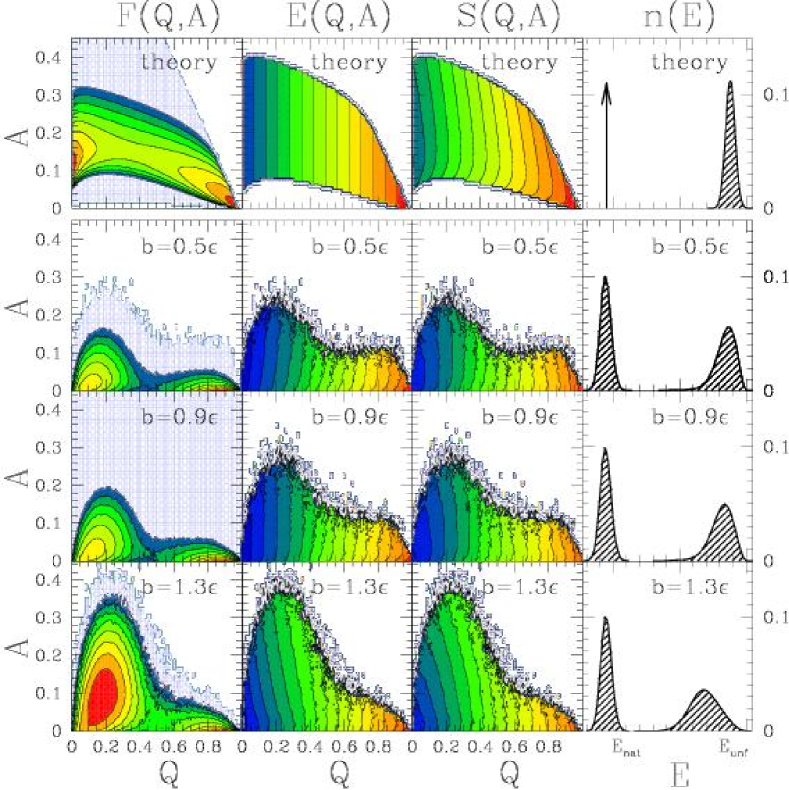
Figure 1:

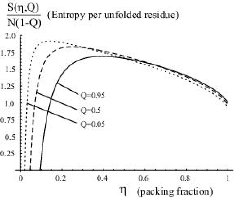
Figure 2:

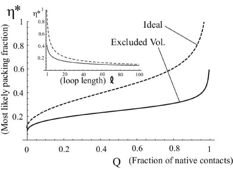
Figure 3:

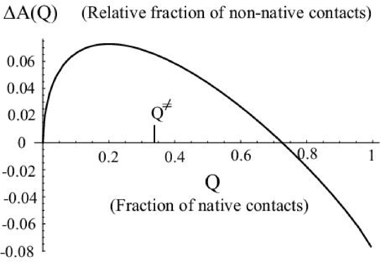
Figure 4:

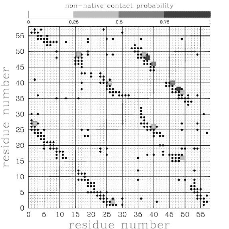
Figure 5:

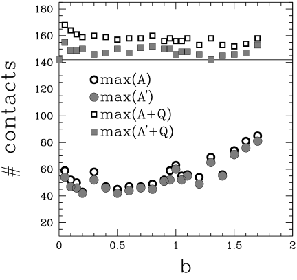
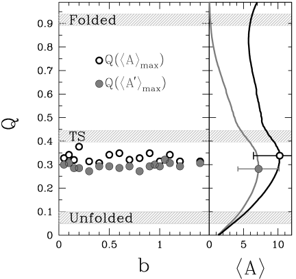
Figure 6:

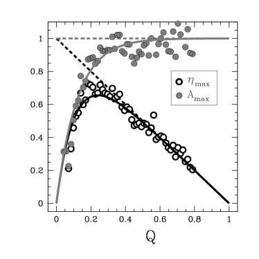
Figure 7:

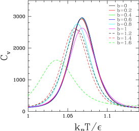
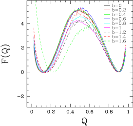
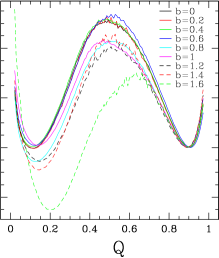
Figure 8:

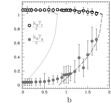
Figure 9:

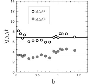
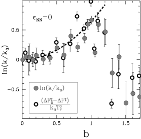
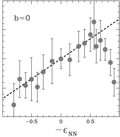
Figure 10:

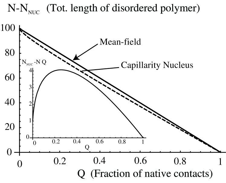
Figure 11:

Figure 12:

References

- (1) Winkler, J. R & Gray, H. R. (1998). Protein Folding. Accounts of Chemical Research 31, 798.
- (2) Fersht, A. L. (2000) Structure and Mechanism in Protein Science: A guide to Enzyme Catalysis and Protein Folding. (W.H. Freeman and Company, New York).
- (3) Creighton, T. E. (2002) Proteins: Structure and Molecular Properties. (W. H. Freeman and Company, New York).
- (4) Plotkin, S. S & Onuchic, J. N. (2002). Understanding Protein Folding with Energy Landscape Theory I: Basic Concepts. Quart. Rev. Biophys. 35, 111–167.
- (5) Plotkin, S. S & Onuchic, J. N. (2002). Understanding Protein Folding with Energy Landscape Theory II: Quantitative Aspects. Quart. Rev. Biophys. 35, 205–286.
- (6) Karanicolas, J & Brooks, C. (2003). The structural basis for biphasic kinetics in the folding of the WW domain from a formin-binding protein: Lessons for protein design? Proc. Natl. Acad. Sci. USA 100, 3954–3959.
- (7) Shea, J & Brooks III, C. (2001). From folding theories to folding proteins: A review and assessment of simulation studies of protein folding and unfolding. Ann. Rev. Phys. Chem. 52, 499–535.
- (8) Sorenson, J. M & Head-Gordon, T. (2000). Matching simulation and experiment: A new simplified model for simulating protein folding. J. Comput. Biol. 7, 469–481.
- (9) Shimada, J & Shakhnovich, E. (2002). The ensemble folding kinetics of protein G from an all-atom Monte Carlo simulation. Proc. Natl. Acad. Sci. USA 99, 11175–11180.
- (10) Shoemaker, B. A, Wang, J, & Wolynes, P. G. (1999). Exploring structures in protein folding funnels with free energy functionals: The transition state ensemble. J. Mol. Biol. 287, 675–694.
- (11) Clementi, C, Garcia, A. E, & Onuchic, J. N. (2003). Interplay among tertiary contacts, secondary structure formation and side-chain packing in the protein folding mechanism: an all-atom representation study. J. Mol. Biol. 326, 933–954.
- (12) Kaya, H & Chan, H. S. (2003). Solvation effects and driving forces for protein thermodynamic and kinetic cooperativity: How adequate is native-centric topological modeling? J. Mol. Biol. 326, 911–931.
- (13) Sorenson, J. M & Head-Gordon, T. (2002). Protein engineering study of protein L by simulation. J. Comput. Biol. 9, 35–54.
- (14) Ervin, J & Gruebele, M. (2002). Quantifying protein folding transition states with . J.Biol.Phys. 28, 115–128.
- (15) Lapidus, L. J, Eaton, W. A, & Hofrichter, J. (2000). Measuring the rate of intramolecular contact formation in polypeptides. Proc. Natl. Acad. Sci. U. S. A. 97, 7220–7225.
- (16) Schuler, B, Lipman, E. A, & Eaton, W. A. (2002). Probing the free-energy surface for protein folding with single-molecule fluorescence spectroscopy. Nature 419, 743–747.
- (17) Pande, V. (2003). Meeting halfway on the bridge between protein folding theory and experiment. Proc. Natl. Acad. Sci. USA 100, 3555–3556.
- (18) Snow, C, Nguyen, H, Pande, V, & Gruebele, M. (2002). Absolute comparison of simulated and experimental protein-folding dynamics. Nature 420, 102–106.
- (19) Kubelka, J, Eaton, W, & Hofrichter, J. (2003). Experimental tests of villin subdomain folding simulations. J. Mol. Biol. 329, 635–630.
- (20) Bryngelson, J. D, Onuchic, J. N, Socci, N. D, & Wolynes, P. G. (1995). Funnels, pathways and the energy landscape of protein folding. Proteins 21, 167–195.
- (21) Shoemaker, B. A, Wang, J, & Wolynes, P. G. (1997). Structural correlations in protein folding funnels. Proc. Nat. Acad. Sci. USA 94, 777–782.
- (22) Alm, E & Baker, D. (1999). Prediction of protein-folding mechanisms from free-energy landscapes derived from native structures. Proc Nat Acad Sci USA 96, 11305–11310.
- (23) Munoz, V & Eaton, W. A. (1999). A simple model for calculating the kinetics of protein folding from three-dimensional structures. Proc Nat Acad Sci USA 96, 11311–11316.
- (24) Galzitskaya, O. V & Finkelstein, A. V. (1999). A theoretical search for folding/unfolding nuclei in three dimensional protein structures. Proc Nat Acad Sci USA 96, 11299–11304.
- (25) Clementi, C, Jennings, P. A, & Onuchic, J. N. (2000). How native state topology affects the folding of Dihydrofolate Reductase and and Interleukin-1. Proc. Natl. Acad. Sci. USA 97, 5871–5876.
- (26) Clementi, C, Nymeyer, H, & Onuchic, J. N. (2000). Topological and energetic factors: what determines the structural details of the transition state ensemble and “en-route” intermediates for protein folding? An investigation for small globular proteins. J. Mol. Biol. 298, 937–953.
- (27) Shea, J. E, Onuchic, J. N, & Brooks, C. L. (2000). Energetic frustration and the nature of the transition state in protein folding. J Chem Phys 113, 7663–7671.
- (28) Clementi, C, Jennings, P. A, & Onuchic, J. N. (2001). Prediction of folding mechanism for circular-permuted proteins. J. Mol. Biol. 311, 879–890.
- (29) Plaxco, K. W, Larson, S, Ruczinski, I, Riddle, D. S, Thayer, E. C, Buchwitz, B, Davidson, A. R, & Baker, D. (2000). Evolutionary conservation in protein folding kinetics. J Mol Biol 298, 303–312.
- (30) Gunasekaran, K, Eysel, S, Hagler, A, & Gierash, L. (2001). Keeping it in the family: Folding studies of related proteins. Current Opinion in Structural Biology 11, 83–93.
- (31) Baker, D. (2000). A surprising simplicity to protein folding. Nature 405, 39–42.
- (32) Ferguson, N, Capaldi, A. P, James, R, Kleanthous, C, & Radford, S. E. (1999). Rapid folding with and without populated intermediates i the homologous four-helix porteins Im7 and Im9. J Mol Biol 286, 1597–1608.
- (33) Kim, D. E, Fisher, C, & Baker, D. (2000). A breakdown of symmetry in the folding transition state of protein L. J Mol Biol 298, 971–984.
- (34) Mines, G. A, Pascher, T, Lee, S. C, Winkler, J. R, & Gray, H. B. (1996). Cytochrome c folding triggered by electron transfer. Chem. and Biol. 3, 491–497.
- (35) Plaxco, K. W, Simons, K. T, Ruczinski, I, & Baker, D. (2000). Topology, stability, sequence, and length: Defining the determinants of two-state protein folding kinetics. Biochemistry 39, 11177–11183.
- (36) Ueda, Y, Taketomi, H, & Gō, N. (1975). Studies on protein folding, unfolding, and fluctuations by computer simulation. Int. J. Peptide Protein Res. 7, 445–459.
- (37) Fersht, A, Leatherbarrow, R, & Wells, T. (1986). Quantitative analysis of structural activity relationship in engineered proteins by linear free energy relationships. Nature 322, 284–286.
- (38) Matouschek, A, Kellis, J. T, Serrano, L, Bycroft, M, & Fersht, A. R. (1990). Transient folding intermediates characterized by protein engineering. Nature 346, 440–445.
- (39) Paci, E, Vendruscolo, M, & Karplus, M. (2002). Validity of Gō models: Comparison with a solvent-sheilded empirical energy decomposition. Biophys J 83, 3032–3038.
- (40) Plotkin, S. S. (2001). Speeding protein folding beyond the Gō model: How a little frustration sometimes helps. Proteins 45, 337–345.
- (41) Fan, K, Wang, J, & Wang, W. (2002). Folding of lattice protein chains with modified Gō potential. Eur Phys J B 30, 381–391.
- (42) Cieplak, M & Hoang, T. X. (2002). The range of the contact interactions and the kinetics of the Gō models of proteins. Int. J. Mod. Phys. C 13, 1231–1242.
- (43) Li, L, Mirny, L. A, & Shakhnovich, E. I. (2000). Kinetics, thermodynamics and evolution of non-native interactions in a protein folding nucleus. Nature Struct Biol 7, 336–342.
- (44) Treptow, W. L, Barbosa, M. A. A, Barcia, L. G, & de Araújo, A. F. P. (2002). Non-native Interactions, Effective Contact Order, and protein folding: A mutational investigation with the energetically frustrated hydrophobic model. Proteins 49, 167–180.
- (45) Sabelko, J, Ervin, J, & Gruebele, M. (1999). Observation of strange kinetics in protein folding. Proc. Natl. Acad. Sci. USA 96, 6031–6036.
- (46) Gruebele, M. (1999). The fast protein folding problem. Annu Rev Phys Chem 50, 485–516.
- (47) Viguera, A. R, Vega, C, & Serrano, L. (2002). Unspecific hydrophobic stabilization of folding transition states. Proc Nat Acad Sci USA 99, 5349–5354.
- (48) Honeycutt, J & Thirumalai, D. (1992). The nature of the folded state of globular proteins. Biopolymers 32, 695–709.
- (49) Plotkin, S. S & Clementi, C. (2003) The effect of non-native interactions on protein folding mechanism.
- (50) Goldstein, R. A, Luthey-Schulten, Z. A, & Wolynes, P. G. (1992). Optimal protein-folding codes from spin-glass theory. Proc Nat Acad Sci USA 89, 4918–4922.
- (51) Klimov, D & Thirumalai, D. (1996). Criterion that determines the foldability of Proteins. Phys Rev Lett 76, 4070–4073.
- (52) Wang, J, Plotkin, S. S, & Wolynes, P. G. (1997). Configurational diffusion on a locally connected correlated energy landscape; application to finite, random heteropolymers. J. Phys. I France 7, 395–421.
- (53) Takada, S, Portman, J. J, & Wolynes, P. G. (1997). An elementary mode coupling theory of random heteropolymer dynamics. Proc Nat Acad Sci USA 94, 23188–2321.
- (54) Eastwood, M. P & Wolynes, P. G. (2001). Role of explicitly cooperative interactions in protein folding funnels: a simulation study. Proteins 30, 215–227.
- (55) Derrida, B. (1981). Random-energy model: an exactly solvable model of disordered systems. Phys. Rev. B 24, 2613–26.
- (56) Bryngelson, J. D & Wolynes, P. G. (1987). Spin glasses and the statistical mechanics of protein folding. Proc Nat Acad Sci USA 84, 7524–7528.
- (57) Nymeyer, H, Socci, N. D, & Onuchic, J. N. (2000). Landscape approaches for determining the ensemble of folding transition states: Success and failure hinge on the degree of minimal frustration. Proc Nat Acad Sci USA 97, 634–639.
- (58) Klein-Seetharaman, J, Oikawa, M, Grimshaw, S. B, Wirmer, J, Duchardt, E, Ueda, T, Imoto, T, Smith, L. J, Dobson, C. M, & Schwalbe, H. (2002). Long-range interactions within a nonnative protein. Science 295, 1719–1722.
- (59) Zagrovic, B, Snow, C. D, Shirts, M. R, & Pande, V. S. (2002). Simulation of folding of a small alpha-helical protein in atomistic detail using worldwide-distributed computing. J. Mol. Biol. 323, 927–937.
- (60) Plotkin, S. S & Wolynes, P. G. (2003). Buffed energy landscapes: Another solution to the kinetic paradoxes of protein folding. Proc. Natl. Acad. Sci. USA 100, 4417–4422.
- (61) Plaxco, K. W, Simons, K. T, & Baker, D. (1998). Contact order, transition state placement and the refolding rates of single domain proteins. J Mol Biol 277, 985–994.
- (62) Flory, P. J. (1953) Principles of Polymer Chemistry. (Cornell University, Ithaca).
- (63) Sanchez, I. C. (1979). Phase transition behavior of the isolated polymer chain. Macromolecules 12, 980–988.
- (64) (1976). Symposium on the Amorphous State, J. Macromol. Sci. B12 (1,2).
- (65) Finkelstein, A. V & Badretdinov, A. Y. (1997). Rate of protein folding near the point of thermodynamic equilibrium between the coil and the most stable chain fold. Folding & Design 2, 115–121.
- (66) Ueda, Y, Taketomi, H, & Gō, N. (1975). Studies on protein folding, unfolding and fluctuations by computer simulation. I. The effects of specific amino acid sequence represented by specific inter-unit interactions. Int. J. Peptide Res. 7, 445–459.
- (67) Sobolev, V, Wade, R, Vriend, G, & Edelman, M. (1996). Molecular docking using surface complementarity. Proteins 25, 120–129.
- (68) Onuchic, J. N, Nymeyer, H, García, A. E, Chahine, J, & Socci, N. D. (1999). The Energy Landscape Theory of Protein Folding: Insights into Folding Mechanisms and Scenarios. Adv. Protein Chem. in press.
- (69) Pearlman, D. A, Case, D. A, Caldwell, J. W, Ross, W. S, Cheatam, T. E, Ferguson, D. M, Singh, U. C, Weiner, P, & Kollman, P. A. (1995) AMBER, V. 4.1.
- (70) Berendsen, H. J. C, Postma, J. P. M, van Gunsteren, W. F, DiNola, A, & Haak, J. R. (1984). Molecular dynamics with coupling to an external bath. J. Chem. Phys. 81, 3684–3690.
- (71) Ferrenberg, A. M & Swendsen, R. H. (1988). New Monte Carlo Technique for Studying Phase Transitions. Phys. Rev. Lett. 61, 2635–2638.
- (72) Ferrenberg, A. M & Swendsen, R. H. (1989). Optimaized Monte Carlo Data Analysis. Phys. Rev. Lett. 63, 1195–1198.