Maximum principle and mutation thresholds for four-letter sequence evolution

Abstract

A four-state mutation–selection model for the evolution of populations of DNA-sequences is investigated with particular interest in the phenomenon of error thresholds. The mutation model considered is the Kimura 3ST mutation scheme, fitness functions, which determine the selection process, come from the permutation-invariant class. Error thresholds can be found for various fitness functions, the phase diagrams are more interesting than for equivalent two-state models. Results for (small) finite sequence lengths are compared with those for infinite sequence length, obtained via a maximum principle that is equivalent to the principle of minimal free energy in physics.

1 Introduction

In population genetics, one aims to model the evolution of a population, taking into account evolutionary forces such as mutation, selection, recombination, or migration, using either a stochastic formulation, to incorporate the effects of a finite population, or a deterministic formulation, to emulate the limit of infinite population size. For a review, see [3].

In this paper, we are concerned with a deterministic mutation–selection model for a haploid population (or a diploid population without dominance). These types of models have been subject to investigation in various different settings, see [4]. The questions one is typically interested in comprise mutation–selection balance, mean quantities and variances, and the mutation load, i. e., the dependence of the mean fitness on the mutation rates.

One class of mutation–selection models are sequence space models, where, inspired by the structure of the DNA, genotypes are modelled as sequences written in a two- or four-letter alphabet, where each letter stands for one of the purines adenine and guanine, or the pyrimidines cytosine and thymine (or uracil in the case of RNA sequences). The majority of work in this field is done for two-state models, where one state is identified with purines and the other with pyrimidines, or, alternatively, one stands for a wildtype and the other for a mutant site; results for models that incorporate the full for-letter structure of the DNA are scarce [12, 10].

The advantage of sequence space models is that the mutation process is straightforward to model. A drawback is, however, that the modelling of the selection process is less clear. Selection comes in as different reproduction rates that are assigned to different genotypes. In nature, these are influenced by the phenotype, and the mapping from genotypes to phenotypes is highly complex, such that any feasible modelling of selection is necessarily simplistic.

Due to the linear structure and limited alphabet of the DNA, sequence space models are very similar to some physical models, such as one-dimensional Ising models or quantum spin chains. In fact, in an appropriate formulation, they are equivalent to these [19, 2]. The realization of this equivalence made the well developed methods and tools from statistical physics accessible in the population genetics context. The analogies between the physical and the biological models are however involved, as the observables and quantities of interest are slightly different in the different disciplines. One example for the transfer of knowledge from physics to biology is the derivation of a maximum principle for the population mean fitness, that finds its analog in physics in the principle of minimal free energy. This has been shown for a two-state model in [11], generalised to a four-state model in [10], and derived for a very general class of evolution models in biology in [1].

Of particular interest is the phenomenon of a mutation driven error threshold. This phenomenon is based on the antagonistic action of mutation and selection. For low mutation rates, selection dominates the population, such that its distribution is going to be clustered around the optimal sequence and thus is well localized in sequence space. At high mutation rates, on the other hand, mutation outweighs the effect of selection and the population distribution is an equidistribution in sequence space, which certainly leads to extinction. If the transition from the localised to the delocalized population distribution is very sharp and occurs in a very narrow regime of mutation rates, one speaks of an error threshold. This phenomenon is equivalent to phase transitions in physics, where the temperature takes the role of the mutation rate.

The existence of error thresholds in biology has been predicted in the framework of the quasi-species model [9], and attracted considerable interest ever since [20, 24, 21, 8, 11]. More recently, experimental indications for the existence of error thresholds in virus population have been reported, see for instance [7, 6].

Existence and properties of the error thresholds depend on the model of selection. Most theoretical investigations of the error threshold phenomenon are done for two-state models, the only work considering four-state models we are aware of is [12], and this is limited to a single fitness function. The results indicate however more involved phase diagrams than in the two-state case, warranting further investigations.

The scope of this work is to investigate a four-state mutation–selection model with particular attention for the phase diagrams with a number of different fitness functions using the maximum principle for the population mean fitness from [10] to determine the error thresholds.

The outline of the paper is as follows. In section 2, the general setup of our deterministic mutation–selection model is stated, introducing the quantities of interest. This is applied to the case of a four-state sequence space model in section 3. Section 4 introduces the major simplification of a permutation invariant fitness and presents the resulting reduction of the type space. In section 5, we recall the maximum principle from [10], which is applied to the investigation of error thresholds in section 6. Finally, we close with our conclusions.

2 Mutation selection models

The mathematical setup of a deterministic mutation–selection model for a haploid population (or a diploid one without dominance) in time-continuous formulation is as follows. Individuals are identified with genotypes, i. e., their fitness (or reproduction rate) is solely determined by the genotype and thus environmental effects are neglected. The number of genotypes is finite. In the case of sequences of a fixed length $N$ written in a four-letter alphabet, there are $4^{N}$ different sequences and thus genotypes. The set of genotypes forms the the type space $\mathfrak{S}$, which is also called sequence space in case of sequences as genotypes.

2.1 Population

The population at any time $t$ is described by the frequencies $p_{i}$ of each type $i\in\mathfrak{S}$, which are collected in the $|\mathfrak{S}|$-dimensional vector $\bi{p}(t)$, where $|\mathfrak{S}|$ is the cardinality of the type space. The population is a probability distribution and normalized such that $\sum_{i}p_{i}=1$.

2.2 Evolution of the population

Evolution is modelled in a time-continuous formulation. Mutation and selection are treated as two independent processes going on in parallel. In this case, the possible events are birth and death events for each type $i$, and mutation events from type $j$ to $i$, which happen with rates $b_{i}$, $d_{i}$ and $m_{ij}$, respectively. The effective reproduction rate is given by the difference of birth and death rates, $r_{i}=b_{i}-d_{i}$. The reproduction rates are collected in the diagonal reproduction matrix $\mathcal{R}=(r_{i})$. Similarly, the mutation rates are the entries of the mutation matrix $\mathcal{M}=(m_{ij})$. The diagonal entries of the mutation matrix are chosen such that $\mathcal{M}$ is a Markov generator and fulfils the condition $\sum_{i}\mathcal{M}_{ij}=0$. The time evolution operator $\mathcal{H}$ is given as the sum of reproduction and mutation matrix $\mathcal{H=R+M}$.

The evolution of the population is then given by the evolution equation

$$\dot{\bi{p}}(t)=\left[\mathcal{H}-\bar{r}(t)\mathbf{1}\right]\bi{p}(t)\;,$$ (1)

where $\bar{r}(t)=\sum_{i}r_{i}p_{i}(t)$ is the population mean fitness, and $\mathbf{1}$ is the unity matrix.

In equilibrium, $\dot{\bi{p}}=0$, thus this equation reduces to an eigenvalue equation of $\mathcal{H}$. All equilibrium quantities shall be denoted by omitting the argument $t$. So $\bar{r}$ is the population mean fitness in equilibrium for instance. Assuming irreducibility for $\mathcal{M}$, Perron-Frobenius theory [14] applies, which implies that the leading eigenvalue $\bar{r}$ is non-degenerate, and the corresponding (right) eigenvector $\bi{p}$ is strictly positive, as required for a probability distribution.

2.3 Relative reproductive success and ancestral distribution

Similarly to the population distribution, there is another distribution that will prove important in this model, namely the ancestral distribution.

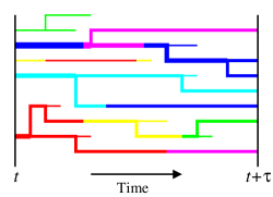
Figure 1: Schematic population: lineages symbolize individuals, colours indicate their types. Colour changes mark mutation events, whereas branching lines represent births and ending lines stand for deaths. The thickness of a line at any time denotes the number of offspring of the individual at time $t+\tau$.

Figure 1 shows schematically a population evolving in time in terms of a multitype branching process. The population distribution of this population at any time (between $t$ and $t+\tau$) is easily accessible by counting the number of lines of each type (colour) at that time and normalizing it.

The relative reproductive success $z_{i}(\tau,t)$ of type $i$ at time $t$ with respect to $t+\tau$ is proportional to the number of offspring at time $t+\tau$ of all individuals of type $i$ at time $t$ divided by the number of type $i$ individuals at time $t$. As shown in [11], for infinite populations in equilibrium ($t,\tau\rightarrow\infty$), the relative reproductive success $\bi{z}$ is given by the left Perron-Frobenius eigenvector of $\mathcal{H}$.

The ancestral distribution $\bi{a}(\tau,t)$ is derived by tracing back each line from $t+\tau$ to $t$ and counting it as the type it is at $t$, irrespective of its type at $t+\tau$. As this is a probability distribution, it has to be normalized such that $\sum_{i}a_{i}(\tau,t)=1$. Thus we get $a_{i}(\tau,t)=z_{i}(\tau,t)p_{i}(t)$, with a suitable normalization of $\bi{z}$, cf. [11], such that in equilibrium the $a_{i}$ are given by both the left and right PF-eigenvectors, $\bi{z}$ and $\bi{p}$.

2.4 Ancestral and population averages

Every quantity, say $f$, that is assigned to each type $i\in\mathfrak{S}$ can be averaged with respect to both the ancestral and population distribution. The population mean of $f$ is defined as

$$\bar{f}(t):=\sum_{i}f_{i}p_{i}(t)\;,$$ (2)

the population mean fitness from equation (1) is an important example. The ancestral mean of $f$ is given by

$$\hat{f}(\tau,t):=\sum_{i}f_{i}a_{i}(\tau,t)\;.$$ (3)

3 The four-state model

When modelling DNA or RNA evolution, the genotypes become sequences, that are written in a four-letter alphabet $\Sigma$ (or binary sequences in a simplified version). Here, we restrict ourselves to sequences of fixed length $N$, and thus the sequence space $\mathfrak{S}_{N}$ is the set of all four-state sequences $s$ of length $N$, $\mathfrak{S}_{N}=\Sigma^{N}$ with $\Sigma=\{\tt A,G,C,T\}$ and $|\mathfrak{S}_{N}|=4^{N}$.

3.1 Mutation model

The only mutation process taken into account is that of single point mutations, disregarding more complex events such as multiple mutations, deletions or insertions. This is known as the single step mutation model [22]. Site independent mutation rates are assumed. With four different nucleotides, there are 12 different replacements of one by another. The rates for these are specified by the Kimura 3ST mutation scheme [17, 23], cf. Figure 2, which uses only 3 different mutation rates, $\mu_{1},\mu_{2}$ and $\mu_{3}$.

Figure 2: Kimura 3ST mutation scheme.

Common simplifications of this model are the Jukes-Cantor mutation scheme [13], where all three mutation rates are the same, $\mu_{k}:=\mu$, $k=1,2,3$ and the Kimura 2 parameter model [16], where $\mu_{1}\equiv\mu_{3}:=\mu$, which takes into account only the different mutation rates for transitions, which are replacements of one of the purines (A or G) by the other, or of one of the pyrimidines (C or T) by the other, and transversions, which are replacements of a purine by a pyrimidine and vice versa. This is justified by the observation that transitions, which occur at rate $\mu_{2}$, are found to have a far higher rate than the two types of transversions, which happen at similar rates $\mu_{1}$ and $\mu_{3}$.

A convenient measure for closeness of two sequences is the Hamming distance $d_{H}$ [25], which counts the number of sites at which two sequences $s,s^{\prime}$ differ. In the single step mutation model, this determines how many mutational steps away from each other the two sequences are. Using the Kimura 3ST mutation scheme, one needs a 3-dimensional Hamming distance $\bi{d}_{H}(s,s^{\prime})$, to account for the different types of mutations. The $k$-th entry of the Hamming distance, $d_{H,\,k}$ simply counts the number of sites at which the sequences $s$ and $s^{\prime}$ differ in a way such that they can mutate into each other with rate $\mu_{k}$.

The entries of the mutation matrix are given by

$$\mathcal{M}_{s,s^{\prime}}=\cases{\mu_{1}/N&for $\bi{d}_{H}(s,s^{\prime})=(1,0,0)^{T}$\\ \mu_{2}/N&for $\bi{d}_{H}(s,s^{\prime})=(0,1,0)^{T}$\\ \mu_{3}/N&for $\bi{d}_{H}(s,s^{\prime})=(0,0,1)^{T}$\\ -(\mu_{1}+\mu_{2}+\mu_{3})&for $s=s^{\prime}$\\ 0&else \quad.}$$ (4)

3.2 Representation of sequences

Defining a reference type, which is usually (but not necessarily) taken to be the wildtype, i. e., the type with maximal fitness, we can conveniently change the alphabet $\Sigma$ from $\{{\tt A,G,C,T}\}$ to $\{0,1,2,3\}$. This is done by assigning the zero string to the reference type, $s_{\rm ref}=00\ldots 0$. The representation of any other sequence is obtained relative to the reference type. Comparing a sequence $s$ with the wildtype $s_{\rm ref}$, we assign $0$ to $s$ at each site where the two sequences match; at sites where they differ, we assign $1$, $2$ or $3$, depending on the type of mutation (determined by the respective mutation rate).

Using this representation we can define the mutational distance $\bi{d}$ as the 3-dimensional Hamming distance to the wildtype,

$$\bi{d}=\left(\begin{array}[]{c}d_{1}\\ d_{2}\\ d_{3}\end{array}\right)=\left(\begin{array}[]{c}\#1\\ \#2\\ \#3\end{array}\right)$$ (5)

with $0\leq d_{1},d_{2},d_{3}$ and the total mutational distance $d=\sum_{k=1}^{3}d_{k}\leq N$. The number of wildtype sites is given by $d_{0}=N-\sum_{k=1}^{3}d_{k}$. The mutational distance determines how many mutational steps of each type a sequence is away from the wildtype.

4 Permutation invariant fitness model

Whereas the mutation model is well justified on the microscopic level, the picture is different for the reproduction rates. Only little is known about the nature of realistic fitness functions, and any realistic fitness function would be highly complex and probably too hard to tackle analytically. Usually, the choice of fitness function is determined rather by feasibility than by closeness to reality.

One rather common, though often implicitly used, assumption is that of a permutation-invariant fitness function. This means that the reproduction rate of a sequence depends only on its mutational distance to the wildtype, not on the order of the sequence and implies that all sequences with the same mutational distance have the same fitness.

Of course this assumption is highly unrealistic, as in nature the location of a mutation (whether it lies in a coding or non-coding region of the genome, for instance) will certainly influence the fitness. Having said that, the accumulation of many mutations with small effects on the fitness is described surprisingly well by a permutation-invariant fitness. In contrast to, for instance, magnetic systems in physics, where the interactions are rather short ranged, and therefore next-neighbour interactions seem more appropriate than permutation-invariant ones, in the genome the interactions are typically long-ranged, and therefore the permutation-invariant fitness is a natural choice.

For a permutation-invariant fitness, we can reduce the dimensions of the type space by a procedure that is known as lumping in the theory of Markov chains ([15], Chapter VI). The essence here is that multiple classes are lumped together in one class, such that a new Markov process with fewer classes emerges. In our case we want to lump together all sequences with the same fitness, such that the lumped types are determined by the mutational distance $\bi{d}$. This implies that the lumping is compatible with the mutation scheme, which imposes the structure on the type space.

4.1 The mutational distance space

The sequence space $\mathfrak{S}$ contains all $\{0,1,2,3\}$-sequences $s$ of length $N$, $\mathfrak{S}=\Sigma^{N}$, and thus $|\mathfrak{S}|=4^{N}$. The neighbourhood or structure of this space is determined by the mutation model: Two sequences are neighbours if and only if they can mutate into one another with a single mutational step, i. e.  they differ only at a single site. Thus each sequence has $3N$ neighbours as there are N sites and three types of mutation at each site.

The lumped type space, or mutational distance space $\mathcal{S}$ contains the $(N+1)(N+2)(N+3)/6$ different mutational distances $\bi{d}$. Going from the original sequence space $\mathfrak{S}$ to the mutational distance space $\mathcal{S}$, the neighbourhood is maintained, i. e., those and only those sequences $s^{\prime}$ that are neighbours of a particular sequence $s$ are in classes $\bi{d}^{\prime}$ that are neighbours of $\bi{d}$, the mutational distance of $s$. As $\mathcal{S}$ contains all possible mutational distances $\bi{d}$, it can be visualized as a simplex in $\mathbb{N}^{3}$.

Describing the neighbourhood of the mutational distances, it is useful to classify the sites of a sequence into wildtype and mutant sites, where the wildtype sites are those denominated by $0$, whereas the mutant sites are the $1,2,3$-sites. A mutation at a wildtype site changes this site to a mutant site and thus increases the total mutational distance $d$ to $d^{\prime}=d+1$. This is symbolised by

$$\bi{d}\rightarrow\bi{d}^{\prime}=\bi{d}+\bi{e}_{k}\quad\mbox{with}\quad\bi{e}_{k}=\cases{(1,0,0)^{T}&for $k=1$\\ (0,1,0)^{T}&for $k=2$\\ (0,0,1)^{T}&for $k=3$ \;.}$$ (6)

These mutations occur at rate $\mu_{k}d_{0}/N$.

For a mutation at a mutant site, there are two possibilities. Firstly, it can be a mutation from type $k$ back to the wildtype with rate $\mu_{k}$ and thus decrease the total mutational distance; in this case the mutational direction is given by $-\bi{e}_{k}$ with the $\bi{e}_{k}$ from equation (6). Secondly, it can be a mutation to another type of mutant site, which does not change the total mutational distance $d$, but changes the components of the mutational distance $\bi{d}$ to $\bi{d}^{\prime}=\bi{d}\pm\bi{e}_{+k,-\ell}$ with

$$\bi{e}_{+k,-\ell}=\cases{(1,-1,0)^{T}&for $k=1,\ell=2$\\ (1,0,-1)^{T}&for $k=1,\ell=3$\\ (0,1,-1)^{T}&for $k=2,\ell=3$}\;.$$ (7)

These mutations happen at rate $\mu_{m}d_{\ell}/N$ and $\mu_{m}d_{k}/N$, with $\{k,\ell,m\}=\{1,2,3\}$, respectively.

4.2 The lumped reproduction and mutation matrices

As we assume that fitness is permutation invariant and we lump together all sequences with the same mutational distance, the lumped reproduction matrix $\bi{R}$ is diagonal, too, and it is easily obtained as $\bi{R}_{\bi{d}}=\mathcal{R}_{s}$ with $\bi{d}=\bi{d}(s)$.

The lumped mutation matrix $\bi{M}$ differs more from the original $\mathcal{M}$. The only nonzero entries (apart from the diagonal) are the mutation rates between neighbouring mutational distances. They are given by

$$\eqalign{\bi{d}\rightarrow\bi{d}+\bi{e}_{k}:&\bi{M}_{\bi{d}+\bi{e}_{k},\bi{d}}=\mu_{k}d_{0}/N\\ \bi{d}\rightarrow\bi{d}-\bi{e}_{k}:&\bi{M}_{\bi{d}-\bi{e}_{k},\bi{d}}=\mu_{k}d_{k}/N\\ \bi{d}\rightarrow\bi{d}+\bi{e}_{k}-\bi{e}_{\ell}:&\bi{M}_{\bi{d}+\bi{e}_{k}-\bi{e}_{\ell},\bi{d}}=\mu_{m}d_{\ell}/N}$$ (8)

with $\{k,\ell,m\}=\{1,2,3\}$, taking into account the number of different sites at which the mutation can take place with the same effect. Using the same diagonal entries as in $\mathcal{M}$, i. e., $M_{\bi{d,d}}=-\sum_{k}\mu_{k}$, the mutation matrix is still a Markov generator. Note that $\bi{M}$ is, however, not symmetric in contrast to $\mathcal{M}$. For details of the lumping procedure, see [15, 10].

The lumped time evolution operator $\bi{H}$ is as before given as the sum of reproduction and mutation matrix, $\bi{H}=\bi{R+M}$. In the lumped system, the evolution equation takes the same form as before (see equation (1)).

4.3 Reversibility of $\bi{M}$

The equilibrium distribution (or PF-eigenvector) $\bi{\pi}$ of $\bi{M}$ is given by the number of sequences lumped into each mutational distance,

$$\pi{d}={N\choose d_{0},d_{1},d_{2},d_{3}}=\frac{N!}{d_{0}!d_{1}!d_{2}!d_{3}!}\;.$$ (9)

Thus $\pi_{\bi{d+e}_{k}}=\pi{d}\,d_{0}/(d_{k}+1)$ and similarly for other mutational steps. Using this, it can easily be verified that $\bi{M}$ is reversible (i. e., the detailed balance holds),

$$\bi{M_{d,d^{\prime}}\pi_{d^{\prime}}=M_{d^{\prime},d}\pi_{d}}\;,$$ (10)

and as $\bi{R}$ is diagonal, this holds likewise for $\bi{H}$: $\bi{H_{d,d^{\prime}}\pi_{d^{\prime}}=H_{d^{\prime},d}\pi_{d}}$.

5 Maximum principle

One of the quantities of main interest is the population mean fitness in equilibrium, $\bar{r}$, which is given by the leading eigenvalue of $\bi{H}$. In principle, this can be obtained by Rayleigh’s variational principle. Here, this is however not useful, as the optimization would have to be carried out over a space of dimension $(N+1)(N+2)(N+3)/6$. Using the assumption of a permutation-invariant fitness and the lumped Markov chain, Rayleigh’s principle can be reduced to an optimization over a single scalar in the case of binary sequences [11], or over the three components of the mutational distance our case of four-state sequences [10]. A general reduction of Rayleigh’s principle is derived in [1]. Here, we shall briefly repeat the derivation of the maximum principle.

5.1 Symmetrization of $\bi{H}$

Due to the reversibility of $\bi{M}$, the time-evolution operator $\bi{H}$ can be symmetrized by the means of a diagonal transformation,

$$\widetilde{\bi{H}}=\bi{\Pi}^{-1/2}\bi{H\Pi}^{1/2}$$ (11)

using the mutational equilibrium $\bi{\Pi}={\rm diag}\{\pi_{\bi{d}}\}$. $\widetilde{\bi{H}}$ has the same spectrum as $\bi{H}$.

The off-diagonal entries of $\widetilde{\bi{H}}$ are given by the symmetrized mutation rates $\widetilde{\bi{H}}_{\bi{d,d^{\prime}}}=\widetilde{\bi{M}}_{\bi{d,d^{\prime}}}=\bi{M_{d,d^{\prime}}}\sqrt{\frac{\pi{d^{\prime}}}{\pi_{\bi{d}}}}=\sqrt{\bi{M_{d,d^{\prime}}M_{d^{\prime},d}}}$. The symmetrized mutation rates are thus explicitly given by

$$\eqalign{\bi{d}\rightarrow\bi{d}+\bi{e}_{k}:&\widetilde{\bi{M}}_{\bi{d}+\bi{e}_{k},\bi{d}}=\frac{\mu_{k}}{N}\sqrt{d_{0}(d_{k}+1)}\\ \bi{d}\rightarrow\bi{d}-\bi{e}_{k}:&\widetilde{\bi{M}}_{\bi{d}-\bi{e}_{k},\bi{d}}=\frac{\mu_{k}}{N}\sqrt{d_{k}(d_{0}+1)}\\ \bi{d}\rightarrow\bi{d}+\bi{e}_{k}-\bi{e}_{\ell}:&\widetilde{\bi{M}}_{\bi{d}+\bi{e}_{k}-\bi{e}_{\ell},\bi{d}}=\frac{\mu_{m}}{N}\sqrt{d_{\ell}(d_{k}+1)}\;.}$$ (12)

The diagonal entries of $\bi{H}$ are unchanged by this transformation.

5.2 Splitting up $\widetilde{\bi{H}}$

The next step is to split up the symmetrized time-evolution operator $\widetilde{\bi{H}}$ into the sum of a Markov generator and a diagonal matrix that contains the remainder,

$$\widetilde{\bi{H}}=\bi{E+F}$$ (13)

with $\bi{F}$ being the (symmetric) Markov generator and $\bi{E}$ being the (diagonal) remainder. Clearly, the off-diagonal entries of $\bi{F}$ are given by the symmetrized mutation rates, $\bi{F_{d^{\prime},d}}=\widetilde{\bi{M}}_{\bi{d^{\prime},d}}$. For $\bi{F}$ to be a Markov generator, we need $\sum{d^{\prime}}\bi{F_{d^{\prime},d}}=0$, and hence the diagonal entries are given by

$$\eqalign{\bi{F_{d,d}}=-\sum_{\bi{d^{\prime}\neq d}}\bi{F_{d^{\prime},d}}=&-\sum_{k}\mu_{k}/N\left[\sqrt{d_{0}(d_{k}+1)}+\sqrt{d_{k}(d_{0}+1)}\right]\\ &-\sum_{k,\ell\atop k>\ell}\mu_{m}/N\left[\sqrt{d_{\ell}(d_{k}+1)}+\sqrt{d_{k}(d_{\ell}+1)}\right]\;,}$$ (14)

using the mutation rates (12). The entries of $\bi{E}$ are given by

$$\bi{E_{d}}=\bi{R_{d}}+\bi{M_{d,d}}-\bi{F_{d,d}}\;.$$ (15)

5.3 The maximum principle

In the limit $N\rightarrow\infty$ the matrices $\bi{E}$ and $\bi{F}$ can be approximated by functions $E$ and $F_{\xi}$

$$\bi{E_{d}}=E(\bi{x_{d}})+\Or\left(\frac{1}{N}\right)\quad\mbox{and}\quad\bi{F_{d^{\prime},d}}=F_{\pm\xi}(\bi{x_{d}})+\Or\left(\frac{1}{N}\right)\;,$$ (16)

where the $\bi{x_{d}}$ are normalized mutational distances $\bi{x_{d}}=\bi{d}/N$ with $0\leq x_{k}$, $\sum_{k=1}^{3}x_{k}\leq 1$ and the $\xi$ labels the possible directions of mutation $k$ or $+k,-\ell$ with $k,\ell\in\{1,2,3\}$ and $k>\ell$. $F_{\bi{d},\bi{d}^{\prime}}=0$ for non-neighbouring sequences $\bi{d},\bi{d}^{\prime}$.

Using the normalized mutational distances $\bi{x}$, we get also a normalized version of the mutational distance space, $\mathcal{S}\subset\mathbb{R}^{3}$, where the points become dense in the limit $N\rightarrow\infty$.

The $F_{\pm\xi}(\bi{x})$ are given approximately by the symmetrized mutation rates as

$$F_{\pm k}(\bi{x})\approx\mu_{k}\sqrt{x_{0}x_{k}}\;,\quad F_{\pm k\mp\ell}(\bi{x})\approx\mu_{m}\sqrt{x_{\ell}x_{k}}\;,$$ (17)

with the fraction of the wildtype sites $x_{0}=1-\sum_{k}x_{k}$ and $\{k,\ell,m\}=\{1,2,3\}$. For $E(\bi{x})$ we have

$$E(\bi{x})=r(\bi{x})-g(\bi{x})$$ (18)

with the fitness function $\bi{R_{d}}=r(\bi{x_{d}})+\Or({\textstyle\frac{1}{N}})$ and the mutational loss function

$$g(\bi{x}):=\sum_{k}\mu_{k}\left[1-2\sqrt{x_{0}x_{k}}-2\sum_{\ell,m\neq k\atop\ell>m}\sqrt{x_{\ell}x_{m}}\right]\;.$$ (19)

According to [1], Theorem 1, the population mean fitness in equilibrium is then given by the maximum principle

$$\bar{r}=\sup{x}\left[r(\bi{x})-g(\bi{x})\right]+\Or({\textstyle\frac{1}{N}})\;,$$ (20)

where the supremum is assumed at the ancestral mean mutational distance $\hat{\bi{x}}$, if $E(\bi{x})$ assumes its maximum in the interior of $\mathcal{S}$ (which is the generic case).

5.3.1 Validity.

The maximum principle is exact in the limit $N\rightarrow\infty$ as well as in the case of a linear fitness function $r(\bi{x})$ and for unidirectional mutation rates, which is not the case for our mutation model. For finite $N$ (and non-linear fitness function), it is correct up to $\Or\left({\textstyle\frac{1}{N}}\right)$ [1].

6 Mutation thresholds

6.1 The phenomenon

Analogously to the temperature-driven phase transition in physics, for certain choices of fitness functions one can observe the phenomenon that the order of the population breaks down at a critical mutation rate, and for any mutation rates higher than this, the population is delocalized in sequence space. In the population genetics context, this phenomenon is known as mutation-driven error threshold.

We define the phenomenon of the mutation threshold for systems with infinite sequence length $N\rightarrow\infty$ as a critical mutation rate $\bi{\mu}_{c}=(\mu_{1,c},\mu_{2,c},\mu_{3,c})$, at which there is a kink in the equilibrium population mean fitness $\bar{r}$ and a discontinuity in the ancestral mean mutational distance $\hat{\bi{x}}$, cf. the definition of the fitness-threshold in [11]. As this is a collective phenomenon, for finite sequence length, the transitions are smoothed out, and the critical mutation rates may be shifted a bit. Using the maximum principle (20), however, we can detect the discontinuities in $\hat{\bi{x}}$, as this is exact in the limit $N\rightarrow\infty$.

Figure 3 shows an example of an error threshold for the Kimura 2 parameter mutation model with $\mu=2\mu_{2}$ and a quadratic symmetric fitness

$$r(\bi{x})=-\sum_{k=1}^{3}x_{k}+\sum_{k,\ell=1\atop k\leq\ell}^{3}x_{k}x_{\ell}\;.$$ (21)

Figure 3: Example of a phase transition for Kimura 2 parameter mutation scheme with $\mu=2\mu_{2}$ and a quadratic symmetric fitness $r(\bi{x})=-\sum_{k}x_{k}+\sum_{k\leq\ell}x_{k}x_{\ell}$.

As the fitness function is symmetric with respect to the $x_{k}$, and the K2P mutation scheme breaks the symmetry only between $x_{2}$ vs. $x_{1},x_{3}$, in equilibrium we have $\hat{x}_{1}=\hat{x}_{3}$.

In Figure 3, one can see the decline in population mean fitness for mutation rates below the critical rate, which goes in line with an increase in ancestral mean mutational distance $\hat{\bi{x}}$. At the critical mutation rate, $\mu_{2,c}\approx 0.26$, the population mean fitness has a kink, and the ancestral mean mutational distance $\hat{\bi{x}}$ jumps to the completely random mutational distance with $\hat{x}_{0}=\hat{x}_{1}=\hat{x}_{2}=\hat{x}_{3}={\textstyle\frac{1}{4}}$, where it stays for all higher mutation rates, and consequently, the population mean fitness $\bar{r}$ stays constantly at its minimum value.

6.2 Choice of fitness functions

Error thresholds do not occur for all fitness functions, but only for some classes. For two-state models, there exist criteria for fitness functions to give rise to error thresholds [11]. For our four-state model, it is plausible to assume that the situation is similar.

It is easy to verify for the four-state model, that there can be no error thresholds for linear fitness functions. For a fitness function to give rise to error thresholds, one needs at least the complexity of a quadratic function. In the following, we will investigate two examples of fitness functions displaying error thresholds, namely a quadratic fitness function and a truncation selection, where all genotypes with less than a critical number of mutations are equally fit and all others equally unfit.

For simplicity, we will limit ourselves in our examples to the Kimura 2 parameter (K2P) and Jukes-Cantor (JC) mutation schemes as simplifications of the full Kimura 3ST mutation scheme, and restrict the choice of fitness functions to those that are symmetric with respect to the $x_{k}$, $k\in\{1,2,3\}$.

6.3 Quadratic symmetric fitness function

It can be shown that for quadratic fitness functions with positive epistasis, i. e., fitness functions with negative second derivatives, there exist no phase transitions (cf. [12]). Looking only at quadratic symmetric fitness functions with negative epistasis (or positive second derivative), a fairly general form is

$$r(\bi{x})=c\sum_{k=1}^{3}x_{k}+\sum_{k,\ell=1\atop k\leq\ell}^{3}x_{k}x_{\ell}\;.$$ (22)

Here, the parameter $c$ is used to tune the linear part relative to the quadratic term. The only possible generalization within our restricted setup would be to give different coefficients for the pure quadratic terms $x_{k}^{2}$ and the mixed quadratic terms $x_{k}x_{\ell}$ with $k\neq\ell$. We will however concentrate on the fitness given in equation (22).

In general, this fitness is symmetric with respect of the $x_{k}$, $k\in\{1,2,3\}$. For $c=-1$, the symmetry of the fitness function is even higher and includes the fraction of the wildtype-sites, $x_{0}=1-\sum_{k=1}^{3}x_{k}$. This is the fitness function that has been used for the example of an error threshold in Figure 3.

As the K2P mutation model has an inherent symmetry between $x_{1}$ and $x_{3}$, and between $x_{2}$ and $x_{0}$, respectively, and the fitness function (22) for arbitrary $c$ is symmetric with respect to the $x_{k}$, $k\in\{1,2,3\}$, it is evident that the equilibrium solution for the ancestral mean mutational distance mirrors that symmetry with $\hat{x}_{1}=\hat{x}_{3}$ (and in the case of $c=-1$, also $\hat{x}_{2}=\hat{x}_{0}$).

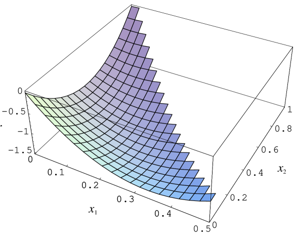
Figure 4: The quadratic symmetric fitness function (22) for $c=-1$ as a projection onto the relevant subspace with $x_{1}=x_{3}$.

Figure 4 shows the quadratic symmetric fitness function (22) for $c=-1$ as a projection onto the relevant subspace where $x_{1}=x_{3}$. The additional symmetry in the case $c=-1$ can be seen from the fact that there are two equally high maxima at $(x_{1},x_{2})=(0,0)$ and $(x_{1},x_{2})=(0,1)$.

6.3.1 Phase diagrams.

We have examined the phase diagrams for the K2P mutation model with the quadratic symmetric fitness function (22) for the possible combinations of mutation rates and the parameter $c$.

Figure 5: Phase diagram for the K2P mutation model and the quadratic symmetric fitness function (22) with $c=-1$. At the first order phase transition (solid line) the ancestral mean mutational distance $\hat{\bi{x}}$ jumps and the population mean fitness $\bar{r}$ has a kink, whereas at the second order phase transitions (dashed lines) this kink in $\bar{r}$ is reduced to a kink in its first derivative and the jump in $\hat{\bi{x}}$ is reduced to an infinite derivative at the critical mutation rate.

For the case $c=-1$, the phase diagram is shown in Figure 5, cf. [12], where a different notation, but the same fitness and mutation model are used. Here, we can identify 3 different phases:

• The AGCT phase. The population is essentially ordered, i. e., the population distribution is localized in sequence space.

• The disordered phase. The population is completely random, the population distribution is the equidistribution in sequence space, the ancestral mean mutational distance is given by $\hat{x}_{0}=\hat{x}_{1}=\hat{x}_{2}=\hat{x}_{3}={\textstyle\frac{1}{4}}$.

• The PP phase. A partially ordered phase, which only differentiates between purines and pyrimidines. In the ancestral distribution, there are two peaks that are equidistributions with respect to $x_{1},x_{3}$– and $x_{0},x_{2}$–direction, respectively, but localized in the other directions. This phase only exists in the case $c=-1$.

If the symmetry between $x_{0}$ and $x_{2}$ is broken, i. e., $c\neq-1$, the PP phase disappears, see Figures 6 and 7 for $c\leq-1$ and $c\geq-1$, respectively.

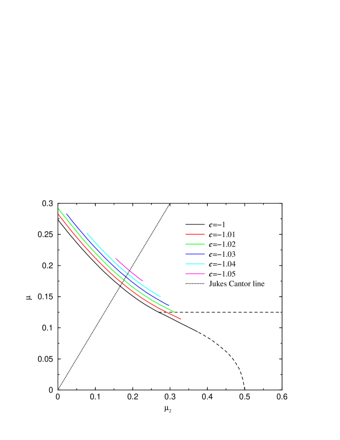
Figure 6: Phase diagram for the K2P mutation model and the quadratic symmetric fitness function (22) with $c\leq-1$.

For $c<-1$, cf. Figure 6, the second order phase transitions disappear immediately with the broken symmetry, the 1st order phase transition lines shrink with decreasing $c$ while shifting to slightly higher mutation rates and disappear for any $c\leq-1.06$. The disappearance of the 2nd order transitions implies a disappearance of the disordered and the PP phase, leaving only an AGCT phase with varying degrees of order.

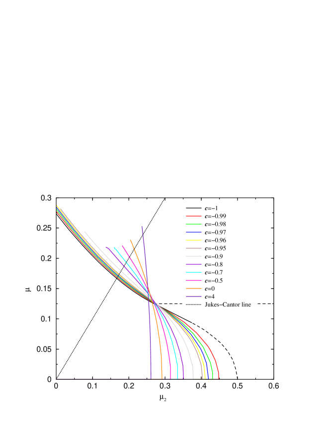
Figure 7: Phase diagram for the K2P mutation model and the quadratic symmetric fitness function (22) with $c>-1$.

In the case $c>-1$, cf. Figure 7, the PP phase merges with the disordered phase, such that only the AGCT and disordered phases remain. The second order phase transition between AGCT and PP phase in the case $c=-1$ is transformed to a first order transition.

6.3.2 Finite size effects.

Using the maximum principle (equation (20)), only the population mean fitness $\bar{r}$ and the ancestral mutational distance $\hat{\bi{x}}$ are accessible, which is sufficient to detect phase transitions. For small sequence length, it is however feasible to calculate $\bar{r}$ as largest eigenvalue and the population and ancestral distributions $\bi{p}$ and $\bi{a}$ through the corresponding eigenvector of $\widetilde{\bi{H}}$.

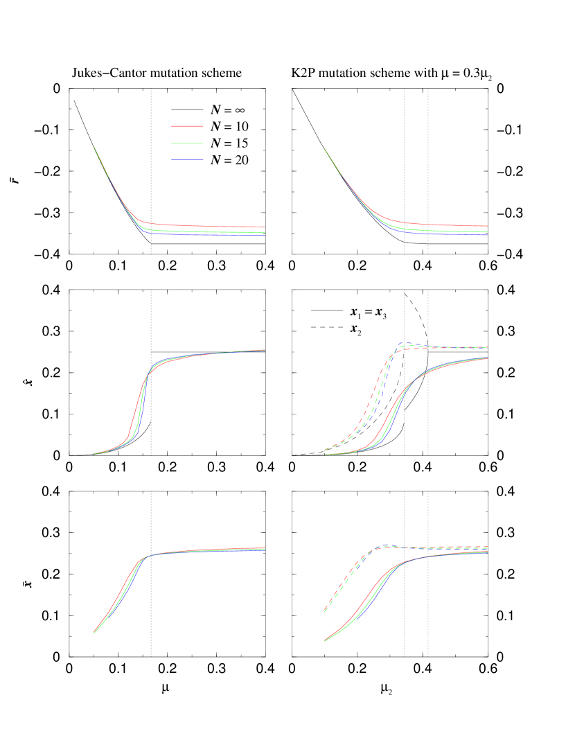
Figure 8: Comparison of population mean fitness $\bar{r}$, ancestral mean mutational distance $\hat{\bi{x}}$ and population mean mutational distance $\bar{\bi{x}}$ for different sequence length and the infinite system with fitness function (22) with $c=-1$. Left: JC mutation scheme, right: K2P mutation scheme with $\mu=0.3\mu_{2}$. The locations of the phase transitions are marked as vertical dotted lines.

Figure 8 shows results obtained this way for different finite sequence lengths using the quadratic fitness function (22) with parameter $c=-1$ compared with the results obtained via maximum principle (20), which are exact for an infinite system. On the left, the JC mutation model was used, and consequently, the mean mutational distances in all three directions coincide. On the right, the K2P mutation model with $\mu=0.3\mu_{2}$ was used. Here, the mean mutational distances in $x_{1}$ and $x_{3}$ direction coincide, but differ from those in $x_{2}$ direction.

In Figure 8 one can clearly see how the phase transitions, which are very sharp in the infinite system, are smoothed out for finite sequence length. Especially the second order phase transition in the K2P model cannot be detected at the sequence lengths considered here.

6.3.3 Distributions.

The results in Figure 8 have been obtained by calculating the population and ancestral distributions explicitly. Examples of these are visualized in Figures 9 to 11. Although for the mean mutational distance we have $x_{1}=x_{3}$ and therefore can reduce the sequence space to the 2-dimensional subspace, sequences with $x_{1}\neq x_{3}$ do occur in the equilibrium distributions with non-zero frequency, and thus we need the full three-dimensional mutational distance space $\mathcal{S}$ for the visualization. In Figures 9 to 11, the frequency of each point $\bi{d}$ is visualized as a cube of proportional size. For easier recognition, each cube corresponds to a block of 8 data points. The colours of the cubes indicate their position along the $x_{2}$ direction.

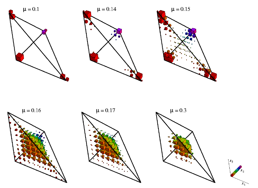
Figure 9: Ancestral distribution $\bi{a}$ for the JC mutation model with quadratic symmetric fitness (22) and $c=-1$ for selected mutation rates for a sequence length of $N=20$. The frequency of each type $\bi{d}$ is symbolized by a cube of proportional size. Colours indicate the position along the $x_{2}$ direction. For easier recognition, each cube corresponds to a block of 8 data points.

Figure 9 shows the ancestral distribution of the JC mutation model with the quadratic symmetric fitness function (22) with parameter $c=-1$. The phase transition, which happens around a mutation rate of $\mu\approx 0.16$, is clearly visible. For lower mutation rates, the population is in the AGCT phase and the ancestral distribution is localized. For mutation rates beyond the threshold, the population is in the disordered phase and the ancestral distribution is the equidistribution in sequence space. Note that the term equidistribution refers to the $4^{N}$-dimensional sequence space $\mathfrak{S}$, and thus we have a multinomial distribution in the depicted mutational distance space $\mathcal{S}$.

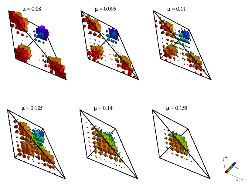
Figure 10: Population distribution $\bi{p}$ for the JC mutation model with fitness (22) and $c=-1$ for selected mutation rates for a sequence length of $N=20$. For easier recognition, each cube corresponds to a block of 8 data points.

In Figure 10, the population distributions for the same model and parameter values as in Figure 9 are shown. The population distribution goes through the same stages as the ancestral distribution, but at lower mutation rates, and in contrast to the ancestral distribution, the transition is smooth, as can be seen already in Figure 8.

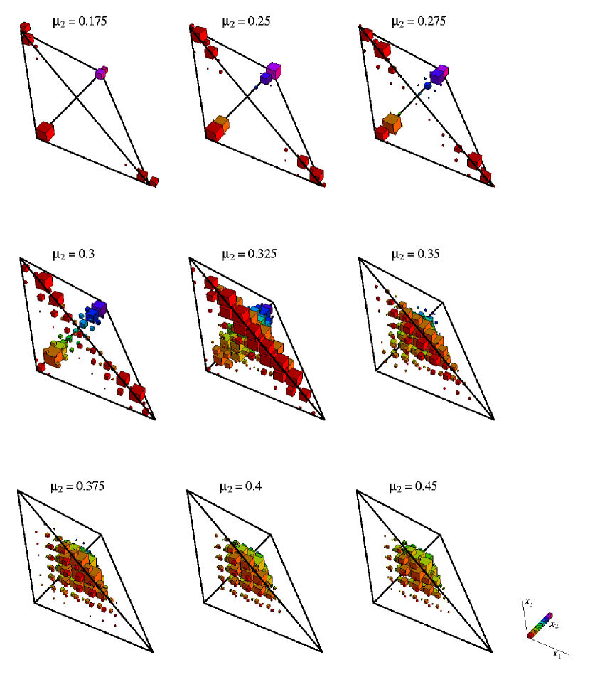
Figure 11: Ancestral distribution $\bi{a}$ for the K2P mutation model with $\mu=0.3\mu_{2}$ with fitness (22) and $c=-1$ for selected mutation rates for a sequence length of $N=20$. For easier recognition, each cube corresponds to a block of 8 data points.

Figure 11 shows the ancestral distribution for the K2P mutation model with $\mu=0.3\mu_{2}$ and fitness function (22) with $c=-1$. Here, the population starts in the AGCT phase (mutation rates $\mu_{2}<0.3$) and goes through the PP phase (at $\mu_{2}=0.325$), where the distribution constists of two “rods”, which are each an equidistribution with respect to the $x_{2},x_{0}$ or the $x_{3},x_{1}$ direction, respectively, and localized with respect to the remaininig directions. For high mutation rates, we find again the equidistribution of the disordered phase ($\mu_{2}>0.4$).

6.4 Truncation selection

Another fitness we are interested in is truncation selection, a case of extreme epistasis, both positive and negative. We use it in the form

$$r(\bi{x})=\left\{\begin{array}[]{cl}1&\mbox{if }\sum_{k}x_{k}\leq 3x_{c}\\[4.30554pt] 0&\mbox{if }\sum_{k}x_{k}>3x_{c}\quad.\end{array}\right.$$ (23)

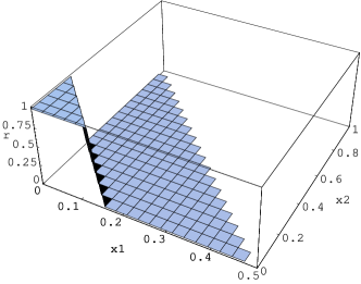
Figure 12: Truncation selection (23) for $x_{c}=0.1$ as a projection on the subspace $x_{1}=x_{3}$.

Figure 12 shows a projection of the truncation selelction (23) with $x_{c}=0.1$ onto the subspace $x_{1}=x_{3}$.

This is a generalization of the single-peaked landscape, where one single genotype is of high fitness and all others are equally unfit. The single peaked landscape has been widely used as an oversimplistic toy model. It has first been suggested in the context of prebiotic evolution [9] and corresponds to $x_{c}=0$ in our setting. Truncation selection with non-zero $x_{c}$, however, is a standard model in biology, e. g. [18].

6.4.1 Phase diagram.

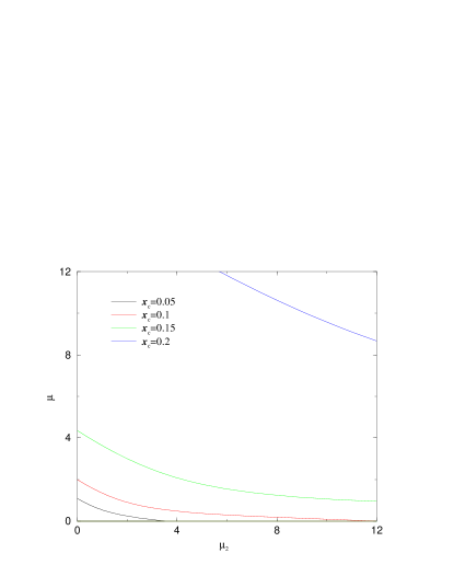
Figure 13: Left: Phase diagram for truncation selection (23) with different values of $x_{c}$. Right: Critical mutation rate $\mu_{c}$ against $x_{c}$ for truncation selection (23) and the JC mutation model.

On the left, Figure 13 shows the phase diagram for truncation selection (23) with different values of $x_{c}$. Here, we find error thresholds for all values of $x_{c}<{\textstyle\frac{1}{4}}$. For values of $x_{c}\geq{\textstyle\frac{1}{4}}$, the point of the mutation equilibrium, $\bi{x}=({\textstyle\frac{1}{4}},{\textstyle\frac{1}{4}},{\textstyle\frac{1}{4}})$, is included in the high plateau and thus the population will be in mutation equilibrium and at optimal fitness simultaneously for any mutation rate. On the right, Figure 13 shows the dependence of the critical mutation rate on $x_{c}$ in the JC mutation model. At $x_{c}={\textstyle\frac{1}{4}}$, the critical mutation rate diverges.

6.4.2 Finite size effects.

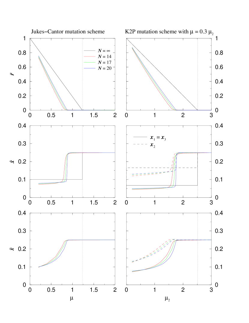
Figure 14: Comparison of population mean fitness $\bar{r}$, ancestral mean mutational distance $\hat{\bi{x}}$ and population mean mutational distance $\bar{\bi{x}}$ for different sequence lengths and the infinite system with truncation selection (23) with $x_{c}=0.1$. Left: JC mutation scheme, right: K2P mutation scheme with $\mu=0.3\mu_{2}$. The locations of the error thresholds in the infinite system are marked as vertical dotted lines.

Figure 14 compares the results for truncation selection obtained via the maximum principle (20) ($N=\infty$) with those obtained by calculating the largest eigenvalue and corresponding eigenvector of the symmetrized time-evolution operator $\widetilde{\bi{H}}$ for finite sequence length analogously to the data shown in Figure 8 for the quadratic symmetric fitness (22). On the left, one sees the data for the JC mutation scheme, whereas on the right, the results for the K2P model with $\mu=0.3\mu_{2}$ are shown. Here, it is obvious that even for rather small sequence length, the error thresholds are very sharp. However, keeping in mind the discontinuity of the truncation selection, this is not too surprising. One can see that the location of the error threshold does depend on the sequence length: The smaller the sequence length $N$, the more the error threshold is shifted to lower mutation rates. So although the sequence lengths considered here are large enough to warrant a sharp error threshold, they are too small to predict the location of the error threshold in the infinite system.

6.4.3 Distributions.

In the same way as for the quadratic symmetric fitness function (22), the ancestral and population distributions have been calculated for the truncation selection (23) and are shown in Figures 15 and 16. In contrast to Figures 9 to 11, which are the equivalent diagrams for the quadratic symmetric fitness function, every point in the sequence space is displayed as a separate cube, whose size is proportional to the fraction of individuals having that type in the ancestral and population distributions, respectively.

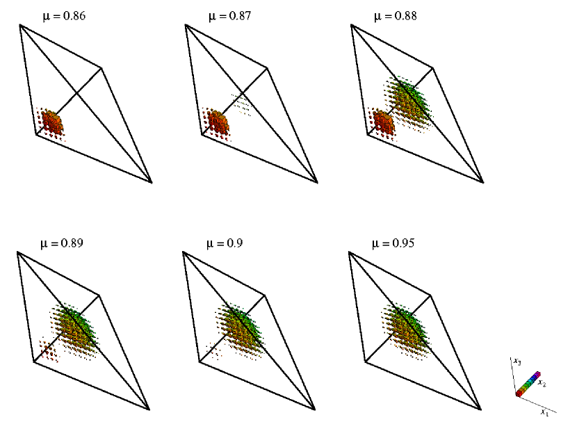
Figure 15: Ancestral distribution $\bi{a}$ for the JC mutation model with truncation selection (23) and $x_{c}=0.1$ with a sequence length of $N=20$ for mutation rates $\mu$ close to the error threshold.

Figure 15 shows the ancestral distribution of a system with sequence length $N=20$ and the JC mutation scheme for mutation rates close to the error threshold. For mutation rates below the threshold ($\mu\leq 0.86$), the ancestral distribution is an equidistribution in the “fit” part of the sequence space, where $\sum_{k}x_{k}\leq x_{c}$ and thus $r=1$. For mutation rates above the threshold ($\mu\geq 0.95$), the ancestral distribution is the equidistribution in the whole sequence space. The transition at the threshold is however interesting. Here, the distribution does not move smoothly from one equidistribution to the other, but in the intermediate states, the ancestral distribution is a superposition of the two equidistributions with an increasing proportion of the equidistribution on the whole sequence space.

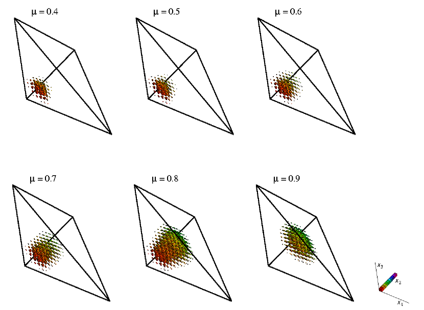
Figure 16: Population distribution $\bi{p}$ for the JC mutation model with truncation selection (23) and $x_{c}=0.1$ with a sequence length of $N=20$ for varying mutation rates $\mu$.

Figure 16 shows the population distribution for a system with the same parameters as shown in Figure 15, i. e., JC mutation model and truncation selection (23) with $x_{c}=0.1$ and sequence length $N=20$. Here, the transition from a localized distribution for small mutation rates to the equidistribution in sequence space looks far smoother (even apart from the far broader range of mutation rates over which it happens). The distribution as a whole shifts its centre until it reaches the equidistribution.

As the situation is very similar for general K2P mutation model (apart from a difference in mutation rates, cf. Figure 13, left), no distributions for a case with different mutation rates are shown.

7 Conclusion

In this paper we presented the model for sequence evolution introduced in [12], which takes into account the four-letter structure of DNA sequences. In [10], a maximum principle to determine the population mean fitness has been derived for this model, which is equivalent to the principle of minimum free energy in physical systems. Here, we used this maximum principle to investigate the phenomenon of error thresholds that are driven by mutation rate for a number of models.

The general mutation model in our setup is the Kimura 3ST mutation scheme, where it is accounted for one mutation rate for transitions and two mutation rates for the different types of transversions. In the analysis of the phase diagrams we focused on 2 simplifications of this model: Firstly, the Kimura 2 parameter model, where the two mutation rates for transversions are taken to be identical, and secondly, the Jukes-Cantor mutation model as a special case of the Kimura 2 parameter model where all three mutation rates coincide.

Inherent in our setup, there is a restriction to permutation-invariant fitness functions, where the fitness depends only on the number of mutations, i. e., the mutational distance $\bi{d}$, not on their position in the sequence. In principle, it is possible to consider any fitness function from this permutation-invariant class within our framework. Not all possible fitness functions give rise to error thresholds, for instance, with non-epistatic fitness functions, i. e., functions that are linear in the mutational distance $\bi{d}$, there exist no error thresholds. Here, we have focused on two simple examples of fitness functions that do cause error thresholds, namely (i) a fairly general quadratic symmetric (with respect to the components of the mutational distance $d_{i}$) fitness function and (ii) a truncation selection.

For these fitness functions, error thresholds can be found for certain parameter values. It has been argued (e. g. [5]), that the error threshold phenomenon, which was first described for a model with single-peaked landscape, might be an artefact of this highly unrealistic fitness function. Our results show, however, that they are not limited to this fitness, but occur for different types of fitness functions both smooth (the quadratic fitness) and discontinuous (truncation selection) ones. A certain degree of complexity is however needed for error thresholds, as there are none for a linear fitness. Therefore one can expect that more realistic fitness landscapes, which are more rugged and not of the permutation-invariant type, might show a rich error threshold behaviour. Hence error thresholds are a phenomenon that plays a role in evolution, as supported by recent experimental data [7, 6].

Apart from the ordered and disordered phases, which also occur in two-state models, a partially ordered phase has been observed [12], which differentiates only between purines and pyrimidines. This phase is directly dependent on the four-state nature of our model. However, as our analysis has shown, it is as well dependent on a certain symmetry of the fitness function, which comes naturally in the equivalent physical systems, but seems rather artificial in the biological setting, indicating that this phase, interesting though it may be, is of little significance in biology.

References

References

- [1] E. Baake, M. Baake, A. Bovier, and M. Klein. An asymptotic maximum principle for essentially linear evolution models. 2004. Preprint q-bio.PE/0311020.
- [2] E. Baake, M. Baake, and H. Wagner. Ising quantum chain is equivalent to a model of biological evolution. Physical Review Letters, 78(3):559–562, 1997. Erratum, Physical Review Letters 79 (1997), 1782.
- [3] E. Baake and W. Gabriel. Biological evolution through mutation, selection, and drift: An introductory review. In D. Stauffer, editor, Annual Reviews of Computational Physics VII, pages 203–264. World Scientific, Singapore, 2000.
- [4] R. Bürger. The Mathematical Theory of Selection, Recombination, and Mutation. Wiley, Chichester, 2000.
- [5] B. Charlesworth. Mutation-selection balance and the evolutionary advantage of sex and recombination. Genetical Research Cambridge, 55(3):199–221, 1990.
- [6] S. Crotty, C. E. Cameron, and R. Andino. RNA virus error catastrophe: Direct molecular test by using ribavirin. Proceedings of the National Academy of Sciences, 98(12):6895–6900, 2001.
- [7] E. Domingo and J. J. Holland. RNA virus mutations and fitness for survival. Annual Review of Microbiology, 51:151–178, 1997.
- [8] J. W. Drake, B. Charlesworth, D. Charlesworth, and J. F. Crow. Rates of spontaneous mutation. Genetics, 148(4):1667–1686, 1998.
- [9] M. Eigen. Selforganization of matter and the evolution of biological macromolecules. Naturwissenschaften, 58(10):465–523, 1971.
- [10] T. Garske and U. Grimm. A maximum principle for the mutation–selection equilibrium of nucleotide sequences. Bulletin of Mathematical Biology, 66(3):397–421, 2004. (Preprint physics/0303053).
- [11] J. Hermisson, O. Redner, H. Wagner, and E. Baake. Mutation selection balance: Ancestry, load, and maximum principle. Theoretical Population Biology, 62:9–46, 2002.
- [12] J. Hermisson, H. Wagner, and M. Baake. Four-state quantum chain as a model of sequence evolution. Journal of Statistical Physics, 102(1/2):315–343, 2001.
- [13] T. H. Jukes and C. R. Cantor. Evolution of protein molecules. In H. N. Munro, editor, Mammalian Protein Metabolism, pages 21–132. Academic Press, New York, 1969.
- [14] S. Karlin. A First Course in Stochastic Processes. Academic Press, New York, 1966.
- [15] J. G. Kemeny and J. L. Snell. Finite Markov Chains. Van Nostrand Reinhold Company, New York, 1960.
- [16] M. Kimura. A simple method for estimating evolutionary rate of base substitutions through comparative studies of nucleotide sequences. Journal of Molecular Evolution, 16:111–120, 1980.
- [17] M. Kimura. Estimation of evolutionary distances between homologous nucleotide sequences. Proceedings of the National Academy of Sciences USA, 78(1):454–458, 1981.
- [18] A. S. Kondrashov. Deleterious mutations and the evolution of sexual reproduction. Nature, 336:435–440, 1988.
- [19] I. Leuthäusser. An exact correspondence between Eigen’s evolution model and a two-dimensional Ising system. Journal of Chemical Physics, 84(3):1884–1885, 1986.
- [20] I. Leuthäusser. Statistical mechanics of Eigen’s evolution model. Journal of Statistical Physics, 48(1/2):343–360, 1987.
- [21] J. Maynard Smith and E. Szathmáry. The Major Transitions in Evolution. Freeman, Oxford, 1995.
- [22] T. Ohta and M. Kimura. A model of mutation appropriate to estimate the number of electrophoretically detectable alleles in a finite population. Genetical Research, 22:201–204, 1973.
- [23] D. L. Swofford, G. J. Olsen, P. J. Waddell, and D. M. Hillis. Phylogenetic inference. In David M. Hillis, Craig Moritz, and Barbara K. Mable, editors, Molecular Systematics, pages 407–514. Sinauer, Sunderland, 1996.
- [24] P. Tarazona. Error thresholds for molecular quasispecies as phase transitions: From simple landscapes to spin-glass models. Physical Review A, 45(8):6038–6050, 1992.
- [25] J. H. van Lint. Introduction to Coding Theory. Springer, Berlin, 1982.