Michaelis-Menten Dynamics in Complex Heterogeneous Networks

Abstract

Biological networks have been recently found to exhibit many topological properties of the so-called complex networks. It has been reported that they are, in general, both highly skewed and directed. In this paper, we report on the dynamics of a Michaelis-Menten like model when the topological features of the underlying network resemble those of real biological networks. Specifically, instead of using a random graph topology, we deal with a complex heterogeneous network characterized by a power-law degree distribution coupled to a continuous dynamics for each network’s component. The dynamics of the model is very rich and stationary, periodic and chaotic states are observed upon variation of the model’s parameters. We characterize these states numerically and report on several quantities such as the system’s phase diagram and size distributions of clusters of stationary, periodic and chaotic nodes. The results are discussed in view of recent debate about the ubiquity of complex networks in nature and on the basis of several biological processes that can be well described by the dynamics studied.

, and

1 Introduction

The discovery that many seemingly diverse systems, both natural and man-made, can be represented as networks with similar topological properties has driven a great body of research work in the last few years [1, 2, 3]. Network modeling has become a useful and common tool in fields as diverse as communication [4, 5, 6], biological [7, 8] and social systems [9]. For instance, biological applications of network modeling range from the design of new drugs [10] to a better understanding of basic cellular processes [7]. In technological networks such as the Internet and the world-wide-web, the challenges include the design of new communication strategies in order to provide faster access time to millions of users [11], the implementation of better algorithms for database exchange and information dissemination [12, 13], and the understanding of the topological features with the final goal of protecting the networks against random failures, intentional attacks and virus spreading [6, 14, 15, 16, 17, 18].

These networks are described by several characteristics. Among all the properties that can be studied, one usually finds that real-world networks are small-worlds (SW), which means that the average distance between two arbitrarily chosen nodes scales with the system size only logarithmically [2, 3]. Besides, the structural complexity of these networks is characterized by the number of interacting partners (connectivity $k$) of a given element (node). Surprisingly, the majority of real-world networks studied so far display a distribution of links that follows a power-law $P(k)\sim k^{-\gamma}$ (termed scale-free networks), with $\gamma\leq 3$ [1, 2].

Biological networks at all levels of organization are nowadays the subject of intense experimental and theoretical research. Recent analysis of protein-protein interaction networks has provided new useful insights into biological essentiality at this level of organization [19]. It is also believed that a better comprehension of gene and protein networks will help to elucidate the functions of a large fraction of proteins whose functions are unknown [20]. Moreover, it is a major challenge the discovery of how biological entities interact to perform specific biological processes and tasks, as well as how their functioning is so robust under variations of internal and external parameters [21, 22, 23].

It has been recently shown [24] that regulatory genes interact forming a complex interconnected network. This network is both directed and highly skewed for the yeast Saccharomyces cerevisiae. This means that there are a few regulatory genes that interact with many others but most of the genes only participate in a few processes. Another example in biology is given by metabolic networks. These networks are also directed and skewed. In this case, a large number of substrates (the nodes of the graph) are involved in a few metabolic reactions (the links) while a tiny fraction of substrates participate in a high number of reactions [25].

On the other hand, in the absence of conclusive experimental results, it is difficult to know what the interaction rules of, for instance, genetic networks actually are, although several experiments have proved that regulatory gene networks are highly nonlinear dynamical systems [26, 27]. This makes it clear that one should deal with both dynamical and structural complexity. Recently [28], we have studied the chaotic dynamics of a continuous gene-expression like model coupled to a complex heterogeneous network. In this paper, we fully characterize the different dynamical regimes observed. Specifically, we study numerically the steady, periodic and chaotic states that appear upon variation of the system’s parameters. The results obtained allow us to draw interesting conclusions about the robustness (hereafter intended as the ability of the system to avoid the phase space of chaotic dynamics) and behavioral richness of complex biological networks.

The rest of the paper is organized as follows. In section 2, we describe the network’s construction, introduce the model and explain the numerical procedure. Next, the different dynamical regimes are shown and analyzed in section 3. Finally, the last section rounds off the paper by discussing our results and giving the conclusions of the present study.

2 The Model

The model we will discuss in what follows is built in two layers. The first one refers to the topology of the underlying network while the second ingredient has to do with the dynamics of the network’s components. As noted before, the topology of two relevant biological networks has been recently shown to be very heterogeneous. This characteristic is shared by other networks in biology [3]. In addition, they are directed. Henceforth, we assume that each vertex of the underlying network corresponds to a biological entity and that the links stand for their interactions.

We construct the underlying network in the following way. Let $C_{ij}$ be the connectivity matrix of an undirected network built up following the Barabási and Albert model [30]. This recipe allows the generation of random scale-free networks with a degree distribution $P(k)\sim k^{-3}$ and an average connectivity $\langle k\rangle=2m$, being $m$ the number of new links added at each time step during the generation of the network (henceforth $m=3$ and $\langle k\rangle=6$). The elements of the matrix $C_{ij}$ are equal to $1$ if nodes $i$ and $j$ are connected and zero otherwise. Then, we transform $C_{ij}$ into the new matrix $W_{ij}$ describing directional interactions [29]. To this end, we look over the nonzero elements of $C_{ij}$ and with probability $p$ consider that the interaction $i\leftarrow j$ is inhibitory, $W_{ij}=-1$, and with probability $(1-p)$ it is excitatory, $W_{ij}=1$. Note that now the resulting matrix $W_{ij}$ is not, in general, symmetric anymore. In this way, the parameter $p$ controls the average output (input) connectivity of each node.

The second layer of the model has to do with the individual dynamics of each node in the underlying network. There is no model that incorporates all known facts about a given biological process and represents efficiently and accurately its complexity. Therefore, the development of a simplifying model is often essential in trying to understand the phenomenon under consideration. Here, we study a generic class of dynamical system that often appears in the biological context and discuss the results for two plausible biochemical processes, gene expression and reaction kinetics.

Consider that the activity of the nodes is described by the vector ${\bf G}(t)=\{g_{1}(t),g_{2}(t),\ldots,g_{N}(t)\}$, where $g_{i}$ ($i=1,\ldots,N$) accounts for the activity level of each individual node $i$ in a network made up of $N$ elements. The time evolution of ${\bf G}(t)$ is described by the following set of first-order differential equations [3, 32],

$$\frac{d{\bf G}(t)}{dt}=-{\bf G}(t)+{\bf F}({\bf G}(t)),$$ (1)

where ${\bf F}({\bf G}(t))$ is some nonlinear term where the interactions between the network’s elements are taken into account. Equation (1) includes continuous versions of Random Boolean Networks [33, 34] as well as continuous-time Artificial Neural Networks [35], both widely used to model periodic and chaotic dynamics in some biologically relevant situations. Additionally, we implement a continuous Michaelis-Menten description [3, 32, 36],

$$F_{i}({\bf G}(t))=\delta\frac{\Phi[h\sum_{j=1}^{k_{i}}W_{ij}g_{j}(t)]}{1+\Phi[h\sum_{j=1}^{k_{i}}W_{ij}g_{j}(t)]},$$ (2)

where $W_{ij}$ is the interaction matrix introduced before. Additionally, $\delta>0$ and $h>0$ are constants, $k_{i}$ is the connectivity of node $i$, and the function $\Phi(z)$ is defined as follows

$$\Phi(z)=\left\{\begin{array}[]{ll}0&\;\;\;\;\mbox{if $z\leq 0$}\\ z&\;\;\;\;\mbox{if $z>0$}\end{array}\right.$$ (3)

We have set $\delta=3$ hereafter and varied $h$. One can easily realize that the solutions ${\bf G}(t)$ for non-negative initial conditions remain bounded for all $t>0$: As $F_{i}({\bf G}(t))$ is bounded above by $\delta$, $dg_{i}(t)/dt<0$ whenever $g_{i}(t)>\delta$. Also, if $g_{i}(t)=0$ then $dg_{i}(t)/dt=F_{i}({\bf G}(t))\geq 0$, so that the activities cannot become negative.

The dynamics of the system defined as before is determined by only two parameters, $h$ and $p$. One controls the degree of nonlinearity and the other the topological properties of the network, respectively. We have performed extensive numerical simulations of the set of equations (1-2). Starting from small values of $h$, the time evolution of the local dynamics $g_{i}$ is obtained by means of a 4$th$-order Runge-Kutta integration scheme [37]. The set of simulations carried out screens the parameter space $(h,p)$, where $h$ goes from $1$ to $10$ and $p$ from $0$ to $1$. For each pair $(h,p)$, different realizations corresponding to many initial conditions and network realizations were performed.

This dynamics turns out to be very rich and, depending on the values of $p$ and $h$, three different asymptotic dynamical regimes are observed, characterized by stationary, periodic and chaotic attractors. All three states may even coexist in a given network realization, each in different islands or clusters. Islands are subnetworks that are interconnected through nodes which have evolved to null activity, and so (asymptotically) their dynamics are effectively disconnected.

While stationary and periodic states point to regions of the parameter space where real biological networks might operate, the existence of chaotic dynamics would be, in general, inconsistent with the reproducibility of experimental observations in living organisms. Hence, we have characterized all possible responses of the system under variations of both $h$ and $p$ and monitored the evolution of $g_{i}(t)$, the probabilities of ending up in either chaotic or periodic dynamics as well as the distribution of clusters or islands of nodes displaying such behaviors. Moreover, due to recent interest in what is known as network motifs, we have also analyzed the topological features of the clusters exhibiting non-stationary behavior.

The computations presented in the rest of the paper were developed following this sequence:

• The initial values of $g_{i}$ are taken from a uniform distribution in the interval $(0,1)$.

• First integration of the equations is performed using a $4^{th}$ order Runge-Kutta scheme [37]. The total integration time is large compared with the transient.

• Check the dynamical state of the network. If all the nodes are in a steady state we try another initial configuration; if there are dynamical nodes go to the next stage.

• Check the connectivity between the dynamical nodes in order to obtain the dynamical subnetworks (islands).

• Second integration for calculating the largest Lyapunov exponent $\lambda$ [40]. If $\lambda>5\cdot 10^{-3}$ the dynamics is considered chaotic. If $\lambda<5\cdot 10^{-3}$ we look at the frequency of the periodic motion.

• Repeat stages (i)-(v) for different initial conditions and realizations of the network.

We have generated networks of sizes ranging from $N=100$ to $N=300$ nodes. At each value of $p$ and $h$, we have performed at least $1000$ iterations of the above procedure. The time step in the integration scheme was fixed to $10^{-4}$. We incorporate later on a further criterion in order to obtain the values of the frequencies of the periodic states.

3 Dynamical regimes

Figure 1: Probabilities of having chaotic, $P_{ch}$ or periodic $P_{per}$ behavior as a function of the topological parameter $p$. The value of $h$ has been set to $4$ and the system is made up of $N=300$ nodes. See the text for further details on the definitions.

The individual dynamics of the nodes is not uniform across the entire network due to the heterogeneity in the initial conditions and that of the underlying networks. While some nodes reach a stationary state, others follow periodic orbits and even chaotic behavior. The following argument explains how this can easily happen. If a node $i$ is such that $W_{ij}=-1$ for all $j$, then its activity will tend to zero. The same will happen for those nodes $l$ such that the positive $W_{lj}$ occur for $j$’s of the previous kind, etc… Now, two subnetworks connected between them through nodes whose activity dies out will become effectively disconnected, and so their dynamics are asymptotically independent. The network is then dynamically fragmented into islands.

A simple way in which the overall dynamics of the network can be described is through the computation of the largest Lyapunov exponent $\lambda$. Once we have obtained $\lambda$, we define the probability that a given dynamical regime is observed. As they are complementary, we define only two probabilities. Namely, the probability that the network displays chaotic behavior, $P_{ch}$, is the fraction of the total number of realizations in which at least one node ends up in a chaotic state yielding a positive value of $\lambda$. On the other hand, if $\lambda\leq 0$, the system does not end up in a chaotic regime and only stationary and/or periodic islands are observed. Consequently, the probability that no chaotic behavior is attained, but periodic orbits are observed, $P_{per}$, is given by the portion of the total number of realizations in which $\lambda\leq 0$ and there is at least one periodic orbit.

Figure 1 shows the two probabilities as a function of the topological parameter $p$ for a fixed value of $h=4$ and $N=300$. Two different threshold values for $p$ can be observed, mainly determined by $P_{per}$, $p_{1}\approx 0.2$ and $p_{2}\approx 0.95$. The first region $p<p_{1}$ corresponds to the case in which most of the interactions are excitatory and the individual dynamics are described by frozen steady states (either $g_{i}=0$ or $g_{i}\geq 0$). On the other hand, when the interactions become predominantly inhibitory ($p>p_{2}$), the activity of the nodes dies out due to the damping term in Eq. (1). In the intermediate region, $p_{1}<p<p_{2}$, all types of behaviors (stationary, periodic and chaotic) are achieved.

3.1 Stationary states

The simplest case of stationary state is the solution in which all the nodes remain inactive, i.e. $g_{i}=0$ for all $i$. Note that this is always a solution of the equations of motion, irrespective of the parameter values. As a matter of fact, for $h=0$, or $h\neq 0$ but $p=1$, the state of inactivity (or rest state) is the unique asymptotic solution for any non-negative initial conditions. However, for $h\neq 0$ and $p\neq 1$ other asymptotic solutions with islands of positive activity generically coexist.

Figure 2: Probability $P_{trans}$ that the uniform state of node inactivity becomes unstable for some value of $h$, as a function of the parameter $p$. $10^{4}$ different realizations have been used for each value of $p$.

Depending on the specific network realization (i.e. the matrix $W_{ij}$), the rest state can become unstable when the value of $h$ is increased from zero. This will occur for the value $h=\tilde{h}$ at which the largest eigenvalue (among those associated to eigenvectors such that all their components have the same sign [38]) of the matrix $-\delta_{ij}+\delta hW_{ij}$ becomes positive. Then $\tilde{h}$ is determined as $1/(\delta\lambda_{max})$, where $\lambda_{max}$ is the largest eigenvalue of $W_{ij}$, provided $\lambda_{max}>0$ (no instability of the rest state will occur if $\lambda_{max}\leq 0$). In Fig. 2 we show the probability $P_{trans}$ that the rest state becomes unstable for some value of $h$, as a function of the parameter $p$. This probability has been estimated from the computation of $\lambda_{max}$ for $10^{4}$ different realizations of $W_{ij}$ for each value of $p$. Though for most values of $p$ the rest state remains stable at all values of $h$, in $75\%$ (or more) of the realizations, it coexists in phase space with other attractors, so that only a basin of initial conditions evolves to this state.

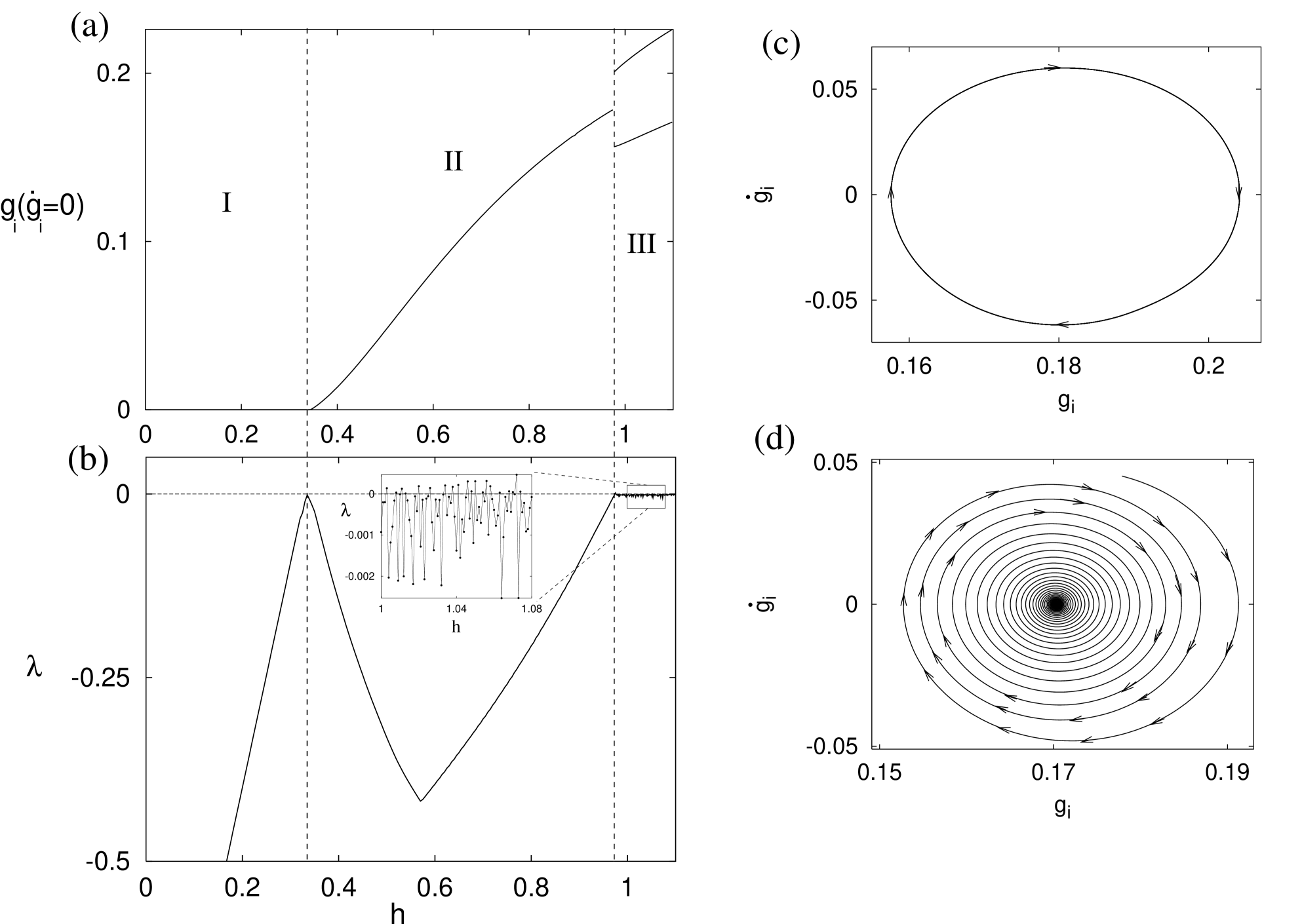
Figure 3: (a) Dependence of the quantity $g_{i}[\dot{g}_{i}=0]$ (activity level when its first derivative is zero) of a single node with the parameter $h$. This node belongs to a cluster which undergoes two bifurcations when increasing the value of $h$ starting from the rest state configuration of the whole network at $h=0$. In the first bifurcation ($h\simeq 0.345$) a cluster of nodes in a stationary state with non-zero activity level merges. When $h\simeq 0.976$ the nodes of this cluster end in a periodic attractor. The evolution of the largest Lyapunov exponent of the network as $h$ is increased is plotted in (b) showing the two bifurcations. (c) Periodic trajectory in the portion of the phase space corresponding to the node of figure (a), the value of $h$ is $0.98$. (d) Decay of the activity level of the same node to the stable fixed point for $h=0.97$ (just before the second bifurcation) when the initial condition of the network is the periodic solution shown in (c).

The rest state destabilizes typically through a transcritical bifurcation [39], where an unstable branch of stationary solutions exchanges stability with the rest branch (see Fig. 3a). The computed largest Lyapunov exponent shows a variation with $h$ as in Fig. 3b near $h\simeq 0.345$: it approaches zero (from negative values) at the bifurcation parameter value, and then decreases indicating that now the attractor belongs to the new stable stationary branch, in which the nodes of a cluster display non-zero activity. As shown in Fig. 3a, the activity of these nodes typically increases with $h$. Eventually, this state becomes unstable for larger values of $h$, typically through a Hopf bifurcation (either inverse or direct) to a periodic state in which the activities oscillate (Fig. 3c) regularly in time.

3.2 Periodic states

The observation that both $P_{per}$ and $P_{ch}$ in figure 1 are zero outside the interval $[p_{1},\;p_{2}]$ of values of the parameter $p$ clearly indicates that non-stationary activity is the result of the interplay between excitatory and inhibitory interactions in the network.

Figure 4: Time series for four different nodes exhibiting periodic dynamics. Time is in dimensionless units and starts just after the transient period. The value of $p$ is $0.7$ and $N=100$.

Figure 5: Probability that a node with periodic dynamics converges to an orbit of angular frequency $\omega_{per}$ (in arbitrary units). The results are averaged over different network realizations and at least 100 different initial conditions for a network of $N=100$ nodes and $p=0.7$. $h$ has been fixed to $4$.

In Fig. 4, we have plotted the time profiles of four different nodes in a periodic regime within the same island. One observes out of phase oscillations which reflect the existence of inhibitory interactions: the growth of the activity in the node $j$ inhibiting node $i$ ($W_{ij}=-1$) leads eventually to a null value of $F_{i}({\bf G}(t))$, thus to an exponential (free) decay of the activity of node $i$, until it is triggered again (due to the decay of the activity of inhibitory interactions and/or the increase of the excitatory nodes’ activity). As the free decay of activity has an associated time scale of order unity, one should expect values of this order for the period of oscillations.

This expectation is confirmed by computing the frequency distribution of nodes whose dynamics converge to a periodic cycle for different realizations. The numerical procedure is as follows: First, we identify the realizations in which the largest Lyapunov exponent is zero. Then, we focus on the nodes for which $dg/dt\neq 0$. Once identified, a vector ${\bf T}_{n}^{i}=\{t_{1}^{i},t_{2}^{i},\ldots,t_{n}^{i}\}$ is constructed and stored for every periodic dynamics $g_{i}$. The $t_{j}^{i}$’s stand for the times fulfilling the conditions $g_{i}(t_{1}^{i})=g_{i}(t_{2}^{i})=\ldots=g_{i}(t_{n}^{i})$ and $dg_{i}(t_{1}^{i})/dt=dg_{i}(t_{2}^{i})/dt)=\ldots=dg_{i}(t_{n}^{i})/dt$ [41]. In this way, after verifying that $t_{j}^{i}-t_{j-1}^{i}$ is constant, the period of the corresponding $i$-orbit is given by this constant.

In Fig. 5, we show the probability that a periodic cycle has an angular frequency $\omega_{per}$. As shown in the figure, it is very likely that the frequency of the activity of a periodic island lies around $\omega_{per}=1$. It is also of interest that $P(\omega_{per})$ is not symmetric, but biased towards larger frequency values. It is difficult to figure out an explanation to this behavior. It may probably have to do with the spatial distribution of the nodes and the specific value of $p$ which controls the average number of input and output connections a node has.

3.3 Chaotic states

Figure 6: Time series for five different nodes exhibiting chaotic dynamics. Time is in dimensionless units and starts just after the transient period. The value of $p$ is $0.7$ and $N=100$.

Although in general not desirable from a biological point of view, systems displaying chaotic behavior are always of interest [40]. Moreover, the existence of chaotic dynamics does not only depend on parameters associated to the dynamics employed (as in most of the studies performed so far regarding chaotic dynamics), but more important, it is the result of a complex interplay between the dynamical and structural (topological) complexity. We next summarize the results obtained for the chaotic dynamics of the system.

The two threshold values in the phase diagram for the chaotic regime depicted in Fig. 1 depends on $h$. Clearly, as the degree of nonlinearity increases, chaotic behavior appears more frequently, which translates in a larger maximum for $P_{ch}$. On the other hand, although we have used a small system size, the values of $p_{1}$ and $p_{2}$ seem to be robust when $N$ grows. This means that the results obtained are meaningful for larger systems since the onset and the end of the chaotic phase are $N$ independent. In Fig. 6 we have represented the time profile of five different nodes in the chaotic regime. Time units refer to integration steps and the origin of the time scale begins just after the transient period. The system’s parameters are as indicated. Note that although all these nodes are in the same chaotic island, the patterns of activity are quite different and the amplitudes of the chaotic signal (and the shape of the curves) are distinguishable.

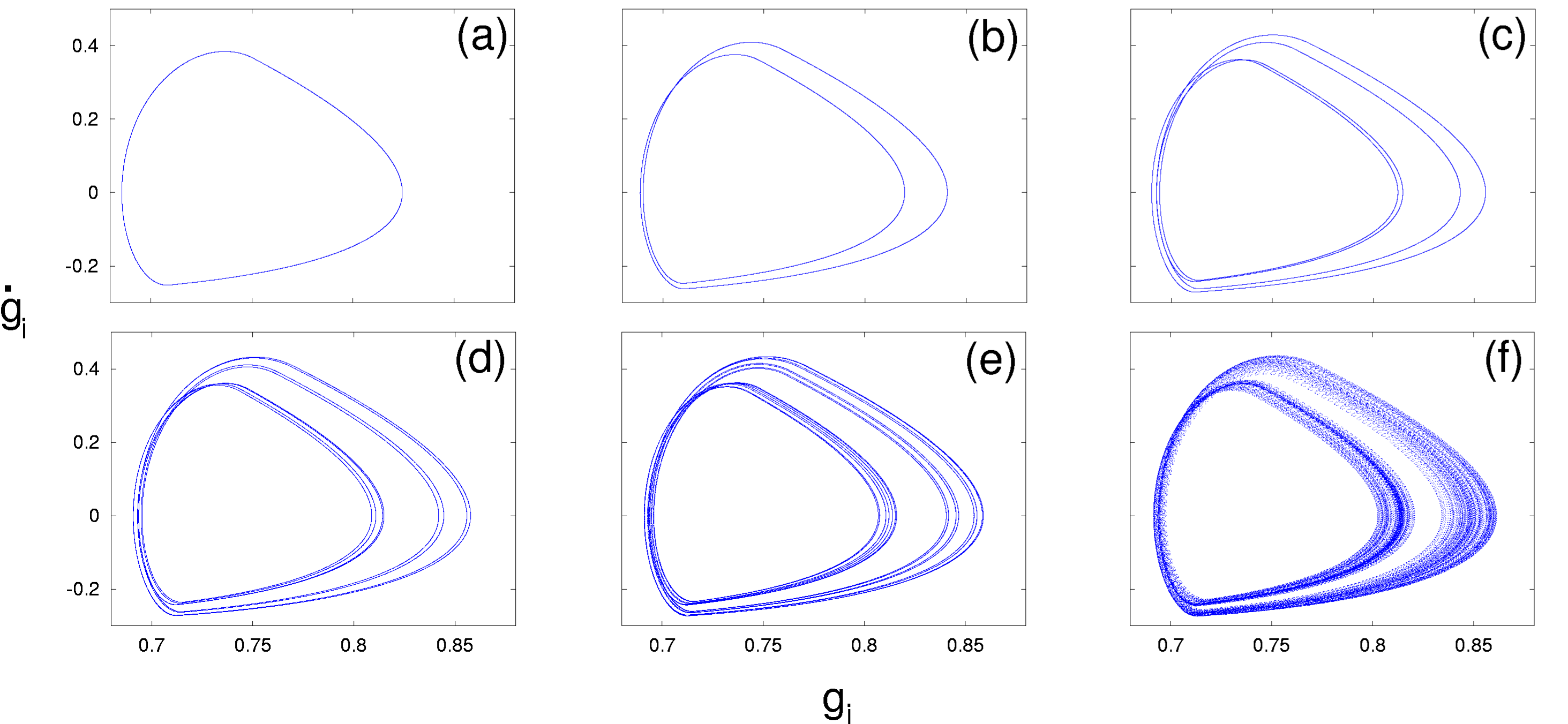
Figure 7: Phase space of a node ending up in a chaotic state as the value of $h$ is increased. Successive period doublings starting from a periodic cycle can be appreciated. The values of $h$ (from (a) to (f)) are: $5.30$, $5.50$, $5.63$, $5.65$, $5.66$, $5.68$, respectively. Other network parameters are as in Fig. 6.

It is also of interest to know how the chaotic regime is attained. The origin of different dynamical patterns is related to the values of $p$ and $h$. First, we study the transition to chaos from periodic states. We have traced the route to chaos [28] by picking up a node at random among the chaotic ones. By increasing the value of $h$ at intervals of $\Delta h=0.02$, we recorded the local maxima of $g_{i}$ in the corresponding time series. The results reveal that the chaotic regime is reached through the period-doubling cascades mechanism [28].

As an evidence of the period-doubling mechanism, Fig. 7 shows the phase space diagrams of the node’s activity as $h$ is increased. For small values of $h$, the node is in a periodic cycle, which doubles its period successively until it reaches the chaotic phase. This corroborates that when $h$ and $p$ allows for a large value of $P_{ch}$, the behavior of the system is dominated by dynamical states (either periodic or chaotic). Moreover, the fact that $\sum P_{ch}+P_{per}$ is large indicates that nodes which are not in a chaotic state may be in the route to it. In other words, in this regime of parameters, when a given realization has no chaotic islands, it is very likely that it has periodic clusters.

Up to now, we have described the activity patterns in terms of their dynamical properties. However, one of the most interesting aspects of many biological networks is that their topology is highly heterogeneous. There are a few nodes which interact with many others. This should have some bearings in the results obtained. In the next section, we round off our numerical analysis of the model by correlating the dynamical properties unraveled with the network’s topological features.

3.4 Structural properties of dynamical regimes

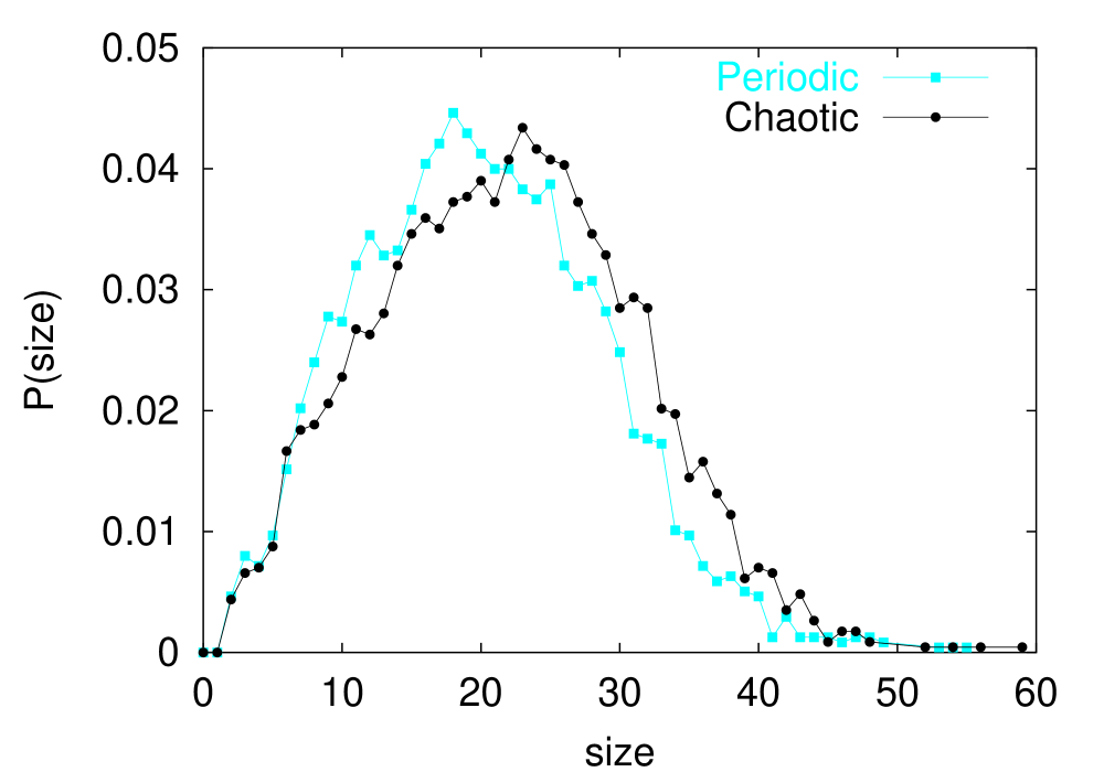
Figure 8: Probability that a connected cluster of nodes displaying either chaotic or periodic behavior has a given size (in number of nodes forming the cluster). Although the curves correspond to two radically different behaviors, they are very similar. Network parameters are as in Fig. 5.

In order to characterize the structural properties of distinct dynamical regimes, we focus on some magnitudes. The first and simplest structural characterization is given by the distribution of nodes exhibiting either periodic or chaotic dynamics, i.e. the histograms of periodic (and chaotic) cluster sizes.

The results are shown in Fig. 8, where the size distribution of the two dynamical behaviors are drawn for $N=100$ elements, $p=0.7$, and $h=4$. Apart from slight fluctuations in the maxima of both curves, it is apparent the existence of a mean average cluster size for chaotic and periodic islands, though the dispersion around this mean value is relatively large. The fact that both curves almost collapse into a single one indicates that the clusters of periodic nodes are the same that later on, by increasing $h$ at fixed $p$, evolve to a chaotic state. Moreover, since the largest clusters are made up of roughly half of the network’s constituents, it is highly improbable that the entire system displays the same behavior. In other words, the fragmentation of the network into islands of independent dynamics appears as one of the most characteristic features of this model. In Fig. 9, we show four different clusters corresponding to nodes with chaotic dynamics. As one can see, no typical structure appears, even for clusters of comparable sizes, except that all of them have a relatively small value of the cluster average connectivity.

In addition, we would like to add a few sentences about network motifs, a subject that has become of utmost interest in biological and other networks due to its implications in modularity and community structures [19]. Motifs are small graph components or loops that appear more frequently than in a random network with identical degree distribution [3, 42]. We have found no correlation between the clusters of periodic or chaotic behavior with the structural properties of the underlying network. In particular, chaotic or periodic clusters do not follow a universal topological pattern, contrary to what one may expect from other studies on network evolution and motifs (see, for instance, Maslov et al. in ref. [3], and [43]). We believe that this is due to the fact that the underlying network, although heterogeneous and with directed interactions, is a random scale-free network, for which the probability that a motif exists is much lower than in real biological networks.

Figure 9: Examples of chaotic clusters (or islands) whose size distribution is reported in the previous figure. As one can see, no typical structure arises regardless of the existence of a well-defined average cluster size.

The heterogeneity of the underlying network allows us to further scrutinize the correlations between structural and dynamical properties. In particular, it is also of interest to elucidate what nodes take part in each regime according to their connectivities. We have anticipated in [28] that highly connected nodes are less likely in a chaotic regime. However, due to the small size of the networks, the results there shown are biased by the huge fluctuations in the tail of the connectivity distribution. It is then advisable to work instead with the cumulative distribution in order to rule out as much as possible the noise in the tail of $P(k)$. We have monitored the probability that a node with connectivity $k$ displays either chaotic or periodic behavior. These probabilities, $\Pi_{chaotic}$ and $\Pi_{periodic}$ respectively, are defined as the ratio between the number of nodes with degree $k^{\prime}$ greater than or equal to $k$ that end up in a chaotic (periodic) regime and the total number of nodes with connectivity $k^{\prime}\geq k$ averaged over many realizations. Figure 10 shows the results obtained.

Figure 10: Probability of having periodic or chaotic behavior in a node of connectivity $k$. The figure indicates that dynamical regimes are well differentiated by connectivity classes. Network parameters are as of Fig. 6.

Two interesting issues are worth mentioning. On one hand, the fact that the chaotic phase is reached through the doubling-period cascade mechanism leads us to expect that $\Pi_{chaotic}$ and $\Pi_{periodic}$ behave in a similar fashion, which is confirmed in the figure. In other words, nodes that are not chaotic are in cycles that eventually will double their periods (as $h$ is increased) until chaotic states are attained. This means that if each cycle is identified with a variety of intracellular tasks, the transition from one cycle to another and to a chaotic phase is continuous and does not occur suddenly. On the other hand, the results in Fig. 10 points to the differences in the nodes’ dynamics according to their connectivities. In particular, apart from an apparent maximum attained around the mean average connectivity, the results show that the more connected a node is the less likely it is in a chaotic regime or in the route to it (this is more clearly appreciated for $\Pi_{periodic}$).

4 Discussions and Conclusions

A large number of systems have been studied in the last several years from the network perspective [2, 3, 6]. This approach has allowed the understanding of the effects of complex topologies in many well-studied problems. By comparing the results obtained with other topologies and those for real graphs in processes such as the spreading of epidemic diseases [15, 16] or rumors [12] and the tolerance of complex networks to random failures and attacks [14], we have realized that topology plays a fundamental role.

As for biological systems, a very rich behavioral repertoire is well documented [36]. Cycles in biological systems range from circadian clocks to the oscillations observed in the concentration of certain chemicals, for instance, in biochemical reactions such as glycolysis. On the other hand, the molecular basis for chaotic behavior have also been discussed, though chaotic behavior is probably not a relevant issue in biology as intrinsic noise makes it difficult to isolated truly chaotic regimes with current experimental techniques. The dynamics studied in this work, however, could plausible describe at least to biological scenarios, namely, gene expression and reaction kinetics in metabolic networks.

The description of gene dynamics has to rely necessarily on models that are only an approximation to that of real genes. However, there are several successful approaches to the individual dynamics of gene expression. Since its introduction by Kauffman several decades ago, one of the most studied class of models are the Random Boolean Networks (RBNs) [31], which have been shown to lead to some predictable properties and guided our understanding towards more complex descriptions. Our model belongs to a generalized class of RBNs. It takes into account the fact that genome regulation involves continuous concentrations of RNA and proteins. The latter class has also been extensively studied in the last years (see, for instance, Solé and Pastor-Satorras in ref. [3] and references therein). In this context, each vertex would represent a regulatory gene and the links would describe their interactions. In other words, two nodes at the ends of a link are considered to be transcriptional units which include a regulatory gene. One of these end-nodes can be thought of as being the source of an interaction (the output of a transcriptional unit). The second node represents the target binding site and at the same time the input of a second transcriptional unit.

In genetic network models, it is known that at least for RBNs, the results are affected by the type of Boolean functions used, the number of network’s constituents and the average connectivity (mainly input connectivity) of the genes [31]. Recently, it has also been demonstrated that the degree distribution matters [44]. In our continuous model, results obtained for homogeneous random networks [28] indicate that the values of $p$ for the onset of chaos change as well. On the other hand, as pointed before, gene networks are constrained by their required functional robustness. Therefore, as chaos represents a long-term behavior that exhibits sensitive dependence on initial conditions, real biological gene networks must not systematically operate in the parameter region where the existence of chaotic attractors is likely. By studying simplified models as the one implemented here $-$ the intrinsic complexity of the problem does not allow for a complete and detailed description of real gene dynamics $-$, one can infer the region of the parameter space (i.e. $(p,h)$) that better describes gene networks. Based on this hypothesis, by exploring magnitudes as the one represented in Fig. 1, we would either guess dynamical interaction rules or provide hints for the experimental validation of the structural topology of real networks. The latter seems more feasible due to latest developments in microarray technologies, biocomputational tools, and data collection software.

On the theoretical side, the continuous model employed here shares some features with respect to those seen in RBNs. For instance, although $p_{1}$ depends on the specific value of $h$ entering Eq. (2), it lies in the interval $(0.2,0.6)$ for $1\leq h\leq 10$. The existence of a relevant average input connectivity $\langle\kappa\rangle$ between $2$ and $3$ for homogeneous networks in the context of RBNs was pointed out several years ago by Kauffman [31], who later suggested that this range could be even larger (up to $\langle\kappa\rangle=5$) if the Boolean functions are biased toward higher internal homogeneity [45]. Our results provide another possible scenario for such a high value of $\langle\kappa\rangle$. Namely, that heterogeneous distributions together with highly nonlinear interactions allow for larger $\langle\kappa\rangle$ values. Moreover, contrary to what has been observed in RBNs, $p_{1}(h)$ depends only slightly on the system size, which makes the previous analysis meaningful for larger networks.

As for metabolic networks, the system of differential equations, Eqs. (1-2), represents one of the most basic biochemical reactions, where substrates and enzymes are involved in a reaction that produces a given product. In this context, there are several important issues as how fast the equilibrium is reached, how the concentration of substrates and enzymes compare, etc. Besides, it is known that in a large number of situations, some of the enzymes involved show periodic increments in their activity during division, and these reflect periodic changes in the rate of enzyme synthesis. This is achieved by regulatory mechanisms that necessarily require some kind of feedback control as that emerging in our model. Obviously, there is a vast literature on this kind of process, but the point here is that the real topological features of the underlying metabolic network [25] has not been taken into account, and as far as dynamics is concerned, they should be incorporated in current models. We are planning to address this issue in the future.

In summary, we have studied a Michealis-Menten like dynamical model on top of complex heterogeneous networks with directed links. The free parameters of the model allowed us the full exploration of the phase diagram of the system’s dynamics under different dynamical and structural conditions. The results obtained point to a rich behavioral repertoire with stationary, periodic and chaotic regimes. A direct comparison with experiments is a tough task, especially, because experimental results are only now becoming available. However, we anticipate several features of interest such as that heterogeneous networks reduces the parameter range in which the existence of chaotic behavior is likely and that distinct behaviors correlate with connectivity classes. These suggestions could be tested when more experimental information becomes available. Our study may help understand biological processes such as gene expression and reaction kinetics with the tools of network modeling and nonlinear dynamics. Finally, we would like to point out that further numerical simulations with other random scale-free networks with lower exponents $\gamma$ (i.e., more heterogeneous nets) [46], suggest that the main conclusions drawn here do not significantly depend on $\gamma$.

5 Acknowledgments

We thank F. Falo, P. J. Martínez and J. L. García-Palacios for fruitful discussions and suggestions. Y. M. thanks S. Boccaletti for suggestions. J. G-G acknowledges financial support of the MECyD through a FPU grant. Y. M. is supported by a BIFI Research Grant and by MCyT through the Ramón y Cajal program. This work has been partially supported by the Spanish DGICYT projects BFM2002-01798 and BFM2002-00113.

References

- [1] S. H. Strogatz, Nature (London) 410, 268 (2001).
- [2] S. N. Dorogovtsev and J. F. F. Mendes, Evolution of Networks. From Biological Nets to the Internet and the WWW, Oxford University Press, Oxford, U.K., (2003).
- [3] See for instance, Handbook of Graphs and Networks: From the Genome to the Internet, eds. S. Bornholdt and H.G. Schuster (Wiley-VCH, Berlin, 2002).
- [4] M. Faloutsos, P. Faloutsos, and C. Faloutsos, Proceedings of the ACM, SIGCOMM [Comput. Commun. Rev. 29, 251 (1999)]
- [5] A. Vázquez, R. Pastor-Satorras, and A. Vespignani, Phys. Rev. E 65, 066130 (2002).
- [6] R. Pastor-Satorras and A. Vespignani, Evolution and Structure of the Internet, Cambridge University Press, Cambridge, U.K., (2004).
- [7] H. Jeong, S. P. Mason, A.-L. Barabási, and Z. N. Oltvai, Nature (London) 411, 41 (2001).
- [8] R. V. Solé, and J. M. Montoya, Proc. R. Soc. London B 268, 2039 (2001).
- [9] M. E. J. Newman, Proc. Natl. Acad. Sci. U.S.A. 98, 404 (2001).
- [10] R. Albert, H. Jeong, and A.-L. Barabási, Nature 409, 542 (2000).
- [11] P. Echenique, J. Gómez-Gardeñes, and Y. Moreno, Phys. Rev. E, 70, 056105 (2004).
- [12] Y.Moreno, M. Nekovee, and A. Vespignani, Phys. Rev. E, 69, 055101(R) (2004).
- [13] Y.Moreno, M. Nekovee, and A. F. Pacheco, Phys. Rev. E, 69, 066130 (2004).
- [14] D. S. Callaway, M. E. J. Newman, S. H. Strogatz, and D. J. Watts, Phys. Rev. Lett. 85, 5468 (2000).
- [15] R. Pastor-Satorras, and A. Vespignani, Phys. Rev. Lett. 86, 3200 (2001).
- [16] Y. Moreno, R. Pastor-Satorras, and A. Vespignani, Eur. Phys. J. B 26, 521 (2002).
- [17] Y.Moreno, J. B. Gómez, and A. F. Pacheco, Phys. Rev. E, 68, 035103(R) (2003).
- [18] A. Vázquez and Y.Moreno, Phys. Rev. E, 67, 015101(R) (2003).
- [19] H. Jeong, Z. N. Oltvai, and A.-L. Barabási, ComplexUs 1, 19 (2003).
- [20] A. Vázquez et al., Nat. Biotech. 21, 697 (2003).
- [21] M. A. Savageau, Nature 229, 542 (1971); Nature 258, 208 (1975).
- [22] U. Alon, M. Surette, N. Barkai, and S. Leiber, Nature 397, 168 (1999).
- [23] A. Eldar et al., Nature 419, 304 (2002).
- [24] J. M. Stuart et al., Science 302, 249 (2003).
- [25] H. Jeong and B. Tombor and R. Albert and Z. Oltvai and A.-L. Barabási, Nature (London) 407, 651 (2000).
- [26] J. L. DeRisi, V. R. Iyer, and P. O. Brown, Science 278, 680 (1997).
- [27] H. Tao, C. Bausch, C. Richmond, F. R. Blattner, and T. Conway, J. Bacteriol. 181, 6425 (1999).
- [28] J. G. Gardeñes, Y. Moreno, and L. M. Floría, e-print archive q-bio.MN/0404029 (2004).
- [29] Note that the directness of the network is here used in the sense that the interactions between any two given elements can be excitatory or inhibitory. However, by construction, it is implicitly assumed that if node interacts with node the opposite also holds, i.e., node also interacts with though this interaction could be in a different way. We acknowledge that this is a simplification of real networks and plan to extend our study to more realistic network topologies.
- [30] A.-L. Barabási, and R. Albert, Science 286, 509 (1999); A.-L. Barabási, R. Albert, and H. Jeong, Physica A 272, 173 (1999).
- [31] S. Kauffman, Origin of Order (Oxford University Press, Oxford, 1993).
- [32] R. V. Solé, I. Salazar-Ciudad, and J. Garcia-Fernández, Physica A 305, 640 (2002).
- [33] T. Mestl, R. J. Bagley, and L. Glass, Phys. Rev. Lett. 79, 653 (1997).
- [34] L. Glass and C. Hill, Europhys. Lett. 41, 599 (1998).
- [35] J. J. Hopfield, Proc. Natl. Acad. Sci. U.S.A. 81, 3088 (1984).
- [36] J. D. Murray, Mathematical Biology I: An Introduction (3rd Edition, Springer-Verlag, Berlin, 2002)
- [37] See for example, Numerical Recipes (Cambridge University Press, Cambridge, 1999).
- [38] Note that has a jump discontinuity in first partial derivatives at the rest state. Thus we consider the matrix of right-handed partial derivatives, and then only pay attention to tangent space vectors which do not bring the system into the region of negative activities.
- [39] R. Seydel, Practical Bifurcation and Stability Analysis (Springer, New York, 1994).
- [40] H. G. Schuster, Deterministic Chaos. An introduction (Wiley-VCH, 1995).
- [41] Since the integration is done at fixed time intervals, a further numerical check is impossed. Namely, and .
- [42] R. Milo, S. Shen-Orr, S. Itzkovitz, N. Kashtan, D. Chklovskii and U. Alon, Science 298, 824 (2002).
- [43] S. Wuchty, Z. N. Oltvai, and A. -L. Barabási, Nat. Genet. 35, 176 (2003).
- [44] C. Oosawa, and M. A. Savageau, Physica D 170, 143 (2002).
- [45] S. E. Harris, B. K. Sawhill, A. Wuensche, and S. Kauffman, Santa Fe Institute 97-05-039, 1997.
- [46] J. G. Gardeñes, Y. Moreno, and L. M. Floría, Biophysical Chemistry, in the press (2005).