Organization of ecosystems in the vicinity of a novel phase transition

Abstract

It is shown that an ecosystem in equilibrium is generally organized in a state which is poised in the vicinity of a novel phase transition.

An ecological community consists of individuals of different species occupying a confined territory and sharing its resourcesMacArthur and Wilson (1967); May (1975); Levin (2000); Wilson (2002). One may draw parallels between such a community and a physical system consisting of particles. In this letter, we show that an ecosystem can be mapped into an unconventional statistical ensemble and is quite generally tuned in the vicinity of a phase transition where biodiversity and the use of resources are optimized.

Consider an ecological community, represented by individuals of different species occupying a confined territory and sharing its common resources, whose sources (for example, solar energy and freshwater supplies) depend on the area of the territory, its geography, climate and environmental conditions. The amount of these resources and their availability to the community may change as a result of human activity and natural cataclysms such as climate change due to global warming, oil spills, deforestation due to logging or volcanic eruptions.

Generally, species differ from each other in the amount and type of resources that they need in order to survive and successfully breed. One may ascribe a positive characteristic energy intake per individual, $\varepsilon_{k}$, of the $k$-th species ($0<\varepsilon_{0}<\varepsilon_{1}<\dots$), which ought to depend on the typical size of the individualSchmidt-Nielsen (1984); Calder III (1984); McMahon and Bonner (1983); Peters (1983). The individuals of the $k$-th species play the role of particles in a physical system housed in the energy level $\varepsilon_{k}$.

We make the simplifying assumption that there is no direct interaction between the individuals in the ecosystem. Our analysis does not take into account predator-prey interactions but rather focuses on the competition between species for the same kind of resources.

In ecology, unlike in physical systems where one has a fixed (average) number of particles and an associated average energy of the system, one needs to define a new statistical ensemble. One may define the maximum amount of resources available to the ecological community to be $E_{max}$. The actual energy used by the ecosystem, $\langle E\rangle$, can be no more than $E_{max}$

$$E_{max}=T+\langle E\rangle$$ (1)

and, strikingly, as shown later, the energy imbalance, $T\geqslant 0$, plays a dual role. First, for a given $E_{max}$, the smaller the $T$, the larger the amount of energy utilized by the system. Thus, in order to make best use of the available resources, a system seeks to minimize this imbalance. Second, $T$ behaves like a traditional ‘temperature’ in the standard ensembles in statistical mechanicsFeynman (1998) and, in an ecosystem, controls the relative species abundance.

I Sketch of the derivation

Consider the joint probability that the first species has $n_{1}$ individuals, the second species has $n_{2}$ individuals and so on:

$$P_{eq}(n_{1},n_{2},...)\propto\prod_{k}P(n_{k})\Theta(E_{max}-\sum_{j=1}^{S}\varepsilon_{j}n_{j}),$$ (2)

where $S$ is the total number of species (we assume that $S\gg 1$) and $\Theta(u)$ is a Heaviside step-function (defined to be zero for negative argument $u$ and $1$ otherwise) which ensures that the constraint is not violated. Here, $P(n)$ represents the probability that a species has $n$ individuals in the absence of any constraint and is the same for all species. Note that $P(n)$ does not have to be normalizable – one can have an infinite population in the absence of the energy constraint.

As in statistical mechanicsFeynman (1998), the partition function (the inverse of the normalization factor), $Q$, is obtained by summing over all possible microstates (the abundances of the species in our case):

$$Q=\sum_{\{n_{k}\}}P_{eq}(n_{1},n_{2},...).$$ (3)

On substituting Eq. (2) into Eq. (3) and representing the step-function in the integral form one obtains

$$Q=\sum_{\{n_{k}\}}\prod_{k}P(n_{k})\int_{\gamma}\frac{dz}{2\pi iz}e^{z(E_{max}-\sum_{j=1}^{S}\varepsilon_{j}n_{j})}=$$

$$\int_{\gamma}\frac{dz}{2\pi iz}e^{zE_{max}-\sum_{k}h(z\varepsilon_{k})},$$ (4)

where $e^{-h(\beta)}=\sum_{n}e^{-n\beta}P(n)$ and the contour $\gamma$ is parallel to the imaginary axis with all its points having a fixed real part $z_{0}$ (i.e. $z\in\gamma\Leftrightarrow z=z_{0}+iy,-\infty<y<+\infty$ ). The integral is independent of $z_{0}$ provided $z_{0}$ is positiveMorse and Feshbach (1953).

We evaluate the integral in Eq. (I) by the saddle point methodMorse and Feshbach (1953) by choosing $z_{0}$ in such a way that the maximum of the integrand of Eq. (I) occurs when $y=0$:

$$E_{max}-\frac{1}{z_{0}}=\sum_{k}\varepsilon_{k}h^{\prime}(z_{0}\varepsilon_{k}),$$ (5)

where the prime indicates a first derivative with respect to the argument. Note that the rhs is simply $\sum_{k}\varepsilon_{k}\langle n_{k}\rangle$ with the average taken with the weight $P(n_{k})\exp[-z_{0}\varepsilon_{k}n_{k}]$.

Comparing Eq. (5) with Eq. (1), one can make the identification $z_{0}=1/T$ and therefore

$$Q\propto\sum_{\{n_{k}\}}\prod_{k}P(n_{k})\exp(-\varepsilon_{k}n_{k}/T).$$ (6)

This confirms the role played by the energy imbalance as the temperature of the ecosystem. Indeed, the familiar Boltzmann factor is obtained independent of the form of $P(n_{k})$. Note that Eq. (6) with $P(n)=1$ leads to a system of non interacting identical and indistinguishable Bosons, whereas $P(n)=1/n!$ describes distinguishable particles obeying Boltzmann statistics. It is important to note that terms neglected in the evaluation of the integral in Eq. (I) contribute for finite size systems but these vanish in the thermodynamic limit.

In order to derive an expression $P(n)$, consider the dynamical rules of birth, death and speciation in an ecosystem. In the simplest scenarioHubbell (2001), the birth and death rates per individual may be taken to be independent of the population of the species, with the ratio of these rates denoted by $x$. Furthermore, when a species has zero population, we ascribe a non-zero probability of creating an individual of the species (speciation). Without loss of generality, we choose this probability to be equal to the per capita birth rate.

One may write down a master equation for the dynamicsVan Kampen (2001); Volkov et al. (2003); Harte (2003) and show that the steady state probability of having $n$ individuals in a given species, $P(n)$, is given by the distribution:

$$P(n)=P(0)\frac{x^{n}}{n},n=1,2,3,...$$ (7)

When $x$ is less than $1$, this leads to the classic Fisher log-series distributionFisher et al. (1943) for the average number of species having a population $n$, $\phi(n)\propto P(n)$.

On substituting Eq. (7) into Eq. (6), one obtains

$$Q\propto\sum_{\{n_{k}\}}\prod_{k}\frac{[x\exp(-\varepsilon_{k}/T)]^{n_{k}}}{n_{k}},$$ (8)

where the term $[x\exp(-\varepsilon_{k}/T)]^{n_{k}}/n_{k}$ is replaced by $1$ when $n_{k}=0$. Note that this leads to an effective birth to death rate ratio equal to $x\exp(-\varepsilon_{k}/T)<1$ for the $k$-th species. In a non-equilibrium situation, such as an island with abundant resources and no inhabitants, the ratio of births to deaths can be bigger than $1$ leading to a build-up of the population. In steady state, however, the deaths are balanced by births and speciation (creation of individuals of new species).

It is interesting to consider an ecosystem with an additional ceiling on the total number of individuals, $N_{max}$, that the territory can hold. In analogy with physics, one may define a chemical potentialFeynman (1998), $\mu\leqslant 0$, so that its absolute value is the basic energy cost for introducing an individual into the ecosystem. Thus the total energy cost for introducing an additional individual of the $k$-th species into the ecosystem is equal to $\varepsilon_{k}-\mu$ – effectively, all the energy levels are shifted up by a constant amount equal to this basic cost.

The chemical potential may also be defined as the negative of the ratio of the energy imbalance to the population imbalance:

$$\mu=-\frac{E_{max}-\langle E\rangle}{N_{max}-\langle N\rangle}=-\frac{T}{N_{max}-\langle N\rangle},$$ (9)

where $\langle N\rangle$ is the average population. It follows then that

$$N_{max}=-\frac{1}{\ln(\alpha)}+\langle N\rangle,$$ (10)

where $\alpha=\exp(\mu/T)\leqslant 1$. This equation has the same structure as Eq. (1). Interestingly, the link between the population imbalance and the chemical potential can also be established formally starting from Eq. (2), but with an additional ceiling on the total number of individuals. The introduction of the ceiling on the population leads to an additional suppression of the effective birth to death rate ratio which now becomes $\alpha x\exp(-\varepsilon_{k}/T)$.

Following the standard methods in statistical mechanicsFeynman (1998), one can straightforwardly deduce the thermodynamic properties by taking suitable derivatives of $F\equiv-T\ln Q$, the free energy:

$$F=-T\sum_{k}\ln[1-\ln(1-\alpha x\exp(-\varepsilon_{k}/T))].$$ (11)

The average number of individuals in the $k$-th species, $\langle n_{k}\rangle\equiv\frac{\partial F}{\partial\varepsilon_{k}}$, is given by

$$\langle n_{k}\rangle=\frac{\alpha xe^{-\varepsilon_{k}/T}}{[1-\alpha xe^{-\varepsilon_{k}/T}][1-\ln(1-\alpha xe^{-\varepsilon_{k}/T})]}.$$ (12)

In ecological systems, one would expect, in the simplest scenario, that there ought to be a co-existence of all species in our model with an infinite population of each when there are no constraints whatsoever or equivalently when $E_{max}=N_{max}=\infty$. Noting that $\alpha=1$ when $N_{max}=\infty$, this is realized only when $1-x\exp(-\varepsilon_{k}/T)=0$ for any $k$, which, in turn, is valid if and only if $T=\infty$ and $x=1$. We will restrict our analysisnot in what follows to the case of $x=1$.

Following the treatment in physicsFeynman (1998), we postulate that the number of energy levels, or equivalently the number of species, per unit energy interval (the density of states) is proportional to the area of the ecosystem and additionally scales as $\varepsilon^{d}$ with $d>0$ in the limit of small $\varepsilon$. This is entirely plausibleSchmidt-Nielsen (1984); Calder III (1984); McMahon and Bonner (1983); Peters (1983) because one would generally expect the density of states to have zero weight both below the smallest energy intake and above the largest intake and a maximum value somewhere in between.

In a continuum formulation, one obtains the following expressions for the average energy $\langle E\rangle$ and population $\langle N\rangle$ of the ecosystem:

$$\langle E\rangle\equiv\sum_{k=1}^{S}\varepsilon_{k}\langle n_{k}\rangle=T^{d+2}I_{1}(\alpha)$$ (13)

and

$$\langle N\rangle\equiv\sum_{k=1}^{S}\langle n_{k}\rangle=T^{d+1}I_{0}(\alpha),$$ (14)

where

$$I_{m}(\alpha)=\int_{0}^{\infty}\frac{\alpha e^{-t}}{[1-\alpha e^{-t}][1-\ln(1-\alpha e^{-t})]}t^{d+m}dt.$$ (15)

Note that, except for the second factor in the denominator, which is subdominant, these integrals ($I_{0}(\alpha)$ and $I_{1}(\alpha)$) are identical to those of a Bose system. The key point is that (in a Bose system and here) they are both $0$ when $\alpha=0$ and monotonically increase to their separate finite maximum values at $\alpha=1$.

II Results and conclusions

For a given $E_{max}=E_{M}$, Eq. (1) can only be satisfied over a finite range of temperatures. The temperature cannot exceed $T_{max}=E_{M}$, because $\langle E\rangle$ cannot be negative. At this temperature, $\langle E\rangle=\alpha=\langle N\rangle=N_{max}=0$ and the territory is bereft of life. Also, the lowest attainable temperature, $T_{min}$, corresponds to $N_{max}=\infty$ and satisfies the equation

$$E_{M}=T_{min}+T_{min}^{d+2}I_{1}(1)$$ (16)

(recall that $I_{1}$ is largest when $\alpha=1$).

The increase of $\langle E\rangle$ on decreasing $T$ is counter-intuitive from a conventional physics point of view. The simple reason for this in an ecosystem is that a decreasing $T$ corresponds to a decreasing energy imbalance (first term on rhs of Eq. (1) thereby leading to a corresponding increase in the second term, which is $\langle E\rangle$. This increased energy utilization, in turn, leads to an increase in the population of the community.

We have carried out detailed computer simulations (Figs. 1 and 2) of systems with constraints on the total energy and the total population and find excellent accord with theory. Fig. 1 shows the results of simulations corresponding to the case $\alpha=1$ with a constraint just on the total energy of the ecosystem.

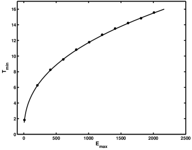
Figure 1: Comparison of the results of computer simulations of an ecosystem with theory. We consider a system with $100,000$ energy levels with $\varepsilon_{k}=k^{2/3}$, $k=1..100,000$, corresponding to $d=1/2$. We work with a constant $E_{max}$ (the figure shows the results for several values of $E_{max}$) and consider a dynamical process of birth and death. We have verified that the equilibrium distribution is independent of the initial condition. At any given time step, we make a list of all the individuals and the empty energy levels. One of the entries from the list is randomly picked for possible action with a probability proportional to the total number of entries in the list. Were an individual to be picked, it is killed with $50$% probability or reproduced (an additional individual of the same species is created) with $50$% probability provided the total energy of the system does not exceed $E_{max}$. When an empty energy level is picked, speciation occurs with $50$% probability and a new individual of that species is created provided again the energy of the system does not exceed $E_{max}$. With $50$% probability, no action is taken. This procedure is iterated until equilibrium is reached. The effective temperature of the ecosystem is defined as the imbalance between $E_{max}$ and the average energy of the system (Eq. (1)). The figure shows a plot of the effective temperature of the ecosystem deduced from the simulations. The circles denote the data averaged over a run of $10^{9}$ time steps with the last $500$ million used to compute the average temperature while the solid line is the theoretical prediction.

A strong hint that there is a link between the behaviors of the ecosystem at $T_{min}$ and the physical system of Bosons at the BEC transition is obtained by noting that both these situations are characterized by $\alpha=1$ or equivalently a zero basic cost ($\mu=0$) for the introduction of an individual or a particle into the system.

Let us set the value of $N_{max}$ equal to $N_{M}$, the average population in a system with $E_{max}=E_{M}$ and $N_{max}=\infty$, and consider the effect of varying the temperature. As in Bose condensation, one can identify (for $d>0$) a critical temperature, $T_{c}$, as the lowest temperature above which the first term on the rhs of Eq. (10) can be neglectedFeynman (1998). At $T_{c}$, $\langle N\rangle\approx N_{max}=N_{M}$ and $\alpha\approx 1$. Recall, however, that with only the energy ceiling, at $T=T_{min}$ the ecosystem was characterized by $\alpha=1$ and $\langle N\rangle=N_{M}$. This confirms that $T_{c}=T_{min}$. The macroscopic depletion of the community population, when $T<T_{min}$ is entirely akin to the macroscopic occupation of the ground state in BEC (Fig. 2).

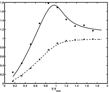
Figure 2: Phase transition in an ecosystem with $N_{max}=N_{M}=65$ and $d=1/2$. The dashed and solid curves are plots of theoretical predictions of $\frac{\langle N\rangle}{N_{M}}$ and $\frac{\partial\langle E\rangle}{\partial T}\frac{T_{min}}{E_{M}}$ respectively versus scaled temperature $T/T_{min}$, where $T_{min}=11.6$ and $E_{M}=1000$. The data points denote the results of simulations. $\partial\langle E\rangle/\partial T$ is a quantity analogous to the specific heat of a physical system and has the familiar $\lambda$ shape associated with the superfluid transition in liquid heliumFeynman (1998). It was obtained in the simulations as the derivative of the interpolated values of $\langle E\rangle$. The continuous phase transition is signaled by the peak in $\partial\langle E\rangle/\partial T$ (and the corresponding drop in $\langle N\rangle$) on lowering the temperature and occurs in the vicinity of the temperature $T_{min}$ (the transition temperature moves closer to $T_{min}$ as the system size increases).

When $T$ is larger than $T_{min}$, the energy resources are sufficient to maintain the maximum allowed population and $\langle N\rangle=N_{M}$. Physically, the state at $T_{min}$ corresponds to a maximally efficient use of the energy resources so that any decrease in $T$ below $T_{min}$ inevitably leads to a decrease of the population and the biodiversity in the community. The existence of this novel transition is quite general and is independent of specific counting rules such as the ones used in the classic examples of distinguishable and indistinguishable particlesFeynman (1998).

Our results suggest that ecosystems in equilibrium are organized in the vicinity of a novel critical point. Critical pointsWilson (1983) are generally characterized by large fluctuations and a slowing down of dynamics in their vicinity. It is an intriguing possibility that the ubiquity of power laws in ecologySchmidt-Nielsen (1984); Calder III (1984); McMahon and Bonner (1983); Peters (1983) may have some relationship to our findings here.