Information theory, multivariate dependence, and genetic network inference

Abstract

We define the concept of dependence among multiple variables using maximum entropy techniques and introduce a graphical notation to denote the dependencies. Direct inference of information theoretic quantities from data uncovers dependencies even in undersampled regimes when the joint probability distribution cannot be reliably estimated. The method is tested on synthetic data. We anticipate it to be useful for inference of genetic circuits and other biological signaling networks.

1 Two problems

One of the most active fields in quantitative biology is the inference of biological interaction networks (e. g., protein or genetic regulatory networks) from high throughput data such as expression microarrays [1]. In these problems, one measures (simultaneous or serial) values of expressions of genes under different conditions and treats them as samples from a joint probability distribution (PD). The goal is to infer the genetic network based on statistical dependencies in this PD.

This involves a conceptual and a technical problem. First, surprisingly, even now there is still no agreement on what the dependence, the interaction, is in a multivariate setting. Instead of a universal definition, standard statistical methods [3, 2] have produced a multitude of dependence concepts applicable in restricted contexts, such as normal noise, binary, bivariate, or metric data, etc. Of these, the notion of conditional (in)dependence in the form of Bayesian networks (BN) [1] has proved to be very useful in biological applications. However, it is insufficient to deal with regulatory loops, or to distinguish independent vs. cooperative regulation of a gene by others (see below). Further, statistical dependence is a symmetric property [4], while graphs of BNs are directed. Thus, to infer interaction networks, we must first carefully define what we mean by multivariate statistical dependence.

The goal is to partition the overall statistical dependence, that is, the deviation of the joint PD (JPD) from the product of its marginals, into contributions from interactions of different kinds (among pairs of variables, triplets, etc.), and, better yet, from specific combinations of variables within a kind. Many ideas have been suggested [2, 5, 6], but the most natural approach is to quantify the new knowledge that comes from looking at a complete JPD vs. its approximations under various independence assumptions. For example, in contingency tables analysis, one studies deviations of the number of observed counts from their expectations under such assumptions [7, 8, 9, 11, 10]. Such discussion is limited to categorical data and, importantly, confounds the definition of dependence with sampling issues. Information theory [12, 13] provides tools to treat continuous and categorical data uniformly [15, 14] and to generalizes bivariate dependence measures to multivariate cases based on distributions rather than counts. However, some suggested information theoretic measures [19, 20, 26, 23, 24, 25, 21, 22, 16, 18, 17] are not necessarily nonnegative, or involve averaging logarithms of fractional powers of PDs. Thus they cannot characterize sizes of typical sets and have not become universally accepted. Instead, one notices that the maximum entropy (MaxEnt) distributions [27, 28] consistent with some marginals of the JPD introduce no statistical interactions beyond those in the said marginals. Thus the JPD can be compared to its MaxEnt approximations to separate dependencies included in the low order statistics from those not present in them [23, 4]. This approach completely characterizes multivariate interactions for binary [30, 29] or exponential [31] distributions. In general, it led to a definition of connected interactions of a given order, that is, the interactions that need, at least, the full set of marginals of this order to be captured [32]. However, there has been no successful attempt of defining dependence among variables, that is, localizing (connected) interaction to particular covariates.

The second, technical, problem emerges if we agree on the measures of dependence. The usual approach then is to use the experimental data to infer the JPD in question and evaluate these measures for it. Unfortunately, the distributions may be severely undersampled. To fight this, the field has focused on a simplistic approach [34, 33]: (a) assume some dependence structure; (b) regularize the JPD consistently with it and learn it from the data; (c) evaluate the quality of fit; (d) repeat until the dependence structure with the best fit is found. Validity of such analysis is sensitive to the choice of the regularization, and a bad choice may lead to misestimation of dependencies. As a rule, inferring a complicated object (the JPD) in order to only find its simple property (the dependencies) is not a good idea [35], and a direct estimation of dependencies without learning the JPD is preferred.

From Shannon’s work [12] and its later developments [4, 32] we know that we have to look at information theoretic quantities to measure dependence. Many of these are differences of (marginal, conditional) entropies of the JPD. While earlier works [19, 4] relied on good sampling, we now know that, at least under some conditions, entropy may be estimated reliably even when inferences about details of the underlying PD are impossible. Thus the direct estimation of dependencies has a chance even for undersampled problems.

In this paper we deal with both the conceptual and the technical problem. First, expanding on [4, 32] (see also [39] for axiomatization), we systematically characterize dependencies among variables. Second, we apply direct entropy estimation methods to undersampled synthetic data to show that interactions can be uncovered even in that regime.

2 Definitions

Suppose we have a network of $M$ covariates $X_{i}$, $i=1,\dots,M$, (called nodes, expressions, or genes) that take random values $x_{i}$ respectively with the joint probability $P({\bf x})$. The total statistical dependence among the variables is given by their multiinformation, that is, the Kullback–Leibler divergence between the JPD and the product of the marginals [32, 39],

$$I[P]:=\sum_{\{x_{i}\}}P({\bf x})\log_{2}\frac{P({\bf x})}{\prod_{i}P(x_{i})}=\left<\log_{2}\frac{P({\bf x})}{\prod_{i}P(x_{i})}\right>=\sum_{i}S[X_{i}]-S[{\bf X}]\,,$$ (1)

where $\sum$’s represent summations for discrete and integration for continuous variables respectively, and $S[X]:=-\sum P(x)\log_{2}P(x)$ is the entropy of $P(x)$.

Following [32], we localize these bits of dependence to statistical interactions of different orders. If all $m$-way marginals, $P(x_{i_{1}},x_{i_{2}},\dots,x_{i_{m}})$, are known, then one finds an approximation to the JPD that respects the marginals, but makes no additional assumptions about the JPD. This is given by the MaxEnt, or minimum multiinformation, problem [27, 4, 32]:

$$P^{(m)}:=\arg\max_{P^{\prime},\{\lambda\}}\bigg{\{}S[P^{\prime}]-\sum_{i_{1}<\cdots<i_{m}}^{M}\sum_{x_{i_{1}}\dots x_{i_{m}}}\lambda_{i_{1}\dots i_{m}}(P^{\prime}_{i_{1}\dots i_{m}}-P_{i_{1}\dots i_{m}})\bigg{\}},$$ (2)

where $\lambda$’s are the Lagrange multipliers enforcing the marginal constraints; different $\lambda$’s are distinguished by their arguments. The arguments of all functions are listed in their lower indices, e. g., $P_{1}:=P(x_{1})$. No indices means dependence on all variables, while ${\not i}$ on all, but $X_{i}$. Further, a distribution with lower indices is a marginal, e. g., $P_{12}:=\sum_{\not x_{1}\not x_{2}}P$.

A solution of any MaxEnt problem with marginal constraints has a form of a product of terms depending on the constrained variables [40]. In particular, for Eq. (2),

$$P^{(m)} = \prod_{i_{1}<\cdots<i_{m}}f_{i_{1}\dots i_{m}},\;\;f\geq 0,$$ (3)

$$P_{i_{1}\dots i_{m}}^{(m)} = P_{i_{1}\dots i_{m}},\;\;\forall\{i_{1},\dots,i_{m}\},$$ (4)

where $f$’s, again distinguished by their arguments, are to be found from the constraints. Note the Boltzmann machine or Markov network structure of this MaxEnt distribution [41, 1]. In general, no analytical solution for $f$’s exists. However, an algorithm called the iterative proportional fitting procedure (IPFP) [42], which iteratively adjusts a trial solution to satisfy each of the constraints in turn, converges to the true solution [40].

Finding $P^{(m)}$ and $P^{(m-1)}$ defines connected information [32]

$$I^{(m)}[P] := \left<\log_{2}\frac{P^{(m)}}{P^{(m-1)}}\right>\,;$$ (5)

$$I[P] = \sum_{m=2}^{M}I^{(m)}[P]\,,$$ (6)

which measures the amount of statistical interactions accounted for by $m$-way, but not by $m-1$-way marginals. This is similar to connected correlation functions or cumulants.

In the same spirit, to determine if a particular $m$–way interaction contributes to $I$, we may check if fixing the corresponding $P_{i_{1}\dots i_{m}}$ recovers any dependencies not already contained in a reference MaxEnt distribution $Q^{*(i_{1}\dots i_{m})}$ constrained by some other marginals. That is, we define the interaction multiinformation

$$\Delta^{(i_{1}\dots i_{m})}:=\left<\log_{2}\frac{Q^{(i_{1}\dots i_{m})}}{Q^{*(i_{1}\dots i_{m})}}\right>=I^{(i_{1}\dots i_{m})}-I^{*(i_{1}\dots i_{m})},$$ (7)

where $Q^{(\cdot)}$ is the interaction MaxEnt distribution satisfying all constraints of $Q^{*(\cdot)}$ and additionally having $Q^{(\cdot)}_{i_{1}\dots i_{m}}=P_{i_{1}\dots i_{m}}$. $I^{(\cdot)}$ and $I^{*(\cdot)}$ are multiinformations of $Q^{(\cdot)}$ and $Q^{*(\cdot)}$ respectively. By positivity of the Kullback–Leibler divergence, $\Delta^{(\cdot)}\geq 0$. Thus if $\Delta^{(\cdot)}>0$, accounting for the marginal $P_{i_{1}\dots i_{m}}$ recovers more multiinformation, and we say that the corresponding interaction or dependence is present with respect to $Q^{*(\cdot)}$.

The problem is that $\Delta^{(\cdot)}$ depends on the choice of $Q^{*(\cdot)}$. To test the null hypothesis of no dependencies, we must select the reference $Q^{*(\cdot)}$ that minimizes the interaction information. This guarantees that interactions are accepted only if they cannot be reduced to some other statistical dependencies in the network. According to Thm. 1 (see Appendix), such reference distribution is given by

$$Q^{*(i_{1}\dots i_{m})} = f_{{\not i}_{1}}\cdots f_{{\not i}_{m}},\;\;f\geq 0$$ (8)

$$Q^{*(i_{i}\dots i_{m})}_{{\not i}_{k}} = P_{{\not i}_{k}},\;\forall k=1\dots m.$$ (9)

This $Q^{*(\cdot)}$ preserves all marginals of the original JPD except those that involve all $m$ co–variates being examined for an interaction. This is similar to the Type III Sum of Squares ANOVA for testing significance of predictors. In fact, since $D_{\rm KL}$ is equal to $\chi^{2}$ asymptotically, the similarity is not accidental. Dependence defined by this choice of $Q^{*(\cdot)}$ is a generalization of the conditional dependence with the rest of the network as a condition.

The interaction PD, which additionally preserves the joint statistics of $X_{i_{1}},\dots,X_{i_{m}}$, but nothing extra, is

$$Q^{(i_{1}\dots i_{m})} = f_{{\not i}_{1}}\cdots f_{{\not i}_{m}}f_{i_{1}\dots i_{m}},\;\;f\geq 0$$ (10)

$$Q^{(i_{i}\dots i_{m})}_{{\not i}_{k}} = P_{{\not i}_{k}},\;\forall k=1\dots m,$$ (11)

$$Q^{(i_{i}\dots i_{m})}_{i_{1}\dots i_{m}} = P_{i_{1}\dots i_{m}}.$$ (12)

Using such $Q$ and $Q^{*}$ in Eq. (7) defines irreducible $m$–way interactions (dependencies) among particular $m$ variables. We denote these dependencies graphically by edges coming from the variables and meeting at an $m$–edge vertex, see Fig. 1. This graphical notation generalizes BNs and [32], were the only goal was to denote $m$–way interactions among all combinations of co-variates simultaneously.

3 Examples and properties

We consider a few examples for $M=3$ (larger $M$ is analyzed similarly). First, a regulatory cascade, or a Markov chain: $X_{1}\to X_{2}\to X_{3}$, $P(x_{1},x_{2},x_{3})=P(x_{1})P(x_{2}|x_{1})P(x_{3}|x_{2})$. Looking for $X_{1}X_{2}$ dependence, we have $I^{*(12)}=I[X_{1},X_{3}]+I[X_{2},X_{3}]\leq I^{(12)}=I[X_{1},X_{2}]+I[X_{2},X_{3}]$, where the inequality is due to the information processing inequality, and the bound is reached only in special cases. Thus $X_{1}$, $X_{2}$ are (generically) dependent. Similarly, $X_{2}$, $X_{3}$ are dependent; but $\Delta^{*(13)}=0$, and $X_{1}$, $X_{3}$ are not (even though their marginal mutual information, induced by other interactions, is not zero). Checking for the triplet interactions, we find $I^{*(123)}=I[X_{1},X_{2}]+I[X_{2},X_{3}]=I^{(123)}$, thus no such dependencies are present. If now instead $X_{2}$ regulates $X_{1}$ and $X_{3}$, one sees that the dependence structure is the same. Both networks correspond to the graph in Fig. 1(a).

Figure 1: Examples of dependencies for $M=3$.

A more interesting case is when $X_{1}$, $X_{3}$ regulate $X_{2}$ jointly. Here many possibilities exist, not all of them realizable in terms of BN modeling. First, consider independent regulation: to predict $X_{2}$, one does not need to know the values of $X_{1}$ and $X_{3}$ simultaneously, $P(x_{2}|x_{1},x_{3})=f_{12}f_{23}$, e. g., $P(x_{2}|x_{1},x_{3})\propto\exp\left[-a(x_{2}-x_{1})^{2}-b(x_{2}-x_{3})^{2}\right]$ (this corresponds to OR and AND gates [32], to the Lac–repressor [43], and to all regulatory models based on independent binding of transcription factors to the DNA [44]). If $P_{13}=P_{1}P_{3}$, then the dependency structure is again as in Fig. 1(a). If in addition there is a regulation $X_{1}\to X_{3}$, so that $P_{13}\neq P_{1}P_{3}$, then $\Delta^{(13)}=D_{\rm KL}[P||Q^{*(13)}]\geq 0$, and $\Delta^{(123)}=0$. The dependency graph now has a loop in it, as in Fig. 1(b).

Further, in the joint regulation case one may consider a nonfactorizable $P_{123}$ with all pairwise marginals factorizable. An example is the XOR gate [32, 43] (we were unable to construct an explicit, normalized example for continuous variables). In this case, $\forall i,j,\,I^{(ij)}=0$. $\Delta^{(123)}>0$, and the dependence structure is as in Fig. 1(c). Combinations of two- and three–way dependencies are also possible [Fig. 1(d–f), etc.]; for example, an explicit construction for the case (e) is $P_{123}\propto\exp[-a(x_{2}-x_{3}x_{1})^{2}]P_{1}P_{3}$. Such higher order dependencies are uncommon in physics, which usually deals with low order interactions among many variables (for example, the Hamiltonian for a spin system is $H=-\sum_{ij}J_{ij}\sigma_{i}\sigma_{j}$; thus the JPD of spins has no interactions of order $m>2$). In contrast, combinatorial regulation in genetics requires considering higher order models.

While such detailed classification is overwhelming for large $M$, some general statements may be proven for our choice of $Q^{*},Q$. In particular, similar to Eq. (6), we have

$$I[P]\geq\sum_{\mbox{all subsets of $\{X_{i}\}$}}\Delta^{(\mbox{subset})}.$$ (13)

Here the inequality is the result of our conservative approach to identification of dependencies. To prove it, we order all $m$–way dependencies in an arbitrary way. We then evaluate the interaction information for the first dependency with $P^{(m-1)}$ as the reference distribution, and take the interaction PD for each dependency as the reference PD for the next one. Summing all $m$–way interactions gives $I^{(m)}$, and summing over $m$ results in $I[P]$ [cf. Eq. (6)]. On the other hand, according to Thm. 1, $\Delta^{(\cdot)}$ evaluated this way is not smaller than the one with the references Eq. (8). This proves the above inequality.

For $M=3$, an interesting illustration of Eq. (13) is $P_{123}=P_{1}\,\delta(x_{1}-x_{2})\,\delta(x_{2}-x_{3})$. We correctly identify all interactions as reducible (all $\Delta$’s are zero). However, to account for the multiinformation in this PD, (any) two pairwise interactions must be invoked. The degeneracy is lifted if, for example, noise breaks the symmetry among $X$’s.

Finally, we note another interesting property of our definition. For continuous $x_{i}$, the presence of interactions does not depend on (nonsingular) reparameterizations of variables that do not mix them, $x_{i}\to y_{i}(x_{i})$ (see [2] for a discussion of importance of this):

$$\Delta^{(\cdot)}[P(x_{1},\dots,x_{M})]=\Delta^{(\cdot)}[P(y_{1},\dots,y_{M})].$$ (14)

This is true since such transformations do not change factorization properties of the MaxEnt distributions, and the Jacobians cancel in the definition of $\Delta^{(\cdot)}$. Note that, while the definition is reparameterization invariant, inference of distributions cannot be done in a covariant way [45]. The invariance vanishes if instead of $P$ only a sample from it is given.

4 Inferring networks from data

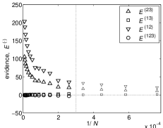
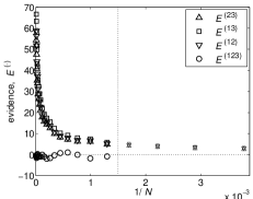
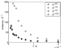
(a) (b) (f)

Figure 2: Inferring regulatory networks from $N$ samples. We used the NSB [36] method to estimate the entropies (with error bars) of the JPD and its marginals directly. The method does not work for $Q^{*(123)}$. Thus IPFP was applied to the counts and the entropy $S^{*(123)}$ of the solution was evaluated and extrapolated for $1/N\to 0$ following Strong et al. [46] to account for the sample size dependent bias. The statistical error for each sample size $N$ was determined by bootstrapping, and the resulting extrapolation error was used for $\delta S^{*(123)}$. This approach works since the MaxEnt constraints, like those in Eq. (2), are linear in the unknown JPD $P$, making the biases of $S[P]$ and $S^{*(123)}$ behave similarly. Finally, $\Delta^{(\cdot)}$ were calculated as the differences of the appropriate entropies, and $\delta^{2}\Delta^{(\cdot)}$ as the sums of squares of the entropy errors. (a) Network in Fig.1(a). To the left of the vertical dotted line, $N\approx 3000\gtrsim 2^{S^{*(123)}}\ll K\approx 125000$, the sample size corrections are reliable, and all entropies are known well. There is evidence only for $X_{1}X_{2}$ and $X_{2}X_{3}$ interactions, just as it should be. For smaller $N$, the method of Strong et al. fails, but NSB works until $N\sim 2^{1/2S[P]}\approx 60$. For pairwise interactions, we may replace $S^{*(123)}$ by $S[P]$ (denoted by smaller markers on the plot) and, since $E^{(13)}$ stays zero nonetheless, and $I[X_{1},X_{2}]+I[X_{2},X_{3}]=I[P]$, we still recover the interactions correctly. (b) Network in Fig. 1(b). Again, to the left of the line, $N\approx 700\gtrsim 2^{S^{*(123)}}$, all entropies are determined reliably, and there is evidence for all three pairwise interaction, but not for the triplet interaction. To the right of the line, NSB still works, but now we cannot disentangle the loop from the three–way dependence without estimating $S^{*(123)}$. (c) Network in Fig. 1(f). Only the regime $N\gtrsim 2^{S^{*(123)}}\approx 5000$ is shown. The evidence for all three pairwise interactions and for the triplet interaction is barely significant for small $N$ but grows fast.

A big advantage of our definition of statistical dependencies in terms of the MaxEnt approximations is that it can be applied even when the underlying PDs are undersampled, and the corresponding factorizations cannot be readily observed. For $K$, the cardinality of a variable, larger than the number of samples, $N$, we cannot estimate the PDs reliably, but entropic quantities, and, therefore, the interactions are inferable (some progress is possible even for $N\sim\sqrt{K}$). To show this, we used Dirichlet priors [36] to generate random probability distributions with different interaction structures, $M=3$, and with marginal cardinalities $K_{i}\approx 50$. We generated random samples of different sizes, $N=50\dots 125000$ from these distributions and tested the quality of inference of the dependencies as a function of $N$. To measure it, we used the evidence for some dependency, $E^{(\cdot)}:=\Delta^{(\cdot)}/\delta\Delta^{(\cdot)}$, where $\delta\Delta^{(\cdot)}$ is the statistical error of the interaction multiinformation. If $E^{(\cdot)}$ is large, the dependency is present. According to Fig. 2, proper recovery is possible for $N\ll K=K_{1}K_{2}K_{3}$ with few assumptions about the form of the PDs.

With modern entropy estimation techniques [36], our approach will work even for severely undersampled JPD. The bottleneck is the estimation of the maximum entropy consistent with the marginals, which currently requires substantial sampling of the marginals [46]. This is encouraging, since they may be well sampled when the JPD is not. However, it is still essential to develop techniques to infer maximum entropies directly. Further, the interaction information is the difference of entropies. It may be small when its error, which is a quadratic sum of the entropy errors, is large. This leads to uncertainties about dependencies even for reliably estimated entropies, see the small $N$ region in Fig. 2(c). Therefore, a method that directly estimates $\Delta$ will be preferred over another entropy–based technique. Finally, as in Fig. 1(a), variables may have nonzero mutual (or higher order) information and no direct interactions. Thus, if $X_{2}$ was unobserved, we would have inferred a dependence between $X_{1}$ and $X_{3}$. Similarly, spurious higher order interactions may also emerge. Our method, just like most other assumption–free methods, may fail for hidden variables.

For genomic applications, the number of different expression measurements is $N\lesssim 100$, and it is not nearly enough to estimate $\Delta$’s and to infer the full interaction network of, say, $M\approx 6000$ genes in a yeast. However, for ternary discretization of expressions, with the Strong et al. entropy estimation, one will not find significant evidence for $I^{(m)}$ beyond $m^{*}\sim\log_{3}N\approx 4$ (or somewhat larger if PDs are far from being uniform). Then one can replace $P$ by $P^{(m^{*})}$ in Eq. (8) and study interactions up to the order $m^{*}$ with respect to this JPD. It is possible that most interactions in genomes are of such low orders. Additionally, if methods like NSB [36] are developed for MaxEnt analysis, one should be able to push for $m^{*}\sim 2\log_{3}N\approx 8$, and this is the primary goal of our future work.

In summary, we have formalized the concept of multivariate dependence, suggested a way to infer dependencies from data, tested the suggestion on undersampled synthetic examples, and hinted at possible applications to genomic research.

Appendix

Theorem 1

Let $\{C\}$ be a set of noncontradictory marginal constraints and $Q^{{C}}$ be the MaxEnt distributions satisfying these constraints. Further, let $C_{0}$ and $C_{1}$ be additional constraints (possibly included in $\{C\}$), and $Q^{C0}$, $Q^{C1}$, and $Q^{C01}$ be the MaxEnt PDs satisfying $\{C\}\cup C_{0}$, $\{C\}\cup C_{1}$, and $\{C\}\cup C_{0}\cup C_{1}$ respectively. Then

$$\left<\log_{2}\frac{Q^{C01}}{Q^{C0}}\right>\leq\left<\log_{2}\frac{Q^{C1}}{Q^{C}}\right>,$$ (15)

where the averaging is performed over $Q^{C01}$.

Intuitively, this says that the interaction multiinformations depend on the order in which the interactions are considered. Dependency bits will be accounted for by the first marginal able to explain them, attributing less bits to later constraints. At present, this theorem has been extensively tested by numerical simulations, but still remains a conjecture.

References

- [1] N. Friedman: Science 303 (2004) 799
- [2] H. Joe: Multivariate models and dependence concepts: Chapman & Hall, Boca Raton (1997)
- [3] A. Agresti: Categorical Data Analysis: Wiley, New York (1990)
- [4] H. H. Ku, S. Kullback: J. Res. Natl. Bur. Stand. (Math. Sci) 72B (1968) 159
- [5] M. Schlather, J. Tawn: Biometrika 90 (2003) 139
- [6] I. Goodman, D. Johnson: In: 2004 Int. Conf. Acoustics, Speech, and Signal Processing (ICASSP). IEEE (2004)
- [7] H. O. Lancaster: J. Roy. Stat. Soc. Ser. B (Methodol.) 13 (1951) 242
- [8] S. N. Roy, M. A. Kastenbaum: Ann. Math. Stat. 27 (1956) 749
- [9] J. N. Darroch: J. Roy. Stat. Soc. Ser. B (Methodol.) 24 (1962) 251
- [10] F. Mosteller: J. Amer. Stat. Assoc. 63 (1968) 1
- [11] B. N. Lewis: J. Roy. Stat. Soc. Ser. A (General) 125 (1962) 88
- [12] C. E. Shannon, W. Weaver: The Mathematical Theory of Communication: University of Illinois Press, Urbana (1949)
- [13] T. Cover, J. Thomas: Elements of information theory: John Wiley & Sons, New York, 2nd edn. (1991)
- [14] S. Kullback: Ann. Math. Stat. 39 (1968) 1236
- [15] C. T. Ireland, S. Kullback: Biometrika 55 (1968) 179
- [16] G. Chechick, et al.: In: Adv. Neural Inf. Proc. Syst. 14, eds. T. Dietterich, S. Becker, Z. Ghahramani, Cambridge, MA (2002). MIT Press
- [17] E. Schneidman, W. Bialek, M. J. Berry: J. Neurosci 23 (2003) 11539
- [18] M. Bezzi, M. E. Diamond, A. Treves: J. Comp. Neurosci. 12 (2002) 165
- [19] W. McGill: IRE Trans. Inf. Thy. 4 (1954) 93
- [20] W. R. Garner, W. J. McGill: Psychometrika 21 (1956) 219
- [21] H. Matsuda: Phys. Rev. E 62 (2000) 3096
- [22] A. J. Bell: Co-information lattice: Tech. Rep. RNI-TR-02-1, Redwood Neurosci. Inst. (2002)
- [23] I. J. Good: Ann. Math. Stat. 34 (1973) 911
- [24] T. S. Han: Information and Control 36 (1978) 133
- [25] M. Studeny, J. Vejnarova: In: Learning in Graphical Models, ed. M. I. Jordan, pp. 261–298. Kluwer, Dordrecht (1998)
- [26] S. Watanabe: IBM J. of Research and Development 4 (1960) 66
- [27] E. T. Jaynes: Phys. Rev. 106 (1957) 620
- [28] P. M. Lewis: Information and Control 2 (1959) 214
- [29] L. Martignon, et al.: Neural Comput. 12 (2000) 2621
- [30] E. Soofi: J. Amer. Stat. Assoc. 87 (1992) 812
- [31] S. Amari: IEEE Trans. Inf. Thy. 47 (2001) 1701
- [32] E. Schneidman, S. Still, M. J. Berry, W. Bialek: Phys. Rev. Lett. 91 (2003) 238701
- [33] C. Wiggins, I. Nemenman: Experim. Mech. 43 (2003) 361
- [34] Y. Barash, N. Friedman: Context–specific Bayesian clustering for gene expression data: Tech. Rep. 2002-05, Hebrew University, CS, Leibnitz center (2002)
- [35] V. Vapnik: Statistical learning theory: John Wiley & Sons, New York (1998)
- [36] I. Nemenman, F. Shafee, W. Bialek: In: Advances in Neural Information Processing Systems 14, eds. T. G. Dietterich, S. Becker, Z. Ghahramani, Cambridge, MA (2002). MIT Press
- [37] I. Nemenman, W. Bialek, R. de Ruyter van Steveninck: Phys. Rev. E 69 (2004) 056111
- [38] J. Beirlant, E. Dudewicz, L. Gyorfi, E. van der Meulen: Int. J. Math. Stat. Sci. 6 (1997) 17
- [39] I. Nemenman, N. Tishby: In preparation
- [40] I. Csiszar: Ann. Probab. 3 (1975) 146
- [41] G. Hinton, T. Sejnowski: In: Parallel Distributed Processing, eds. D. Rumelhart, J. McClelland, vol. 1, chap. 7 pp. 282–317. MIT Press, Cambridge, MA (1986)
- [42] W. E. Deming, F. S. Stephan: Ann. Math. Stat. 11 (1940) 427
- [43] N. Buchler, U. Gerland, T. Hwa: Proc. Natl. Acad. Sci. USA 100 (2003) 5136
- [44] H. Bussemaker, E. Siggia, H. Li: Nature Genetics 27 (2001) 167
- [45] T. Holy, I. Nemenman: Tech. Rep. NSF-KITP-03-123, KITP, UCSB (2002)
- [46] S. P. Strong, R. Koberle, R. R. de Ruyter van Steveninck, W. Bialek: Phys. Rev. Lett. 80 (1998) 197