Performance of networks of artificial neurons: the role of clustering

Abstract

The performance of the Hopfield neural network model is numerically studied on various complex networks, such as the Watts-Strogatz network, the Barabási-Albert network, and the neuronal network of the C. elegans. Through the use of a systematic way of controlling the clustering coefficient, with the degree of each neuron kept unchanged, we find that the networks with the lower clustering exhibit much better performance. The results are discussed in the practical viewpoint of application, and the biological implications are also suggested.

Recently, researches related with complex networks have been broadening territory beyond individual disciplines. Starting from pioneering works of modeling complex networks WS ; BA , the essential network concepts have been successfully applied to various systems covering biological networks, food webs, Internet, e-mail network, and so on ref:network . In parallel to the studies of structural properties of complex networks, there have also been strong interest in dynamic systems defined on networks. For examples, non-Hamiltonian dynamic models such as epidemic spread epidemic , cascading failures cascading , synchronization synch ; smallmembrane , the sandpile sand , and the prisoner’s dilemma game pd , as well as equilibrium statistical physics models such as the Ising ising and the $XY$ smallXY models have been investigated.

The network of neurons in biological organisms also takes the form of complex networks ref:network ; realneuronnet ; neuroanatomy ; karbowski . While the C. elegans WS ; ref:network ; cherniak and the in vitro realneuronnet neuronal networks have the high level of clustering, the small characteristic path length, and the degree distribution far from scale-free in common, the functional network of human brains dante has recently been revealed to be scale-free. Motivated by the neurons connected by synaptic couplings in biological organisms, simple mathematical models of artificial neurons have been suggested hopfieldreview . One of the practical applications of such an artificial neural network can be found in the Hopfield model hopfieldreview , which is used frequently in the pattern recognition. Very recently, there have been studies of the Hopfield model of neurons put on the structure of complex networks neuronnet ; costa , with major focus on how the topology, the degree distribution in particular, of a network affects the computational performance of the Hopfield model. Also in the neuroscience, recent investigations have revealed the close interrelationship between the brain activity and the underlying neuroanatomy neuroanatomy .

Table 1: Performance of Hopfield model on networks. All networks are of the same size $N=280$ and the average degree $\langle k\rangle\approx 14$. The neuronal network of the worm C. elegans, the Barabási-Albert (BA) network, and the Watts-Strogatz (WS) networks at the rewiring probabilities $P=0.0,0.1$, and 1.0 are used. Both the overlap $m$ and the input-output ratio $R$, measuring the performance of the network, increase as the clustering coefficient $\gamma$ is decreased. The maximum degree $k_{\rm max}$ is also shown to give some rough estimation of the broadness of the degree distribution.

Network	$k_{\rm max}$	$\gamma$	$m$	$R$
WS($P=0.0$)	14	0.69	0.689	0.603
WS($P=0.1$)	17	0.50	0.743	0.623
C. elegans	77	0.28	0.798	0.642
BA	67	0.11	0.838	0.656
WS($P=1.0$)	22	0.05	0.881	0.672

Table 1 summarizes the clustering coefficients (see Ref. WS, for the definition) and the performance of the Hopfield model on various network structures fullpaper (see below for details). The difference in the performance, measured by the overlap $m$ between the neuron state and the stored pattern, has been previously attributed to the distinct network topology, or the degree distribution more specifically neuronnet . Examining Table 1 in more detail, one can easily recognize the systematic dependence of the network performance on the clustering property: As the clustering becomes weaker, the performance is enhanced monotonically. The performance detected by the ratio $R$ (the last column in Table. 1, see Ref. forrest, ) of the number of correctly recalled bits to the number of synaptic couplings again shows the same behavior.

We in this work study the performance of the Hopfield model on various network structures with focus on the role of the clustering. We extend the edge exchange method in Ref. sneppen, and suggest a systematic way to control the clustering coefficient of a given network without changing the degree of each vertex. A set of networks with the identical degree distribution but with various clustering coefficients are generated and then used as the underlying network structures for the numerical simulations of the Hopfield model. Clearly revealed is that the computational performance depends much more strongly on the clustering property than on the degree distribution.

We begin with a brief review of the edge exchange method, recently suggested by Maslov and Sneppen in Ref. sneppen, . Two edges, one connecting vertices A and B, and the other C and D, are randomly chosen [Fig. 1(a)]. Each vertex changes its partner and the original edges A-B and C-D are altered to A-D and B-C as shown in Fig. 1(b). The important property of the above edge exchange is that this process does not change the degree of each vertex. A blind repetitions of the above edge exchanges have been shown to destroy all degree-degree correlations sneppen ; dante .

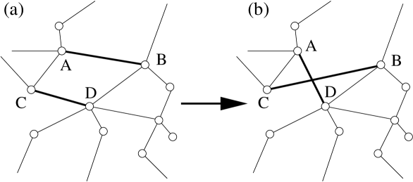
Figure 1: Exchange of two edges: Two edges [A-B and C-D in (a)] are randomly picked and then rewired to have different end vertices [ A-D and C-B as in (b)]. The edge exchange keeps the degree of each vertex unchanged.

Based on the above edge exchange method, we in the present paper introduce an additional acceptance stage: The edge exchange trial is accepted only when the new network configuration has higher (or lower) clustering coefficient. This is identical to the standard Monte Carlo (MC) simulation at zero temperature ($T$) with the Hamiltonian $H$ set to $H=-\sum_{v}\gamma_{v}$ (or $H=\sum_{v}\gamma_{v}$), where $\gamma_{v}$ is the clustering coefficient of the vertex $v$ WS . In addition, we also apply the standard MC scheme to the above Hamiltonian at finite temperatures. In either way, one can control the clustering coefficient of a given network with the degree of each vertex kept fixed.

We use various network structures as underlying networks of the Hopfield model. Since the real neuronal network of C. elegans has $N=280$ vertices and the average degree $\langle k\rangle\approx 14$, we generate various model networks of the size $N=280$ such as Barabási-Albert (BA) network with $M_{0}=M=7$ (starting from $M_{0}$ vertices, one vertex with $M$ edges is added at each step in the BA model BA ), and the Watts-Strogatz (WS) networks with the connection range $r=7$ at the rewiring probabilities $P=0$ (corresponding to a regular local one-dimensional network), $P=0.1$ (well inside in the small-world regime WS ), and $P=1.0$ (corresponding to a fully random network). All the networks have different topologies in the sense that each has its own unique degree distribution. After the original networks are built, we decrease or increase the clustering coefficients through the use of the above zero-temperature MC method. Once the target value of the clustering coefficient is reached, the current network structure is frozen and then used as an underlying network structure for the Hopfield model. We also perform MC at finite temperatures with the Hamiltonian $H=-\sum_{v}\gamma_{v}$ to generate networks at a given $T$ for comparisons.

In the Hopfield model of a neural network hopfieldreview , a neuron at the site $i$ can have two states, firing ($\sigma_{i}=1$) or not firing ($\sigma_{i}=-1$). The neuron state $\sigma_{i}(t)$ at time $t$ is determined from the configuration of other neurons at $t-1$ according to

$$\sigma_{i}(t)={\rm sgn}\left(\sum_{j}\Lambda_{ij}W_{ij}\sigma_{j}(t-1)\right),$$ (1)

where $W_{ij}$ is the strength of the synaptic coupling between neurons $i$ and $j$, and $\Lambda_{ij}(=0,1)$ describes the connection structure of the neural network. For example, in the original version of the Hopfield neural network the couplings are of the mean-field type and thus $\Lambda_{ij}=1$ is taken for any pair $(i,j)$ of two neurons. In the standard graph theory, $\Lambda_{ij}$ is simply the $(ij)$-component of the so-called adjacency matrix, i.e., $\Lambda_{ij}=1$ if two vertices $i$ and $j$ are connected while $\Lambda_{ij}=0$ otherwise. For simplicity, we in this work consider only undirected networks and accordingly $\Lambda$ is a symmetric matrix. Recently, Hopfield model on the asymmetric directed BA network has been studied costa . According to Eq. (1), the firing of neighbor neurons connected to the $i$th neuron via excitatory synaptic couplings ($W_{ij}>0$) leads to the firing of $i$th neuron at next time step, while inhibitory couplings ($W_{ij}<0$) inhibits the firing of $i$th neuron.

For the task of the recognition of $p$ stored patterns, the synaptic coupling strength $W_{ij}$ is usually given by the Hebbian learning rule:

$$W_{ij}=\sum_{\mu=1}^{p}\xi_{i}^{\mu}\xi_{j}^{\mu},$$ (2)

where $\xi_{i}^{\mu}$ is the $i$th component of the $\mu$th stored pattern vector and is quenched random variable taking values $1$ and $-1$ with equal probability. In this work, we present results only for $p=5$ (we also tried $p=10$ and $20$ only to find insignificant qualitative differences). The initial neuron state configuration $\{\sigma_{i}(t=0)\}$ is produced from the one of the pattern vectors, say the $\nu$th pattern, with 20% error. In other words, $\sigma_{i}(0)=\xi_{i}^{\nu}$ for 80% of the neurons, while the other 20% has the reversed bit $\sigma_{i}(0)=-\xi_{i}^{\nu}$. As the neuron configuration evolves in time by Eq. (1), the overlap $m$ defined by

$$m(t)\equiv\frac{1}{N}\sum_{i}\sigma_{i}(t)\xi_{i}^{\nu}$$ (3)

is measured as a function of time. The complete recognition of the pattern $\nu$ gives $m=1$, which corresponds to the null Hamming distance $d(t)\equiv(1/N)\sum(\sigma_{i}(t)-\xi_{i}^{\nu})^{2}=2-2m(t)$. We also measure the input-output ratio $R$ of the correctly recalled pixels to the number of synaptic couplings, which is written as $R=(1+m)p/\langle k\rangle$ forrest ; fullpaper . The asynchronous dynamics, in which a neuron is chosen at random at each time step, is used throughout the present work. After sufficiently long runs of dynamic evolution up to $t=2000$, where the one time unit corresponds to the one whole sweep of all neurons, the last 200 time steps are used to make the time average of $m(t)$, and disorder averages over 1000 different pattern realizations are performed.

Figure 2: Efficiency of the Hopfield neural network on the C. elegans neuronal network, Barabási-Albert (BA) network, and Watts-Strogatz (WS) network at the rewiring probabilities $P=0,0.1$, and $1.0$. The overlap $m$ between the stored pattern and the neuron state measures the performance of each network and is plotted as a function of the clustering coefficient $\gamma\equiv(\sum\gamma_{v})/N$. The big filled circles are for the original networks before the edge exchange MC is applied (see text for details). It should be noted that at all points on each curve, not only the degree distribution but also the actual degree of each neuron is exactly identical. Performance of each network monotonically decreases as the clustering becomes stronger.

Figure 2 is the main result of the present paper. For each network, we start from the original network structure (denoted by the big filled circle on each curve), and increase (or decrease) the clustering coefficient by using the edge exchange zero-temperature MC method described above. Once the target value of the clustering coefficient ($\gamma=0.0,0.05,0.10,0.15,\cdots)$ is achieved the network structure is saved and used for the Hopfield model simulations. We repeat this procedure for 5-10 times to make an average over network structures. We also present the result obtained for finite-temperature MC method in Fig. 3; We start from the original network at sufficiently high temperature $T=1$ and use the standard Metropolis algorithm applied for $H=-\sum_{v}\gamma_{v}$. At each $T$, we equilibrate the network for $10^{4}$ MC steps and perform the Hopfield model dynamic simulation. The temperature is then decreased slowly to make equilibration at each $T$ more efficient. It is to be noted that we have introduced the finite temperature only when we generate networks by edge-exchange; the time evolution of neuron states in Eq. (1) is still deterministic.

The most important conclusion one can make out of Figs. 2 and 3(c) is that the performance of the Hopfield model on various networks can be enhanced significantly if the clustering is weakened by the simple method of edge exchanges without altering the degree of each neuron. There are of course differences in performance among networks at the same $\gamma$, e.g., for lower $\gamma$ WS networks are more efficient than the BA and the C. elegans, while the trend becomes opposite for higher $\gamma$, implying that the clustering coefficient is not the single parameter controlling the performance. However, Figs. 2 and 3(c) strongly suggest that the efficiency of Hopfield neural network depends much more strongly on $\gamma$ than on the degree distribution as widely believed. Consequently, we suggest that the difference in the pattern recognition performance in Table 1 is strongly related with the clustering property of each network. The result of the importance of the clustering in the task of the pattern recognition by using the Hopfield model has also some practical importance: It provides a novel way to enhance the performance without adding more synaptic couplings fullpaper . For example, the simple 1D Hopfield network can be made about 30% more efficient by exchanging pairs of edges.

Figure 3: Networks are generated from the finite-temperature edge-exchange MC for the Hamiltonian $H=-\sum_{v}\gamma_{v}$. (a) Clustering coefficient $\gamma$ versus the temperature $T$. (b) The overlap $m$ versus $T$. From (a) and (b), $m$ as a function of $\gamma$ is obtained in (c).

The WS networks at $P=0.0,0.1$, and 1.0 exhibit almost the same performance for small clustering coefficient. As the clustering becomes strong the WS network with $P=1.0$ has better performance than the other smaller values of $P$ footWS . However, the overall behavior does not show significant differences. On the other hand, it is interesting to note that the BA and the C.elegans networks exhibit almost the same high performance at large $\gamma$, which appears to imply the importance of hub vertices (the maximum degree in the C.elegans network is 77 while it is 67 for the BA network as shown in Table 1).

In the viewpoint of biological evolution, it is not clear why the evolution chose the very structure of the neuronal network of C.elegans. One expects that the actual detailed structure of the neuronal network of C. elegans must have some advantage over other structures, which then leads to a very crude expectation that the advantage may be detected by the measurement of the performance of the Hopfield model, as has been investigated in this work. One somehow unlikely explanation is that the worm is still in the evolutionary process of optimizing its neuronal connection. The other explanation can be the cost of the long-range synaptic couplings: The actual connection topology of C.elegans can be the best that the evolution can find if we consider the competition between the performance and the (energy) cost to make long connections. This is somehow likely because the present work does not take the geometric constraint into account. Similar question on the competition between the total axonal length (measuring energy cost for long-range connection) and the characteristic path length (measuring the efficiency of wiring structure) has been recently pursued in Ref. karbowski, and the optimization of the neuronal-component placement on geometry has been investigated in Ref. cherniak, . One can also think of other possibility that the better performance by removing clustering has dark side effect, like vulnerability of performance under malfunctioning of neurons for example. In this respect, it may also draw some interest that the performance curve for C.elegans in Fig. 2 is the most flat one around the point for the actual original network.

This work has been supported by the Korea Science and Engineering Foundation through Grant No. R14-2002-062-01000-0 and Hwang-Pil-Sang research fund in Ajou University. Numerical works have been performed on the computer cluster Iceberg at Ajou University.

References

- (1) D.J. Watts and S.H. Strogatz, Nature (London) 393, 440 (1998).
- (2) A.-L. Barabási and R. Albert, Science 286, 509 (1999); A.-L. Barabási, R. Albert, and H. Jeong, Physica A 272, 173 (1999).
- (3) For general reviews, see, e.g., D.J. Watts, Small Worlds (Princeton University Press, Princeton, 1999); R. Albert and A.-L. Barabási, Rev. Mod. Phys. 74, 47 (2002); S.N. Dorogovtsev and J.F.F. Mendes, Evolution of Networks (Oxford University Press Inc., New York, 2003).
- (4) M. Kuperman and G. Abramson, Phys. Rev. Lett. 86, 2909 (2001); C. Moore and M. E. J. Newman, Phys. Rev. E 61, 5678 (2000); R. Pastor-Satorras and A. Vespignani, Phys. Rev. Lett. 86, 3200 (2001); Y. Moreno and A. Vázquez, Eur. Phys. J. B 31, 265 (2003); Y. Moreno, J.B. Gómez, and A.F. Pacheco, Europhys. Lett. 58, 630 (2002).
- (5) P. Holme and B.J. Kim, Phys. Rev. E 65, 066109 (2002); P. Holme, ibid. 66, 036119 (2002); A.E. Motter and Y.-C. Lai, ibid., 065102(R) (2002); P. Crucitti, V. Latora, and M. Marchiori, cond-mat/0309141; B.J. Kim (unpublished).
- (6) H. Hong, M.Y. Choi, and B.J. Kim, Phys. Rev. E 65, 026139 (2002); 047104 (2002); M. Barahona and L.M. Pecora, Phys. Rev. Lett. 89, 054101 (2002); T. Nishikawa, A.E. Motter, Y.-C. Lai, and F.C. Hoppensteadt, ibid. 91, 014101 (2003); H. Hong, B.J. Kim, M.Y. Choi, and H. Park (unpublished).
- (7) L.F. Lago-Fernández, R. Huerta, F. Corbacho, and J.A. Sigüenza, Phys. Rev. Lett. 84, 2758 (2000).
- (8) K.-I. Goh, D.S. Lee, B. Kahng, and D. Kim, Phys. Rev. Lett. 91, 148701 (2003).
- (9) G. Abramson and M. Kuperman, Phys. Rev. E 63, 030901 (2001); B.J. Kim, A. Trusina, P. Holme, P. Minnhagen, J.S. Chung, and M.Y. Choi, ibid. 66, 021907 (2002); P. Holme, A. Trusina, B.J. Kim, and P. Minnhagen, ibid. 68, 030901(R) (2003).
- (10) M. Gitterman, J. Phys. A: Math. Gen. 33, 8373 (2000); A. Barrat and M. Weigt, Eur. Phys. J. B 13, 547 (2000); H. Hong, B.J. Kim, M.Y. Choi, Phys. Rev. E 66, 018101 (2002); C.P. Herrero, ibid. 65, 066110 (2002); D. Jeong, H. Hong, B.J. Kim, and M.Y. Choi, ibid. 68, 027101 (2003).
- (11) B.J. Kim, H. Hong, P. Holme, G.S. Jeon, P. Minnhagen, and M.Y. Choi, Phys. Rev. E 64, 056135 (2001); K. Medvedyeva, P. Holme, P. Minnhagen, and B.J. Kim, ibid. 67, 036118 (2003).
- (12) O. Shefi, I. Golding, R. Segev, E. Ben-Jacob, and A. Ayali, Phys. Rev. E 66, 021905 (2002).
- (13) O. Sporns, G. Tononi, and G.M. Edelman, Neural Networks 13, 909 (2000); Cerebral Cortex 10, 127 (2000); O. Sporns and G. Tononi, Complexity 7, 28 (2002).
- (14) J. Karbowski, Neurocomputing 44-46, 875 (2002).
- (15) C. Cherniak, J. Neuroscience 14, 2418 (1994).
- (16) V.M. Eguíluz, G. Cecchi, D.R. Chialvo, M. Baliki, and A.V. Apkarian, cond-mat/0309092.
- (17) See for reviews, e.g., J. Hertz, A. Krogh, and R.G. Palmer, Introduction to the Theory of Neural Computation (Perseus Books Publishing, Cambridge, 1991).
- (18) D. Stauffer, A. Aharony, L. da Fontoura Costa, and J. Adler, Eur. Phys. J. B 32, 395 (2003); P.N. McGraw and M. Menzinger, Phys. Rev. E 68, 047102 (2003). J.J. Torres, M.A. Muñoz, J. Marro, and P.L. Garrido, cond-mat/0310205; J.W. Bohland and A.A. Minai, Neurocomputing 38, 489 (2001); L.G. Morelli, G. Abramson, and M.N. Kuperman, arXiv.nlin.AO/0310033; C.L. Labiouse, A.A. Salah, I. Starikova (unpublished).
- (19) L. da Fontoura Costa and D. Stauffer, Physica A 330, 37 (2003).
- (20) Details will be reported elsewhere.
- (21) B.M. Forrest, J. Physique 50, 2003 (1989).
- (22) S. Maslov and K. Sneppen, Science 296, 910 (2002).
- (23) In the original WS network, the use of higher reduces the clustering coefficient WS . Consequently, both rewiring and edge-exchange can be used to enhance the performance of Hopfield model on the WS network fullpaper .