Solution of the Quasispecies Model for an Arbitrary Gene Network

Abstract

In this paper, we study the equilibrium behavior of Eigen’s quasispecies equations for an arbitrary gene network. We consider a genome consisting of $N$ genes, so that each gene sequence $\sigma$ may be written as $\sigma=\sigma_{1}\sigma_{2}\dots\sigma_{N}$. We assume a single fitness peak (SFP) model for each gene, so that gene $i$ has some “master” sequence $\sigma_{i,0}$ for which it is functioning. The fitness landscape is then determined by which genes in the genome are functioning, and which are not. The equilibrium behavior of this model may be solved in the limit of infinite sequence length. The central result is that, instead of a single error catastrophe, the model exhibits a series of localization to delocalization transitions, which we term an “error cascade.” As the mutation rate is increased, the selective advantage for maintaining functional copies of certain genes in the network disappears, and the population distribution delocalizes over the corresponding sequence spaces. The network goes through a series of such transitions, as more and more genes become inactivated, until eventually delocalization occurs over the entire genome space, resulting in a final error catastrophe. This model provides a criterion for determining the conditions under which certain genes in a genome will lose functionality due to genetic drift. It also provides insight into the response of gene networks to mutagens. In particular, it suggests an approach for determining the relative importance of various genes to the fitness of an organism, in a more accurate manner than the standard “deletion set” method. The results in this paper also have implications for mutational robustness and what C.O. Wilke termed “survival of the flattest.”

I Introduction

A challenging problem in quantitative biology is to successfully model the evolutionary response of organisms to various environmental pressures. Aside from its intrinsic interest, the development of models which can predict the time evolution of a population’s genotype could prove useful in understanding a number of important phenomena, such as antibiotic drug resistance, cancer, viral replication dynamics, and immune response.

Perhaps the simplest formalism for modeling, at least phenomenologically, the evolutionary dynamics of replicating organisms is known as the quasispecies model Eigen (1971); Eigen et al. (1989). This model was introduced by Manfred Eigen in 1971 as a way to describe the in vitro evolution of single-stranded RNA genomes Eigen (1971). In the simplest formulation of the model, we consider a population of asexually replicating genomes, whose only source of variability is induced by point mutations during replication. We assume that each genome, denoted by $\sigma$, may be written as $\sigma=s_{1}\dots s_{L}$, where each “base” $s_{i}$ is drawn from an alphabet of size $S$. With each genome is associated a first-order growth rate constant $\kappa_{\sigma}$, which we assume to be genome-dependent, since different genomes are expected to be differently suited to the given environment. The set of all growth rate constants is termed the fitness landscape, which will generally be time-dependent.

Replication and mutation give rise to mutational flow between the genomes. If we let $n_{\sigma}$ denote the number of organisms with genome $\sigma$, then,

$$\frac{dn_{\sigma}}{dt}=\sum_{\sigma^{\prime}}{\kappa_{m}(\sigma^{\prime},\sigma)n_{\sigma^{\prime}}}$$ (1)

where $\kappa_{m}(\sigma^{\prime},\sigma)$ denotes the first-order mutation rate constant from $\sigma^{\prime}$ to $\sigma$. If $p_{m}(\sigma^{\prime},\sigma)$ denotes the probability that, after replication, $\sigma^{\prime}$ produces the daughter genome $\sigma$, then clearly $\kappa_{m}(\sigma^{\prime},\sigma)=\kappa_{\sigma^{\prime}}p_{m}(\sigma^{\prime},\sigma)$. To compute $p_{m}(\sigma^{\prime},\sigma)$, we assume a per base replication error probability $\epsilon_{\sigma}$ for genome $\sigma$ (different genomes may have different replication error probabilities, since some genomes may code for various repair mechanisms which other genomes do not). It is then readily shown that Tannenbaum and Shakhnovich (2003),

$$p_{m}(\sigma^{\prime},\sigma)=(\frac{\epsilon_{\sigma^{\prime}}}{S-1})^{D_{H}(\sigma,\sigma^{\prime})}(1-\epsilon_{\sigma^{\prime}})^{L-D_{H}(\sigma,\sigma^{\prime})}$$ (2)

where $D_{H}(\sigma,\sigma^{\prime})$ denotes the Hamming distance between $\sigma$ and $\sigma^{\prime}$.

In order to model the relative competition between various genomes, it proves convenient to reexpress the dynamics in terms of population fractions. Defining $n=\sum_{\sigma}{n_{\sigma}}$, and $x_{\sigma}=n_{\sigma}/n$, we obtain the system of equations,

$$\frac{dx_{\sigma}}{dt}=\sum_{\sigma^{\prime}}{\kappa_{m}(\sigma^{\prime},\sigma)x_{\sigma^{\prime}}}-\bar{\kappa}(t)x_{\sigma}$$ (3)

where $\bar{\kappa}(t)\equiv\sum_{\sigma}{\kappa_{\sigma}x_{\sigma}}$, and is therefore simply the mean fitness of the population.

The above system of equations is physically realizable in a chemostat, which continuously siphons off organisms to maintain a constant population size Smith and Waltman (1995). This ensures that growth is not resource limited, so the assumption of simple exponential growth is a good one. It should be pointed out, however, that it is possible to introduce a death term which places a cap on the population size, without changing the form of the quasispecies equations. If we introduce a second-order crowding term (logistic growth), so that,

$$\frac{dn_{\sigma}}{dt}=\sum_{\sigma^{\prime}}{\kappa_{m}(\sigma^{\prime},\sigma)n_{\sigma^{\prime}}}-k_{d}n_{\sigma}n$$ (4)

then if $k_{d}$ is genome-independent, it is readily shown that when converting to the $x_{\sigma}$ the quasispecies equations are unchanged.

The quasispecies equations may be written in vector form as,

$$\frac{d\vec{x}}{dt}={\bf A}\vec{x}-(\vec{\kappa}\cdot\vec{x})\vec{x}$$ (5)

where $\vec{x}=(x_{\sigma})$ is the vector of population fractions, ${\bf A}=((A_{\sigma\sigma^{\prime}}=\kappa_{m}(\sigma^{\prime},\sigma)))$ is the matrix of first-order mutation rate constants, and $\vec{\kappa}=(\kappa_{\sigma})$ is the vector of first-order growth rate constants. For a static fitness landscape, Eigen proved that $\vec{x}$ evolves to the equilibrium distribution given by the eigenvector corresponding to the largest eigenvalue of ${\bf A}$ Eigen (1971); Eigen et al. (1989); Galluccio (1997).

A considerable amount of research on quasispecies theory has focused on the simplest possible fitness landscape, known as the single fitness peak (SFP) landscape Galluccio (1997); Tarazona (1992); Pastor-Satorras and Sole (2001); Franz and Peliti (1997); Swetina and Schuster (1982); Altmeyer and McCaskill (2001); Nilsson and Snoad (2002, 2000) . In the SFP model, there exists a single, “master” sequence $\sigma_{0}$ for which $\kappa_{\sigma_{0}}=k>1$, while for all other sequences we have $\kappa_{\sigma}=1$. The SFP model assumes a genome-independent mutation rate, so that $\epsilon_{\sigma}=\epsilon$ for all $\sigma$.

The SFP landscape is analytically solvable in the limit of infinite sequence length. The equilibrium behavior of the model exhibits two distinct regimes: A localized regime, where the genome population clusters about the master sequence (giving rise to the term “quasispecies”), and a delocalized regime, where the genome population is distributed essentially uniformly over the entire sequence space. The transition between the two regimes is known as the error catastrophe, and can be shown to occur when $p_{rep}$, the probability of correctly replicating a genome, drops below $1/k$ Galluccio (1997). The error catastrophe is generally regarded as the central result of quasispecies theory, and it has been experimentally verified in both viruses Crotty et al. (2001) and bacteria Negishi et al. (2002). Indeed, the error catastrophe has been shown to be the basis for a number of anti-viral therapies Crotty et al. (2001).

The structure of the quasispecies equations naturally lends itself to application to more complex systems than RNA molecules. Indeed, the model has been used to successfully model certain aspects of the immune response to viral infection Kamp and Bornholdt (2002). However, in their original form, the quasispecies equations fail to capture a number of important aspects of the evolutionary dynamics of real organisms. For example, it is implicitly assumed that each genome replicates conservatively, meaning that the original genome is preserved by the replication process. Correct modeling of DNA-based life must take into account the fact that DNA replication is semiconservative Voet and Voet (1995). Furthermore, the assumption of a genome-independent replication error probability is also too simple, since cells often have various repair mechanisms which may become inactivated due to mutations Voet and Voet (1995). In addition, Eigen’s model neglects the effects of recombination, transposition, insertions, deletions, and gene duplication, to name a few additional sources of variability. Thus, a considerable amount of work remains to be done before a quantitative theory of evolutionary response is developed.

Nevertheless, some progress has been made. For example, semiconservative replication was recently incorporated into the quasispecies model Tannenbaum et al. (2003). A simple model incorporating genetic repair was developed in Tannenbaum and Shakhnovich (2003); Tannenbaum et al. (2003). Diploidy has been studied in Alves and Fontanari (1997), and finite size effects in Campos and Fontanari (1998); Alves and Fontanari (1998).

One area in which more realistic models need to be developed is in the nature of the fitness landscape. As mentioned previously, the most common landscape studied thus far has been the single fitness peak. However, genomes generally contain numerous genes (even the simplest of bacteria, the Mycoplasmas, have several hundred genes Mushegian and Koonin (1996)), which work in concert to confer viability to the organism. Therefore, in this paper, we consider the behavior of the model for an arbitrary gene network. We assume conservative replication and a genome-independent error rate for simplicity, though we hypothesize at the end of the paper how our results change for the case of semiconservative replication.

This paper is organized as follows: In the following section, we introduce our generalized $N$-gene model defining the “gene network.” We first give the quasispecies equations in terms of the population fractions of each of the various genomes. We proceed to the infinite sequence length equations, and then obtain a reduced system of equations which dictates the equilibrium solution of our model. We solve the model in Section III. For the sake of completeness, we include a simple example to illustrate how our solution method may be applied to specific systems. We go on in Section IV to discuss the results and implications of our model, such as the relation to C.O. Wilke’s “survival of the flattest” Wilke and Adami (2003); Wilke et al. (2001); Schuster and Swetina (1988), and also what our model says about the response of gene networks to mutagens. Finally, we conclude in Section V with a summary of our results and future research plans.

II The $N$-Gene Model

II.1 Basic Equations

Consider a population of conservatively replicating, asexual organisms, whose genomes consist of $N$ genes. Each genome $\sigma$ may then be written as $\sigma=\sigma_{1}\dots\sigma_{N}$. Let us assume, for simplicity, a “single fitness peak” landscape for each gene. That is, for each gene $i$ there is a “master” sequence $\sigma_{i,0}$ for which the gene is functional, while for all $\sigma_{i}\neq\sigma_{i,0}$ the gene is nonfunctional. We assume that the fitness associated with a given genome $\sigma$ is dictated by which genes in the genome are functional, and which are not. We let $\kappa_{\{i_{1},\dots,i_{n}\}}$ denote the fitness of organisms with genome $\sigma$ such that $\sigma_{i}=\sigma_{i,0}$ for $i\in\{1,\dots,N\}/\{i_{1},\dots,i_{n}\}$, while $\sigma_{i}\neq\sigma_{i,0}$ for $i\in\{i_{1},\dots,i_{n}\}$ (we adopt the convention that $\{i_{1},\dots,i_{n}\}=\{\}=\emptyset$ when $n=0$).

The choice of the landscape $\{\kappa_{\{i_{1},\dots,i_{n}\}}|\{i_{1},\dots,i_{n}\}\subseteq\{1,\dots,N\},n=0,1,\dots,N\}$ is arbitrary, so that the activity of the various genes in the genome are generally correlated. Thus, the $N$ genes may be regarded as defining a gene network. We assume that the fitnesses are all strictly positive. Without loss of generality (i.e., by an appropriate rescaling of the time), we may assume that $\kappa_{\{1,\dots,N\}}=1$.

The simplest quasispecies equations for this $N$-gene model are obtained by assuming a genome-independent per base replication error probability $\epsilon$. We assume that gene $i$ has a sequence length $L_{i}$, and we define $L=L_{1}+\dots+L_{N}$. Then $p_{m}(\sigma^{\prime},\sigma)=p_{m}(\sigma_{1}^{\prime},\sigma_{1})\cdot\dots\cdot p_{m}(\sigma_{N}^{\prime},\sigma_{N})$, where,

$$p_{m}(\sigma_{i}^{\prime},\sigma_{i})=(\frac{\epsilon}{S-1})^{D_{H}(\sigma_{i}^{\prime},\sigma_{i})}(1-\epsilon)^{L_{i}-D_{H}(\sigma_{i}^{\prime},\sigma_{i})}$$ (6)

Putting everything together, we obtain the system of equations,

$$\frac{dx_{\sigma_{1}\dots\sigma_{N}}}{dt} = \sum_{\sigma_{1}^{\prime}}\cdot\dots\cdot\sum_{\sigma_{N}^{\prime}}\kappa_{\sigma_{1}^{\prime}\dots\sigma_{N}^{\prime}}\prod_{i=1}^{N}{(\frac{\epsilon}{S-1})^{D_{H}(\sigma_{i}^{\prime},\sigma_{i})}}\times$$ (7)

$$(1-\epsilon)^{L_{i}-D_{H}(\sigma_{i}^{\prime},\sigma_{i})}x_{\sigma_{1}^{\prime}\dots\sigma_{N}^{\prime}}$$

$$-\bar{\kappa}(t)x_{\sigma_{1}\dots\sigma_{N}}$$

Define the Hamming class $C_{H}(l_{1},\dots,l_{N})=\{\sigma=\sigma_{1}\dots\sigma_{N}|D_{H}(\sigma_{i},\sigma_{i,0})=l_{i},i=1,\dots,N\}$. Also, define $z_{l_{1},\dots,l_{N}}=\sum_{\sigma\in C_{H}(l_{1},\dots,l_{N})}{x_{\sigma}}$. By the symmetry of the landscape, we may assume that $x_{\sigma}$ depends only on the $l_{i}$ corresponding to $\sigma$, and hence we may look at the total population fraction in $C_{H}(l_{1},\dots,l_{N})$ and study its dynamics. The conversion of the quasispecies equations in terms of $x_{\sigma}$ to $z_{l_{1},\dots,l_{N}}$ is accomplished by a generalization of the method given in Tannenbaum and Shakhnovich (2003). The result is,

$$\frac{dz_{l_{1},\dots,l_{N}}}{dt} = \sum_{l_{1,1}=0}^{L_{1}-l_{1}}\sum_{l_{1,2}=0}^{l_{1}}\cdot\dots\cdot\sum_{l_{N,1}=0}^{L_{N}-l_{N}}\sum_{l_{N,2}=0}^{l_{N}}\prod_{i=1}^{N}{{{L_{i}-l_{i}-l_{i,1}+l_{i,2}}\choose{l_{i,2}}}}{{l_{i,1}+l_{i}-l_{i,2}}\choose{l_{i,1}}}\times$$ (8)

$$\epsilon^{l_{i,2}}(1-\epsilon)^{L_{i}-l_{i}-l_{i,1}}(\frac{\epsilon}{S-1})^{l_{i,1}}(1-\frac{\epsilon}{S-1})^{l_{i}-l_{i,2}}z_{l_{1,1}+l_{1}-l_{1,2},\dots,l_{N,1}+l_{N}-l_{N,2}}$$

$$-\bar{\kappa}(t)z_{l_{1},\dots,l_{N}}$$

We now let the $L_{i}\rightarrow\infty$ in such a way that the $\alpha_{i}\equiv L_{i}/L$ and $\mu\equiv L\epsilon$ remain fixed. We assume that the $\alpha_{i}$ are all strictly positive (allowing an $\alpha_{i}$ to be $0$ leads to certain difficulties which we choose not to address in this paper). Because the probability of correctly replicating a genome is simply $(1-\epsilon)^{L}\rightarrow e^{-\mu}$, fixing $\mu$ is equivalent to fixing the genome replication fidelity in the limit of infinite sequence length.

In this limit, it is possible to show that, for each gene $i$, the only terms in Eq. (8) which survive the limiting process are the $l_{i,1}=0$ terms Tannenbaum and Shakhnovich (2003). This is equivalent to the statement that, in the limit of infinite sequence length, backmutations may be neglected. We also obtain that,

$${{L_{i}-l_{i}+l_{i,2}}\choose l_{i,2}}\epsilon^{l_{i,2}}\rightarrow\frac{1}{l_{i,2}!}(\alpha_{i}\mu)^{l_{i,2}}$$ (9)

and

$$(1-\epsilon)^{L_{i}-l_{i}}\rightarrow e^{-\alpha_{i}\mu}$$ (10)

The final result is,

$$\frac{dz_{l_{1},\dots,l_{N}}}{dt} = e^{-\mu}\sum_{l_{1}^{\prime}=0}^{l_{1}}\cdot\dots\cdot\sum_{l_{N}^{\prime}=0}^{l_{N}}\frac{\kappa_{l_{1}-l_{1}^{\prime},\dots,l_{N}-l_{N}^{\prime}}}{l_{1}^{\prime}!\cdot\dots\cdot l_{N}^{\prime}!}\times$$ (11)

$$(\alpha_{1}\mu)^{l_{1}^{\prime}}\cdot\dots\cdot(\alpha_{N}\mu)^{l_{N}^{\prime}}z_{l_{1}-l_{1}^{\prime},\dots,l_{N}-l_{N}^{\prime}}$$

$$-\bar{\kappa}(t)z_{l_{1},\dots,l_{N}}$$

It should be noted that the neglect of backmutations is only valid when one can group population fractions into Hamming classes. In our case, by the symmetry of the fitness landscape, the equilibrium solution only depends on the Hamming class, and hence, to find the equilibria, it is perfectly valid to “pre-symmetrize” the population distribution and study the resulting dynamics.

Thus, when studying dynamics, it is generally not valid to neglect backmutations. For example, consider a single fitness peak landscape, and suppose that a population of organisms is at its equilibrium, clustered about the fitness peak. If the organisms are then mutated, so that they are shifted away from the fitness peak, then eventually they will backmutate and reequilibrate on the fitness peak (this situation has been observed with prokaryotes Beenken et al. (2001)). If we imagine that the mutation shifts the organism from the master genome $\sigma_{0}$ to some other genome $\sigma^{\prime}\neq\sigma_{0}$, then it is clear that the landscape is not symmetric about $\sigma^{\prime}$, and furthermore that the population distribution is not symmetric about $\sigma_{0}$. Thus, Eq. (11) does not apply. To correctly model the reequilibration dynamics, it is necessary to consider the finite sequence length equations, and explicitly incorporate backmutations.

II.2 Reduced Equations

Because of the neglect of backmutations, Eq. (11) may in principle be solved recursively to obtain the equilibrium distribution of the $z_{l_{1},\dots,l_{N}}$ at any $\mu$, assuming we know the equilibrium mean fitness, denoted $\bar{\kappa}(t=\infty)$. The problem, of course, is that $\bar{\kappa}(t=\infty)$ needs to be computed. This may be done as follows: Given any collection $\{i_{1},\dots,i_{n}\}\subseteq\{1,\dots,N\}$ of indices, define $\tilde{z}_{\{i_{1},\dots,i_{n}\}}$ via,

$$\tilde{z}_{\{i_{1},\dots,i_{n}\}}=\sum_{l_{i_{1}}=1}^{\infty}\cdot\dots\cdot\sum_{l_{i_{n}}=1}^{\infty}{z_{l_{i_{1}}{\bf e}_{i_{1}}+\dots+l_{i_{n}}{\bf e}_{i_{n}}}}$$ (12)

where ${\bf e}_{1}=(1,0,\dots,0)$, ${\bf e}_{2}=(0,1,0,\dots,0)$, and so forth. Thus, $\tilde{z}_{\{i_{1},\dots,i_{n}\}}$ is simply the total fraction of the population in which the genes of indices $\{i_{1},\dots,i_{n}\}$ are faulty, while the remaining genes are given by their corresponding master sequences.

The dynamics of the $\tilde{z}_{\{i_{1},\dots,i_{n}\}}$ is derived in Appendix A. The result is given by,

$$\frac{d\tilde{z}_{\{i_{1},\dots,i_{n}\}}}{dt} = (\kappa_{\{i_{1},\dots,i_{n}\}}e^{-(1-\alpha_{i_{1}}-\dots-\alpha_{i_{n}})\mu}-\bar{\kappa}(t))\tilde{z}_{\{i_{1},\dots,i_{n}\}}+$$

$$e^{-(1-\alpha_{i_{1}}-\dots-\alpha_{i_{n}})\mu}\sum_{k=0}^{n-1}\sum_{\{j_{1},\dots,j_{k}\}\subset\{i_{1},\dots,i_{n}\}}{\kappa_{\{j_{1},\dots,j_{k}\}}\tilde{z}_{\{j_{1},\dots,j_{k}\}}\prod_{i\in\{i_{1},\dots,i_{n}\}/\{j_{1},\dots,j_{k}\}}(1-e^{-\alpha_{i}\mu})}$$

We can provide an intuitive explanation for this expression: Because backmutations may be neglected in the limit of infinite sequence length, it follows that, once a gene is disabled, it remains disabled. Therefore, given a set of indices $\{i_{1},\dots,i_{n}\}$, mutational flow can only occur from $\tilde{z}_{\{i_{1},\dots,i_{n}\}}$ to $\tilde{z}_{\{j_{1},\dots,j_{m}\}}$ for which $\{i_{1},\dots,i_{n}\}\subseteq\{j_{1},\dots,j_{m}\}$ (in this paper, if $\Omega_{1}\subset\Omega_{2}$, then $\Omega_{1}$ is a proper subset of $\Omega_{2}$. If $\Omega_{1}\subseteq\Omega_{2}$, then either $\Omega_{1}$ is a proper subset of $\Omega_{2}$ or $\Omega_{1}=\Omega_{2}$). Similarly, $\tilde{z}_{\{i_{1},\dots,i_{n}\}}$ can only receive mutational contributions from $\tilde{z}_{\{j_{1},\dots,j_{m}\}}$ for which $\{j_{1},\dots,j_{m}\}\subseteq\{i_{1},\dots,i_{n}\}$. For such a $\{j_{1},\dots,j_{m}\}$, the probability of mutation to $\{i_{1},\dots,i_{n}\}$ may be computed as follows: Because the genes corresponding to the indices $j_{1},\dots,j_{m}$ remain faulty, the neglect of backmutations means that it does not matter whether these genes are replicated correctly or not. All genes with indices in $\{1,\dots,N\}/\{i_{1},\dots,i_{n}\}$ must remain equal to the corresponding master sequences after mutation. The probability that gene $i$ replicates correctly is given by $e^{-\alpha_{i}\mu}$, so the probability that all genes with indices in $\{1,\dots,N\}/\{i_{1},\dots,i_{n}\}$ replicate correctly is $\prod_{i\in\{1,\dots,N\}/\{i_{1},\dots,i_{n}\}}{e^{-\alpha_{i}\mu}}=e^{-(1-\alpha_{i_{1}}-\dots-\alpha_{i_{n}})\mu}$. The genes which must be replicated incorrectly are those with indices in $\{i_{1},\dots,i_{n}\}/\{j_{1},\dots,j_{m}\}$. Since each such gene replicates incorrectly with probability $1-e^{-\alpha_{i}\mu}$, it follows that the probability of replicating all genes in $\{i_{1},\dots,i_{n}\}/\{j_{1},\dots,j_{m}\}$ incorrectly is $\prod_{i\in\{i_{1},\dots,i_{n}\}/\{j_{1},\dots,j_{m}\}}{(1-e^{-\alpha_{i}\mu})}$. Putting everything together, we obtain a mutational flow from $\tilde{z}_{\{j_{1},\dots,j_{m}\}}$ to $\tilde{z}_{\{i_{1},\dots,i_{n}\}}$ of $e^{-(1-\alpha_{i_{1}}-\dots-\alpha_{i_{n}})\mu}\kappa_{\{j_{1},\dots,j_{m}\}}\tilde{z}_{\{j_{1},\dots,j_{m}\}}\prod_{i\in\{i_{1},\dots,i_{n}\}/\{j_{1},\dots,j_{m}\}}{(1-e^{-\alpha_{i}\mu})}$. Summing over all possible $\{j_{1},\dots,j_{m}\}\subseteq\{i_{1},\dots,i_{n}\}$ gives us the expression in Eq. (13).

Note that $\bar{\kappa}(t)=\sum_{n=0}^{N}\sum_{\{i_{1},\dots,i_{n}\}}{\kappa_{\{i_{1},\dots,i_{n}\}}\tilde{z}_{\{i_{1},\dots,i_{n}\}}}$, so we need to solve Eq. (13) in order to obtain the equilibrium distribution of the model.

III Solution of the Model

In this section, we proceed to solve the reduced system of equations given by Eq. (13). Since this provides us with $\bar{\kappa}(t=\infty)$ and $z_{0,\dots,0}=\tilde{z}_{\emptyset}$, it follows that we can recursively solve for the equilibrium values of all $z_{l_{1},\dots,l_{N}}$.

In vector notation, Eq. (13) may be expressed in the form,

$$\frac{d\vec{\tilde{z}}}{dt}={\bf B}\vec{\tilde{z}}-(\vec{\kappa}\cdot\vec{\tilde{z}})\vec{\tilde{z}}$$ (14)

where $\vec{\tilde{z}}$ is the vector of all $\tilde{z}_{\{i_{1},\dots,i_{n}\}}$, $\vec{\kappa}$ is the vector of all $\kappa_{\{i_{1},\dots,i_{n}\}}$, and ${\bf B}$ is the matrix of mutation rate constants.

Because of the neglect of backmutations in the limit of infinite sequence length, different regions of the genome space become mutationally decoupled, so that the largest eigenvalue of the mutation matrix ${\bf B}$ will in general be degenerate. Thus, the equilibrium of the reduced system of equations is not unique. However, for any initial condition, the system will evolve to an equilibrium, though of course different initial conditions will yield different equilibrium results.

III.1 Definitions

In this subsection, we define a variety of constructs which we will need to characterize the equilibrium behavior of our model. We begin with the definition of a node: We define a level n node to refer to any collection of “knocked out” genes with indices $\{i_{1},\dots,i_{n}\}\subseteq\{1,\dots,N\}$. The reason for this terminology is simple. We may imagine the set of all nodes to be connected via mutations. Because of the neglect of backmutations, it follows that a node $\{i_{1},\dots,i_{n}\}$ is accessible from a node $\{j_{1},\dots,j_{m}\}$ via mutations if and only if $\{j_{1},\dots,j_{m}\}\subseteq\{i_{1},\dots,i_{n}\}$. The result is that we can generate a directed graph of mutational flows between nodes, an example of which is illustrated in Figure 1.

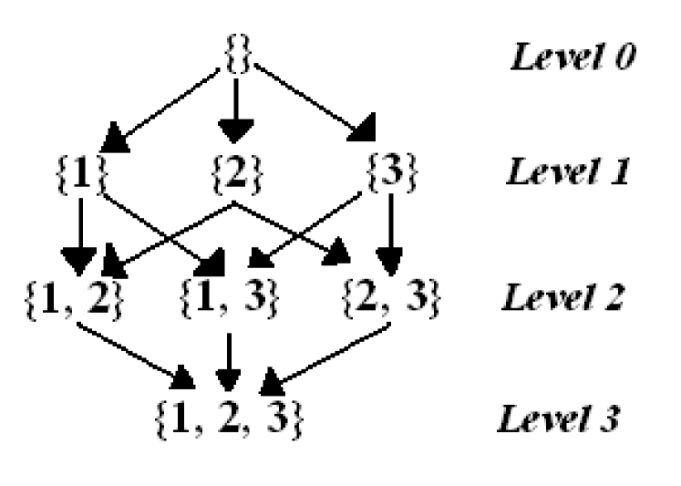
Figure 1: The directed graph of mutational flow between nodes for a three-gene network.

Given some node $\nu=\{i_{1},\dots,i_{n}\}$, define $G_{\nu}\equiv\{\tilde{\nu}\subseteq\{1,\dots,N\}|\nu\subseteq\tilde{\nu}\}$. Therefore, $G_{\nu}$ may be regarded as the subgraph of all nodes which are mutationally accessible from $\nu$. An example of such a subgraph is illustrated in Figure 2.

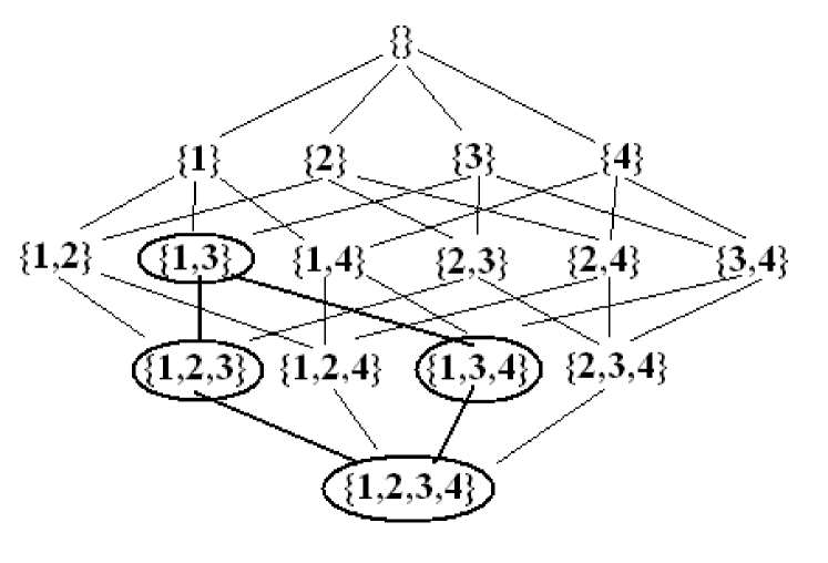
Figure 2: The mutational subgraph $G_{\{1,3\}}$ for a four-gene network.

Let $\Omega$ denote any collection of nodes. Then we may define $G_{\Omega}\equiv\bigcup_{\nu\in\Omega}{G_{\nu}}$. Furthermore, define $\tilde{\Omega}=\{\nu\in\Omega|\Omega\cap G_{\nu}=\nu\}$. Thus, $\tilde{\Omega}$ is the set of all nodes in $\Omega$ such that no node in $\Omega$ is contained within the mutational subgraph of any other node in $\tilde{\Omega}$. Figure 3 gives an example showing the construction of $\tilde{\Omega}$ from $\Omega$.

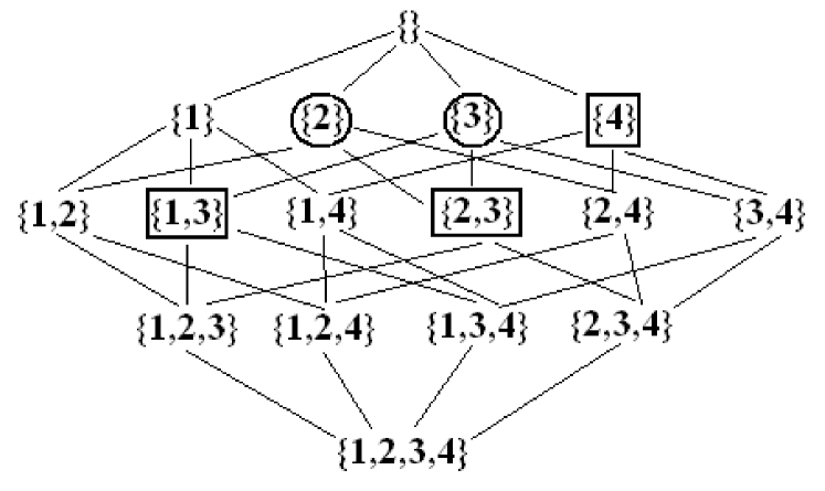
Figure 3: Illustration of $\Omega$ and $\tilde{\Omega}$ in a four-gene network. The nodes circled with rectangles and circles constitute $\Omega$. The nodes circled only with rectangles constitute $\tilde{\Omega}$.

Given some node $\{i_{1},\dots,i_{n}\}$, define $\kappa_{eff}(\{i_{1},\dots,i_{n}\};\mu)=\kappa_{\{i_{1},\dots,i_{n}\}}e^{-(1-\alpha_{i_{1}}-\dots-\alpha_{i_{n}})\mu}$. We then define $\kappa_{max}(\mu)=max\{\kappa_{eff}(\nu;\mu)|\nu\subseteq\{1,\dots,N\}\}$. Finally, given some $\mu$, define $\Omega_{max}(\mu)=\{\nu\subseteq\{1,\dots,N\}|\kappa_{eff}(\nu;\mu)=\kappa_{max}(\mu)\}$.

With these definitions in hand, we are now ready to obtain the structure of the equilibrium solution at a given $\mu$.

III.2 Equilibrium Solution

III.2.1 Determination of $\bar{\kappa}(t=\infty)$

We claim that $\bar{\kappa}(t=\infty)=\kappa_{max}(\mu)$. We prove this in two steps. First of all, we claim that $\bar{\kappa}(t=\infty)=\kappa_{eff}(\nu;\mu)$ for some node $\nu$. Clearly, because $\sum_{\nu\subseteq\{1,\dots,N\}}{\tilde{z}_{\nu}}=1$, it follows that at least one of the $\tilde{z}_{\nu}>0$ at equilibrium. Let $\nu^{\prime}=\{i_{1},\dots,i_{n}\}$ be a node of minimal $n$ such that $\tilde{z}_{\nu^{\prime}}>0$. Then it should be clear that, at equilibrium, we have,

$$0=\frac{d\tilde{z}_{\nu^{\prime}}}{dt}\Bigl{\bracevert}_{t=\infty}=(\kappa_{eff}(\nu^{\prime};\mu)-\bar{\kappa}(t=\infty))\tilde{z}_{\nu^{\prime}}$$ (15)

which, since $\tilde{z}_{\nu^{\prime}}>0$, may be solved to give $\bar{\kappa}(t=\infty)=\kappa_{eff}(\nu^{\prime};\mu)$.

So now suppose that $\bar{\kappa}(t=\infty)\neq\kappa_{max}(\mu)$. Then $\bar{\kappa}(t=\infty)<\kappa_{max}(\mu)$. Such an equilibrium can never be observed because it is unstable. To see this, let $\nu_{max}$ denote a node for which $\kappa_{eff}(\nu_{max};\mu)=\kappa_{max}(\mu)$. Then from Eq. (13) we have, at equilibrium, that,

$$0=\frac{d\tilde{z}_{\nu_{max}}}{dt}\Bigl{\bracevert}_{t=\infty}\geq(\kappa_{eff}(\nu_{max};\mu)-\bar{\kappa}(t=\infty))\tilde{z}_{\nu_{max}}$$ (16)

and so $\tilde{z}_{\nu_{max}}=0$. Clearly, however, any perturbation on $\tilde{z}_{\nu_{max}}$ will push $\tilde{z}_{\nu_{max}}$ away from its equilibrium value. This equilibrium is therefore unstable, and hence, unobservable.

Note that since $\bar{\kappa}(t=\infty)=\kappa_{max}(\mu)$, it follows that the mean equilibrium fitness is a continuous function of $\mu$.

III.2.2 Determining the $\tilde{z}_{\{i_{1},\dots,i_{n}\}}$

To find the equilibrium solution of the reduced system of equations, we first need to determine which $\tilde{z}_{\nu}=0$ at equilibrium. To this end, we begin with the claim that, for $\mu>0$, $\tilde{z}_{\nu}=0$ unless $\nu\in G_{\tilde{\Omega}_{max}(\mu)}$. For suppose there exists $\nu\notin G_{\tilde{\Omega}_{max}(\mu)}$ such that $\tilde{z}_{\nu}\neq 0$ at equilibrium. Then out of the set of all nodes which satisfy the above two properties, we may choose $\nu$ to be of minimal level. We claim that, for any $\tilde{\nu}\subseteq\nu$, we have that $\tilde{\nu}\notin G_{\tilde{\Omega}_{max}(\mu)}$, for otherwise it is clear that $\nu\in G_{\tilde{\nu}}\subseteq G_{\tilde{\Omega}_{max}(\mu)}\Rightarrow\Leftarrow$. Therefore, by the minimality of the level of $\nu$, it follows that $\tilde{z}_{\tilde{\nu}}=0$ whenever $\tilde{\nu}$ is a proper subset of $\nu$. But then the equilibrium equation for $\tilde{z}_{\nu}$ gives $\bar{\kappa}(t=\infty)=\kappa_{eff}(\nu;\mu)$, and so $\kappa_{eff}(\nu;\mu)=\kappa_{max}(\mu)$. Therefore, $\nu\in\Omega_{max}(\mu)$. However, by assumption, $\nu\notin\tilde{\Omega}_{max}(\mu)$, which means that $G_{\nu}$ contains nodes in $\Omega_{max}(\mu)$ which are distinct from $\nu$. Denote one of these nodes by $\tilde{\nu}=\{j_{1},\dots,j_{m}\}$. Then at equilibrium we have, from Eq. (13), that,

$$\frac{d\tilde{z}_{\tilde{\nu}}}{dt}\Bigl{\bracevert}_{t=\infty} = (\kappa_{max}(\mu)-\kappa_{max}(\mu))\tilde{z}_{\tilde{\nu}}+$$ (17)

$$e^{-(1-\alpha_{j_{1}}-\dots-\alpha_{j_{m}})\mu}\sum_{k=0}^{m-1}\sum_{\nu^{\prime}\subset\tilde{\nu}}\times$$

$$\kappa_{\nu^{\prime}}\tilde{z}_{\nu^{\prime}}\prod_{i\in\tilde{\nu}/\nu^{\prime}}{(1-e^{-\alpha_{i}\mu})}$$

$$\geq e^{-(1-\alpha_{j_{1}}-\dots-\alpha_{j_{m}})\mu}\kappa_{\nu}\tilde{z}_{\nu}\prod_{i\in\tilde{\nu}/\nu}{(1-e^{-\alpha_{i}\mu})}$$

$$> 0$$

which is clearly a contradiction. This establishes our claim.

We now argue that our equilibrium solution may be found if we know $\tilde{z}_{\nu}$ for $\nu\in\tilde{\Omega}_{max}(\mu)$. We claim that for any $\nu\in G_{\tilde{\Omega}_{max}(\mu)}$, we may write,

$$\tilde{z}_{\nu}=\sum_{\tilde{\nu}\in\tilde{\Omega}_{max}(\mu)}{\beta_{\tilde{\nu}\nu}(\mu)\tilde{z}_{\tilde{\nu}}}$$ (18)

where the $\beta_{\tilde{\nu}\nu}\geq 0$, and for $\mu>0$ a given $\beta_{\tilde{\nu}\nu}$ is strictly positive if and only if $\nu\in G_{\tilde{\nu}}$. The above expression then holds for all $\nu$, since we simply take $\beta_{\tilde{\nu}\nu}=0$ for $\nu\notin G_{\tilde{\Omega}_{max}(\mu)}$.

We can prove the above formula via induction on the level of the nodes in $G_{\tilde{\Omega}_{max}(\mu)}$. In doing so, we will essentially develop an algorithm for constructing the $\beta_{\tilde{\nu}\nu}$. So, let us start with $n_{min}$, the minimal level nodes $G_{\tilde{\Omega}_{max}(\mu)}$. Then clearly $\nu\in\tilde{\Omega}_{max}(\mu)$, so that $\beta_{\tilde{\nu}\nu}=\delta_{\tilde{\nu}\nu}$, hence the formula is correct for $n_{min}$. So now suppose that, for some $n\geq n_{min}$, the formula is correct for all $m$ such that $n_{min}\leq m\leq n$. Then for a level $n+1$ node in $G_{\tilde{\Omega}_{max}(\mu)}$, denoted by $\{i_{1},\dots,i_{n+1}\}$, we have, at equilibrium, that,

$$0 = (\kappa_{eff}(\{i_{1},\dots,i_{n+1}\};\mu)-\kappa_{max}(\mu))\tilde{z}_{\{i_{1},\dots,i_{n+1}\}}$$ (19)

$$+e^{-(1-\alpha_{i_{1}}-\dots-\alpha_{i_{n+1}})\mu}\sum_{k=0}^{n}\sum_{\{j_{1},\dots,j_{k}\}\subset\{i_{1},\dots,i_{n+1}\}}\times$$

$$\kappa_{\{j_{1},\dots,j_{k}\}}\tilde{z}_{\{j_{1},\dots,j_{k}\}}\prod_{i\in\{i_{1},\dots,i_{n+1}\}/\{j_{1},\dots,j_{k}\}}(1-e^{-\alpha_{i}\mu})$$

$$= (\kappa_{eff}(\{i_{1},\dots,i_{n+1}\};\mu)-\kappa_{max}(\mu))\tilde{z}_{\{i_{1},\dots,i_{n+1}\}}$$

$$+e^{-(1-\alpha_{i_{1}}-\dots-\alpha_{i_{n+1}})\mu}\times$$

$$\sum_{\nu\subset\{i_{1},\dots,i_{n+1}\},\nu\in G_{\tilde{\Omega}_{max}(\mu)}}\kappa_{\nu}\sum_{\tilde{\nu}\in\tilde{\Omega}_{max}(\mu)}\times$$

$$\beta_{\tilde{\nu}\nu}\tilde{z}_{\tilde{\nu}}\prod_{i\in\{i_{1},\dots,i_{n+1}\}/\nu}(1-e^{-\alpha_{i}\mu})$$

$$= (\kappa_{eff}(\{i_{1},\dots,i_{n+1}\};\mu)-\kappa_{max}(\mu))\tilde{z}_{\{i_{1},\dots,i_{n+1}\}}$$

$$+e^{-(1-\alpha_{i_{1}}-\dots-\alpha_{i_{n+1}})\mu}\times$$

$$\sum_{\tilde{\nu}\in\tilde{\Omega}_{max}(\mu)}\tilde{z}_{\tilde{\nu}}\sum_{\nu\subset\{i_{1},\dots,i_{n+1}\},\nu\in G_{\tilde{\nu}}}\times$$

$$\beta_{\tilde{\nu}\nu}\kappa_{\nu}\prod_{i\in\{i_{1},\dots,i_{n+1}\}/\nu}(1-e^{-\alpha_{i}\mu})$$

Now, if $\{i_{1},\dots,i_{n+1}\}\in\tilde{\Omega}_{max}(\mu)$, then $\beta_{\tilde{\nu}\{i_{1},\dots,i_{n+1}\}}=\delta_{\tilde{\nu}\{i_{1},\dots,i_{n+1}\}}$. Otherwise, $\kappa_{eff}(\{i_{1},\dots,i_{n+1};\mu)<\kappa_{max}(\mu)$, so the equilibrium equation may be solved to give,

$$\beta_{\tilde{\nu}\{i_{1},\dots,i_{n+1}\}} = \frac{e^{-(1-\alpha_{i_{1}}-\dots-\alpha_{i_{n+1}})\mu}}{\kappa_{max}(\mu)-\kappa_{eff}(\{i_{1},\dots,i_{n+1}\};\mu)}\times$$

$$\sum_{\nu\subset\{i_{1},\dots,i_{n+1}\},\nu\in G_{\tilde{\nu}}}\beta_{\tilde{\nu}\nu}\kappa_{\nu}\times$$

$$\prod_{i\in\{i_{1},\dots,i_{n+1}\}/\nu}(1-e^{-\alpha_{i}\mu})$$

Note that $\beta_{\tilde{\nu}\{i_{1},\dots,i_{n+1}\}}\geq 0$. Furthermore, if $\{i_{1},\dots,i_{n+1}\}\notin G_{\tilde{\nu}}$, then no proper subset of $\{i_{1},\dots,i_{n+1}\}$ is in $G_{\tilde{\nu}}$. Therefore, $\{\nu\subset\{i_{1},\dots,i_{n+1}\}|\nu\in G_{\tilde{\nu}}\}=\emptyset$, so $\beta_{\tilde{\nu}\{i_{1},\dots,i_{n+1}\}}=0$. Conversely, if $\{i_{1},\dots,i_{n+1}\}\in G_{\tilde{\nu}}$, then since $\{i_{1},\dots,i_{n+1}\}\neq\tilde{\nu}$, it follows that $\{\nu\subset\{i_{1},\dots,i_{n+1}\}|\nu\in G_{\tilde{\nu}}\}\neq\emptyset$. Therefore, the sum in Eq. (20) is nonempty, hence, since the $\beta_{\tilde{\nu}\nu}$ appearing in the sum are all strictly positive, it follows that $\beta_{\tilde{\nu}\{i_{1},\dots,i_{n+1}\}}>0$. This implies that $\beta_{\tilde{\nu}\{i_{1},\dots,i_{n+1}\}}$ is strictly positive if and only if $\{i_{1},\dots,i_{n+1}\}\in G_{\tilde{\nu}}$, which completes the induction step, and proves the claim.

For each $\tilde{\nu}\in\tilde{\Omega}_{max}(\mu)$, we can define $\pi_{\tilde{\nu}}=\sum_{\nu\in G_{\tilde{\nu}}}{\beta_{\tilde{\nu}\nu}}$, and then define $\gamma_{\tilde{\nu}\nu}=\beta_{\tilde{\nu}\nu}/\pi_{\tilde{\nu}}$ and $w_{\tilde{\nu}}=\pi_{\tilde{\nu}\nu}\tilde{z}_{\tilde{\nu}}$. If, for each $\tilde{\nu}$ we also define $\vec{\gamma}_{\tilde{\nu}}=(\gamma_{\tilde{\nu}\nu})$, that is, the vector of all $\gamma_{\tilde{\nu}\nu}$, and if we define $\vec{\tilde{z}}=(\tilde{z}_{\nu})$, then we obtain,

$$\vec{\tilde{z}}=\sum_{\tilde{\nu}\in\tilde{\Omega}_{max}(\mu)}{w_{\tilde{\nu}}\vec{\gamma}_{\tilde{\nu}}}$$ (21)

where $\sum_{\tilde{\nu}\in\tilde{\Omega}_{max}(\mu)}{w_{\tilde{\nu}}}=1$.

Note that the $\vec{\gamma}_{\tilde{\nu}}$ form a linearly independent set of vectors. Therefore, if $\tilde{\Omega}_{max}(\mu)$ contains more than one node, then the equilibrium solution of the reduced system of equations is not unique, but rather is defined by the parallelipiped $\{\sum_{\tilde{\nu}\in\tilde{\Omega}_{max}(\mu)}{w_{\tilde{\nu}}\vec{\gamma}_{\tilde{\nu}}}|\sum_{\tilde{\nu}\in\tilde{\Omega}_{max}(\mu)}{w_{\tilde{\nu}}}=1,w_{\tilde{\nu}}\geq 0\}$.

As mentioned earlier, the degeneracy in the equilibrium behavior follows from the neglect of backmutations in the limit of infinite sequence length. The various nodes in $\tilde{\Omega}_{max}(\mu)$ become mutationally decoupled in this limit, which can cause the largest eigenvalue of the mutation matrix ${\bf B}$ to be degenerate. However, for finite sequence lengths, the quasispecies dynamics will always converge to a unique solution. In particular, if we start with the initial condition $z_{\emptyset}=1$, then for finite sequence lengths we will converge to the unique equilibrium solution. Because all nodes are mutationally connected in the infinite sequence length limit with this initial condition, we make the assumption that the way to find the infinite sequence length equilibrium which is the limit of the finite sequence length equilibria is to find the infinite sequence length equilibrium starting from the initial condition $z_{\emptyset}=1$. This allows us to break the eigenstate degeneracy in a canonical manner.

In the appendices, we describe a fixed-point iteration approach for finding the equilibrium solution of the model. Within this algorithm, we also use the initial condition $z_{\emptyset}=1$ as the analogous approach to the one above for finding the infinite sequence length equilibrium which is the limit of the finite sequence length equilibria.

Finally, the treatment thus far has been finding the equilibrium solution of the reduced system of equations for $\mu>0$. The equilibrium solution for $\mu=0$ is obtained by taking the limit of the $\mu>0$ solutions, so that $\vec{\tilde{z}}(\mu=0)=\lim_{\mu\rightarrow 0^{+}}{\vec{\tilde{z}}(\mu)}$.

III.2.3 Construction of the phase diagram

From the previous development it is clear that the nodes in $\tilde{\Omega}_{max}(\mu)$ may be regarded as “source” nodes which dictate the solution. To understand how the solution changes with $\mu$, we therefore need to determine how $\tilde{\Omega}_{max}(\mu)$ depends on $\mu$.

We claim the following: That there exist a finite number of $\mu$, which we denote by $\mu_{1},\dots,\mu_{N}$, where $0\leq\mu_{1}<\dots<\mu_{N}<\infty$, for which $\{(\kappa_{\{i_{1},\dots,i_{n}\}},\alpha_{i_{1}}+\dots+\alpha_{i_{n}})|\{i_{1},\dots,i_{n}\}\in\Omega_{max}(\mu)\}$ contains distinct elements. In any interval $(\mu_{i-1},\mu_{i})$, $\Omega_{max}(\mu)$ is constant, and may therefore be denoted by $\Omega_{i}$. The $\Omega_{i}$ are all disjoint, and $\Omega_{i}\cup\Omega_{i+1}\subseteq\Omega_{max}(\mu_{i})$.

We begin proving this claim by introducing one more definition. Let $\Sigma_{\neq}$ denote the set of all sets of nodes, such that a collection of nodes $\Omega$ is a member of $\Sigma_{\neq}$ if and only if $\{(\kappa_{\{i_{1},\dots,i_{n}\}},\alpha_{i_{1}}+\dots+\alpha_{i_{n}})|\{i_{1},\dots,i_{n}\}\in\Omega\}$ contains distinct elements.

Note that since there are $2^{N}$ nodes, there are $2^{2^{N}}$ sets of nodes, hence $\Sigma_{\neq}$ consists of a finite number of elements. Given some $\Omega_{\neq}\in\Sigma_{\neq}$, we claim that $\Omega_{max}(\mu)=\Omega_{\neq}$ for at most one $\mu$. To show this, suppose that there exist $\mu_{1}<\mu_{2}$ for which $\Omega_{max}(\mu_{1})=\Omega_{max}(\mu_{2})=\Omega_{\neq}$. Choose any two nodes $\{i_{1},\dots,i_{n}\}$, $\{j_{1},\dots,j_{m}\}$ in $\Omega_{\neq}$, and note that $\kappa_{\{i_{1},\dots,i_{n}\}}e^{-(1-\alpha_{i_{1}}-\dots-\alpha_{i_{n}})\mu_{1}}=\kappa_{\{j_{1},\dots,j_{m}\}}e^{-(1-\alpha_{j_{1}}-\dots-\alpha_{j_{m}})\mu_{1}}=\kappa_{max}(\mu_{1})$, and similarly for $\mu_{2}$. However, $a_{1}e^{-b_{1}x}=a_{2}e^{-b_{2}x}$ and $a_{1}e^{-b_{1}y}=a_{2}e^{-b_{2}y}$ implies that $e^{-b_{1}(y-x)}=e^{-b_{2}(y-x)}$, so that $b_{1}=b_{2}$ and hence $a_{1}=a_{2}$. Therefore, $\kappa_{\{i_{1},\dots,i_{n}\}}=\kappa_{\{j_{1},\dots,j_{m}\}}$ and $\alpha_{i_{1}}+\dots+\alpha_{i_{n}}=\alpha_{j_{1}}+\dots+\alpha_{j_{m}}$, so $\{(\kappa_{\{i_{1},\dots,i_{n}\}},\alpha_{i_{1}}+\dots+\alpha_{i_{n}})|\{i_{1},\dots,i_{n}\}\in\Omega_{\neq}\}$ does not contain distinct elements. Because this contradicts our assumption about $\Omega_{\neq}$, it follows that $\Omega_{max}(\mu)=\Omega_{\neq}$ for at most one $\mu$.

So, since $\Sigma_{\neq}$ contains a finite number of elements, it follows that there are a finite number of $\mu$ for which $\Omega_{max}(\mu)$ satisfies the property that $\{(\kappa_{\{i_{1},\dots,i_{n}\}},\alpha_{i_{1}}+\dots+\alpha_{i_{n}})|\{i_{1},\dots,i_{n}\}\in\Omega_{max}(\mu)\}$ contains distinct elements. We can denote these $\mu$ by $\mu_{1},\dots,\mu_{N}$, where we assume that $0\leq\mu_{1}<\dots<\mu_{N}<\infty$.

Note that if a collection of nodes $\Omega$ has the property that $\tilde{\Omega}\neq\Omega$, then $\Omega$ must be a collection in $\Sigma_{\neq}$. This is easy to see: $\Omega$ contains some $\{i_{1},\dots,i_{n}\}$ for which there exists a distinct $\{j_{1},\dots,j_{m}\}\in\Omega$ where $\{j_{1},\dots,j_{m}\}\in G_{\{i_{1},\dots,i_{n}\}}$. Therefore $\alpha_{i_{1}}+\dots+\alpha_{i_{n}}<\alpha_{j_{1}}+\dots+\alpha_{j_{m}}$, which proves our contention.

We now prove that $\Omega_{max}(\mu)$ is some constant, which we denote by $\Omega_{i}$, over $(\mu_{i-1},\mu_{i})$. Given some $\mu_{0}\in(\mu_{i-1},\mu_{i})$, let $\mu_{+}=\sup\{\tilde{\mu}\in(\mu_{0},\mu_{i})|\Omega_{max}(\mu)=\Omega_{max}(\mu_{0})\mbox{ }\forall\mbox{ }\mu\in(\mu_{0},\tilde{\mu})\}$ ($\sup$ stands for “supremum”, which is the least upper bound of a set of real numbers. If ${\bf S}$ is a set of real numbers with an upper bound, then $A\equiv\sup{\bf S}$ exists, and satisfies the following properties: (1) $A$ is an upper bound for ${\bf S}$. (2) If $B$ is any upper bound of ${\bf S}$, then $A\leq B$. (2) If $B<A$, then there exists at least one element of ${\bf S}$ which exceeds $B$.). Clearly, $\mu_{+}\leq\mu_{i}$. We claim that $\mu_{+}=\mu_{i}$. To show this, note first of all that $\Omega_{max}(\mu)=\Omega_{max}(\mu_{0})$ for all $\mu\in(\mu_{0},\mu_{+})$, and that for any $\tilde{\mu}>\mu_{+}$, there exists $\mu\in[\mu_{+},\tilde{\mu})$ such that $\Omega_{max}(\mu)\neq\Omega_{max}(\mu_{0})$. For given any $\mu^{\prime}\in(\mu_{0},\mu_{+})$, we have, by definition of $\sup$, that there exists some $\tilde{\mu}\in(\mu^{\prime},\mu_{+})$ such that $\Omega_{max}(\mu)=\Omega_{max}(\mu_{0})$ for all $\mu\in(\mu_{0},\tilde{\mu})$. In particular, this implies that $\Omega_{max}(\mu^{\prime})=\Omega_{max}(\mu_{0})$. Furthermore, if there exists $\tilde{\mu}>\mu_{+}$ for which $\Omega_{max}(\mu)=\Omega_{max}(\mu_{0})$ for all $\mu\in[\mu_{+},\tilde{\mu})$, then $\Omega_{max}(\mu)=\Omega_{max}(\mu_{0})$ for all $\mu\in(\mu_{0},\tilde{\mu})$, contradicting the definition of $\mu_{+}$.

Now, suppose $\Omega_{max}(\mu_{+})\notin\Sigma_{\neq}$. Then we can write $\kappa_{\{i_{1},\dots,i_{n}\}}=\kappa_{+}$ and $\alpha_{i_{1}}+\dots+\alpha_{i_{n}}=\alpha_{+}$ for all $\{i_{1},\dots,i_{n}\}\in\Omega_{max}(\mu_{+})$. Then since $\kappa_{max}(\mu_{+})=\kappa_{+}e^{-(1-\alpha_{+})\mu_{+}}$, it follows by continuity that $\kappa_{+}e^{-(1-\alpha_{+})\mu}>\kappa_{eff}(\nu;\mu)$ for $\nu\notin\Omega_{max}(\mu_{+})$ in some neighborhood $(\mu_{+}-\delta,\mu_{+}+\delta)$. But this implies that $\Omega_{max}(\mu)=\Omega_{max}(\mu_{+})$ over $(\mu_{+}-\delta,\mu_{+}+\delta)$. Since $\Omega_{max}(\mu_{0})=\Omega_{max}(\mu)$ over $(\mu_{+}-\delta,\mu_{+})$, we obtain that $\Omega_{max}(\mu)=\Omega_{max}(\mu_{0})$ over $(\mu_{0},\mu_{+}+\delta)$, contradicting the definition of $\mu_{+}$.

We have just shown that $\Omega_{max}(\mu_{+})\in\Sigma_{\neq}$. Since $\Omega_{max}(\mu)\notin\Sigma_{\neq}$ over $(\mu_{i-1},\mu_{i})$, we must have that $\mu_{+}=\mu_{i}$. Using a similar argument with $\inf$, we can show that $\Omega_{max}(\mu)=\Omega_{max}(\mu_{0})$ over $(\mu_{i-1},\mu_{0})$, and so $\Omega_{max}(\mu)$ is constant on $(\mu_{i-1},\mu_{i})$ ($\inf$ stands for “infimum”, and is defined as the greatest lower bound of a set of real numbers. It satisfies properties analogous to those of $\sup$).

Suppose for two $i,j$ with $i<j$, we have $\Omega_{i}$ and $\Omega_{j}$ are not disjoint. Then they share at least one node, and so, by the nature of the two sets, we must have that $\Omega_{i}=\Omega_{j}$. Define $\kappa$ to be $\kappa_{\{i_{1},\dots,i_{n}\}}$ for any node in $\Omega_{i}$, $\Omega_{j}$, and $\alpha$ to be $\alpha_{i_{1}}+\dots+\alpha_{i_{n}}$. Now, $\Omega_{max}(\mu_{i})$ contains some node $\{i_{1},\dots,i_{n}\}\notin\Omega_{i}$ such that $\kappa_{eff}(\{i_{1},\dots,i_{n}\};\mu)<\kappa e^{-(1-\alpha)\mu}$ for $\mu$ in $(\mu_{i-1},\mu_{i})\cup(\mu_{j-1},\mu_{j})$. But if for $x_{1}<x_{2}$ we have that $a_{1}e^{-b_{1}x_{1}}<a_{2}e^{-b_{2}x_{1}}$ and $a_{1}e^{-b_{1}x_{2}}<a_{2}e^{-b_{2}x_{2}}$, then $(a_{1}/a_{2})e^{-(b_{1}-b_{2})x_{1}}<1$ and $(a_{1}/a_{2})e^{-(b_{1}-b_{2})x_{2}}<1$. Since $(a_{1}/a_{2})e^{-(b_{1}-b_{2})x}$ is monotone decreasing or increasing, it follows that $(a_{1}/a_{2})e^{-(b_{1}-b_{2})x}<1$ on $(x_{1},x_{2})$, or equivalently, $a_{1}e^{-b_{1}x}<a_{2}e^{-b_{2}x}$. Therefore, $\kappa_{max}(\mu_{i})=\kappa_{eff}(\{i_{1},\dots,i_{n}\};\mu_{i})<\kappa e^{-(1-\alpha)\mu_{i}}\Rightarrow\Leftarrow$. The $\Omega_{i}$ are thus all disjoint, as claimed.

Finally, since $\kappa_{max}(\mu)$ is continuous, we have that $\lim_{\mu\rightarrow\mu_{i}^{-}}{\kappa_{max}(\mu)}=\kappa_{max}(\mu_{i})$. If $\nu\in\Omega_{i}$, then this gives $\kappa_{max}(\mu_{i})=\kappa_{eff}(\nu;\mu_{i})$. Similarly, considering $\lim_{\mu\rightarrow\mu_{i}^{+}}{\kappa_{max}(\mu)}$ gives that $\kappa_{max}(\mu_{i})=\kappa_{eff}(\nu;\mu_{i})$ for $\nu\in\Omega_{i+1}$. Therefore, $\Omega_{i},\Omega_{i+1}\subseteq\Omega_{max}(\mu_{i})$, so $\Omega_{i}\cup\Omega_{i+1}\subseteq\Omega_{max}(\mu_{i})$, as claimed.

The various $\Omega_{i}$ may therefore be regarded as defining different “phases” in the equilibrium behavior of the model. Physically, each “phase” is defined by a set of “source nodes,” which dictate which genes in the genome are knocked out, and which are not. The transition from $\Omega_{i}$ to $\Omega_{i+1}$ corresponds to certain genes in the genome becoming knocked out, and perhaps other genes becoming viable again. This transition can happen more than once, and so we refer to the series of $\Omega_{i}\rightarrow\Omega_{i+1}$ transitions as an “error cascade.”

Because $\kappa_{eff}(\{1,\dots,N\};\mu)=1$, for sufficiently large $\mu$, $\kappa_{eff}(\{1,\dots,N\};\mu)>\kappa_{eff}(\nu;\mu)$ for any $\nu\neq\{1,\dots,N\}$. Therefore, for sufficiently large $\mu$, $\Omega_{max}(\mu)=\{\{1,\dots,N\}\}$. Since $\Omega_{max}(\mu)$ is constant on $(\mu_{N},\infty)$, it follows that $\Omega_{max}(\mu)=\{\{1,\dots,N\}\}$ on $(\mu_{N},\infty)$. Thus, the final transition from $\Omega_{N}$ to $\Omega_{N+1}$ corresponds to delocalization over the entire genome space, which is simply the error catastrophe.

III.2.4 Finding the $z_{l_{1},\dots,l_{N}}$

Once we have determined $\bar{\kappa}(t=\infty)$, we can in principle obtain the population fractions $z_{l_{1},\dots,l_{N}}$ in the various Hamming classes. The problem is that, if $z_{\emptyset}=0$, then for any finite values of $l_{1},\dots,l_{n}$, we get that $z_{l_{1},\dots,l_{N}}=0$. To show this, suppose we can find $l_{1},\dots,l_{N}$ such that $z_{l_{1},\dots,l_{N}}>0$ at equilibrium. Of the $l_{1},\dots,l_{N}$ for which $z_{l_{1},\dots,l_{N}}>0$, choose a set of indices $l_{1}^{\prime},\dots,l_{N}^{\prime}$ such that $l_{1}^{\prime}+\dots+l_{N}^{\prime}$ is as small as possible. Note that if $z_{l_{1},\dots,l_{N}}=z_{l_{1}^{\prime}-l_{1}^{\prime\prime},\dots,l_{N}^{\prime}-l_{N}^{\prime\prime}}$, with $(l_{1}^{\prime\prime},\dots,l_{N}^{\prime\prime})\neq(0,\dots,0)$, then $z_{l_{1},\dots,l_{N}}=0$.

Now, let the nonzero $l_{i}^{\prime}$ be denoted by $l_{i_{1}}^{\prime},\dots,l_{i_{n}}^{\prime}$. Then $\kappa_{l_{1}^{\prime},\dots,l_{N}^{\prime}}=\kappa_{\{i_{1},\dots,i_{n}\}}$, and we have, from Eq. (11), that, at equilibrium,

$$0=\frac{dz_{l_{1}^{\prime},\dots,l_{N}^{\prime}}}{dt}\Bigl{\bracevert}_{t=\infty}=(\kappa_{\{i_{1},\dots,i_{n}\}}e^{-\mu}-\bar{\kappa}(t=\infty))z_{l_{1}^{\prime},\dots,l_{N}^{\prime}}$$ (22)

which gives $\bar{\kappa}(t=\infty)=\kappa_{\{i_{1},\dots,i_{n}\}}e^{-\mu}$. But, $\bar{\kappa}(t=\infty)\geq\kappa_{\{i_{1},\dots,i_{n}\}}e^{-(1-\alpha_{i_{1}}-\dots-\alpha_{i_{n}})\mu}$. Therefore, $e^{-\mu}\geq e^{-(1-\alpha_{i_{1}}-\dots-\alpha_{i_{n}})\mu}$, and so $\alpha_{i_{1}}+\dots+\alpha_{i_{n}}=0$, hence $n=0$. But then $z_{l_{1}^{\prime},\dots,l_{N}^{\prime}}=z_{\emptyset}>0\Rightarrow\Leftarrow$. This proves our claim.

If $\tilde{\Omega}_{max}(\mu)=\emptyset$, then the above claim does not present us with any problem. We can simply recursively solve Eq. (11) at equilibrium for all the $z_{l_{1},\dots,l_{N}}$. But once any delocalization occurs, it is impossible to solve for the equilibrium distribution in terms of the Hamming classes. However, we can recursively obtain the distribution of another class of population fractions, as follows: Given some collection of indices $\{i_{1},\dots,i_{n}\}$, another collection of indices $\{j_{1},\dots,j_{k}\}\subseteq\{i_{1},\dots,i_{n}\}$, and a collection of Hamming distances $l_{1},\dots,l_{N}$, we define $\tilde{z}_{\{j_{1},\dots,j_{k}\}}(\vec{l}_{\{i_{1},\dots,i_{n}\}})$ and $z_{\{j_{1},\dots,j_{k}\}}(\vec{l}_{\{i_{1},\dots,i_{n}\}})$ as,

$$\tilde{z}_{\{j_{1},\dots,i_{k}\}}(\vec{l}_{\{i_{1},\dots,i_{n}\}})=\sum_{l_{j_{1}}=1}^{\infty}\cdot\dots\cdot\sum_{l_{j_{k}}=1}^{\infty}{z_{l_{j_{1}}{\bf e}_{j_{1}}+\dots+l_{j_{k}}{\bf e}_{j_{k}}+\sum_{i\in\{1,\dots,N\}/\{i_{1},\dots,i_{n}\}}l_{i}{\bf e}_{i}}}$$

$$z_{\{j_{1},\dots,j_{k}\}}(\vec{l}_{\{i_{1},\dots,i_{n}\}})=\sum_{l_{j_{1}}=0}^{\infty}\cdot\dots\cdot\sum_{l_{j_{k}}=0}^{\infty}{z_{l_{j_{1}}{\bf e}_{j_{1}}+\dots+l_{j_{k}}{\bf e}_{j_{k}}+\sum_{i\in\{1,\dots,N\}/\{i_{1},\dots,i_{n}\}}l_{i}{\bf e}_{i}}}$$ (23)

It is possible to show that,

$$z_{\{j_{1},\dots,j_{k}\}}(\vec{l}_{\{i_{1},\dots,i_{n}\}}) = \sum_{l=0}^{k}\sum_{\{j_{1}^{\prime},\dots,j_{l}^{\prime}\}\subseteq\{j_{1},\dots,j_{k}\}}\tilde{z}_{\{j_{1}^{\prime},\dots,j_{l}^{\prime}\}}(\vec{l}_{\{i_{1},\dots,i_{n}\}})$$ (24)

and hence that,

$$\tilde{z}_{\{j_{1},\dots,j_{k}\}}(\vec{l}_{\{i_{1},\dots,i_{n}\}}) = \sum_{l=0}^{k}(-1)^{k-l}\sum_{\{j_{1}^{\prime},\dots,j_{l}^{\prime}\}\subseteq\{j_{1},\dots,j_{k}\}}z_{\{j_{1}^{\prime},\dots,j_{l}^{\prime}\}}(\vec{l}_{\{i_{1},\dots,i_{n}\}})$$ (25)

We may then derive the expression for $d\tilde{z}_{\{i_{1},\dots,i_{n}\}}(\vec{l}_{\{i_{1},\dots,i_{n}\}})/dt$. Since the derivation uses techniques similar to those used in Appendices A and B, we simply state the final result, which is,

$$\frac{d\tilde{z}_{\{i_{1},\dots,i_{n}\}}(\vec{l}_{\{i_{1},\dots,i_{n}\}})}{dt} = e^{-(1-\alpha_{i_{1}}-\dots-\alpha_{i_{n}})\mu}\sum_{k=0}^{n}\sum_{\{j_{1},\dots,j_{k}\}\subseteq\{i_{1},\dots,i_{n}\}}\sum_{\stackrel{{\scriptstyle l_{i}^{\prime}=0}}{{i\in\{1,\dots,N\}/\{i_{1},\dots,i_{n}\}}}}^{l_{i}}\prod_{i\in\{1,\dots,N\}/\{i_{1},\dots,i_{n}\}}{\frac{(\alpha_{i}\mu)^{l_{i}^{\prime}}}{l_{i}^{\prime}!}}\times$$ (26)

$$\Pi_{j\in\{i_{1},\dots,i_{n}\}/\{j_{1},\dots,j_{k}\}}(1-e^{-\alpha_{j}\mu})\times$$

$$\kappa_{\{j_{1},\dots,j_{k}\}}(\vec{l}_{\{i_{1},\dots,i_{n}\}}-\vec{l}^{\prime}_{\{i_{1},\dots,i_{n}\}})\tilde{z}_{\{j_{1},\dots,j_{k}\}}(\vec{l}_{\{i_{1},\dots,i_{n}\}}-\vec{l}^{\prime}_{\{i_{1},\dots,i_{n}\}})$$

$$-\bar{\kappa}(t)\tilde{z}_{\{i_{1},\dots,i_{n}\}}(\vec{l}_{\{i_{1},\dots,i_{n}\}})$$

where $\kappa_{\{j_{1},\dots,j_{k}\}}(\vec{l}_{\{i_{1},\dots,i_{n}\}})=\kappa_{\{j_{1},\dots,j_{k}\}\cup\{j_{1}^{\prime},\dots,j_{l}^{\prime}\}}$, where $\{j_{1}^{\prime},\dots,j_{l}^{\prime}\}$ are the indices of the nonzero Hamming distances in $\vec{l}_{\{i_{1},\dots,i_{n}\}}$.

We claim that, at equilibrium, $\tilde{z}_{\nu}(\vec{l}_{\nu})>0$ only if $\nu\in G_{\tilde{\nu}}$ for some $\tilde{\nu}\in\tilde{\Omega}_{max}(\mu)$ for which $\tilde{z}_{\tilde{\nu}}>0$. For if $\tilde{z}_{\nu}(\vec{l}_{\nu})>0$, let $\tilde{\nu}=\{i_{1},\dots,i_{n}\}\subseteq\nu$ be a node of minimal level for which there exists $\vec{l}_{\tilde{\nu}}$ such that $\tilde{z}_{\tilde{\nu}}(\vec{l}_{\tilde{\nu}})>0$. Note then that for any proper subset $\{j_{1},\dots,j_{k}\}\subset\{i_{1},\dots,i_{n}\}$, we must have that $\tilde{z}_{\{j_{1},\dots,j_{k}\}}(\vec{l}_{\{i_{1},\dots,i_{n}\}})=0$. This implies that, at equilibrium,

$$0 = \frac{d\tilde{z}_{\{i_{1},\dots,i_{n}\}}(\vec{l}_{\{i_{1},\dots,i_{n}\}})}{dt}$$ (27)

$$= e^{-(1-\alpha_{i_{1}}-\dots-\alpha_{i_{n}})\mu}\times$$

$$\sum_{\stackrel{{\scriptstyle l_{i}^{\prime}=0}}{{i\in\{1,\dots,N\}/\{i_{1},\dots,i_{n}\}}}}^{l_{i}}\prod_{i\in\{1,\dots,N\}/\{i_{1},\dots,i_{n}\}}{\frac{(\alpha_{i}\mu)^{l_{i}^{\prime}}}{l_{i}^{\prime}!}}\times$$

$$\kappa_{\{i_{1},\dots,i_{n}\}}(\vec{l}_{\{i_{1},\dots,i_{n}\}}-\vec{l}^{\prime}_{\{i_{1},\dots,i_{n}\}})\times$$

$$\tilde{z}_{\{i_{1},\dots,i_{n}\}}(\vec{l}_{\{i_{1},\dots,i_{n}\}}-\vec{l}^{\prime}_{\{i_{1},\dots,i_{n}\}})$$

$$-\bar{\kappa}(t=\infty)\tilde{z}_{\{i_{1},\dots,i_{n}\}}(\vec{l}_{\{i_{1},\dots,i_{n}\}})$$

Among all $\vec{l}_{\{i_{1},\dots,i_{n}\}}$ for which $\tilde{z}_{\{i_{1},\dots,i_{n}\}}(\vec{l}_{\{i_{1},\dots,i_{n}\}})>0$, there exists an $\vec{l}^{\prime\prime}_{\{i_{1},\dots,i_{n}\}}$ such that $\sum_{i\in\{1,\dots,N\}/\{i_{1},\dots,i_{n}\}}{l_{i}^{\prime\prime}}$ is minimal. Then we obtain,

$$0 = \frac{d\tilde{z}_{\{i_{1},\dots,i_{n}\}}(\vec{l}^{\prime\prime}_{\{i_{1},\dots,i_{n}\}})}{dt}\Bigl{\bracevert}_{t=\infty}$$ (28)

$$= (\kappa_{\{i_{1},\dots,i_{n}\}}(\vec{l}^{\prime\prime}_{\{i_{1},\dots,i_{n}\}})e^{-(1-\alpha_{i_{1}}-\dots-\alpha_{i_{n}})\mu}-\bar{\kappa}(t))\times$$

$$\tilde{z}_{\{i_{1},\dots,i_{n}\}}(\vec{l}^{\prime\prime}_{\{i_{1},\dots,i_{n}\}})$$

which gives $\bar{\kappa}(t=\infty)=\kappa_{\{i_{1},\dots,i_{n}\}}(\vec{l}^{\prime\prime}_{\{i_{1},\dots,i_{n}\}})e^{-(1-\alpha_{i_{1}}-\dots-\alpha_{i_{n}})\mu}$. Now, let $i_{1}^{\prime},\dots,i_{m}^{\prime}$ denote the indices of the nonzero Hamming distances in $\vec{l}_{\{i_{1},\dots,i_{n}\}}$. Then $\kappa_{\{i_{1},\dots,i_{n}\}}=\kappa_{\{i_{1},\dots,i_{n}\}\cup\{i_{1}^{\prime},\dots,i_{m}^{\prime}\}}$. But since $\bar{\kappa}(t=\infty)\geq\kappa_{\{i_{1},\dots,i_{n}\}\cup\{i_{1}^{\prime},\dots,i_{m}^{\prime}\}}e^{-(1-\alpha_{i_{1}}-\dots-\alpha_{i_{n}}-\alpha_{i_{1}^{\prime}}-\dots-\alpha_{i_{m}^{\prime}})\mu}$, we get $\alpha_{i_{1}^{\prime}}+\dots+\alpha_{i_{m}^{\prime}}=0$, so $m=0$. Therefore $\bar{\kappa}(t=\infty)=\kappa_{eff}(\tilde{\nu};\mu)$, so since $\tilde{z}_{\tilde{\nu}}>0$, we have $\tilde{\nu}\in\tilde{\Omega}_{max}(\mu)$.

The $\tilde{z}_{\nu}(\vec{l}_{\nu})$ may be obtained recursively from Eq. (27), starting with the values of $\tilde{z}_{\nu}$ for $\nu\in\tilde{\Omega}_{max}(\mu)$. The idea is that, starting with the values of $\tilde{z}_{\nu}$ for $\nu\in\tilde{\Omega}_{max}(\mu)$, we may compute $\tilde{z}_{\nu}(\vec{l}_{\nu})$ recursively. We then proceed down the levels, computing the $\tilde{z}_{\nu}(\vec{l}_{\nu})$ using the values of $\tilde{z}_{\nu}(\vec{l}_{\nu}-\vec{l}^{\prime}_{\nu})$ and $\tilde{z}_{\tilde{\nu}}(\vec{l}_{\tilde{\nu}})$ for $\tilde{\nu}\subset\nu$. Note then that instead of computing the $z_{l_{1},\dots,l_{N}}$, which will be $0$ as soon as any delocalization occurs, we first sum over a set of gene indices containing the delocalized genes as a subset, and only compute the population distribution for finite Hamming distances of the localized genes.

III.3 Localization Lengths

In this subsection, we compute various localization lengths associated with the population distribution. Specifically, given a node $\{i_{1},\dots,i_{n}\}$, and some $i\notin\{i_{1},\dots,i_{n}\}$, we define two localization lengths, $\langle l_{i}\rangle_{\{i_{1},\dots,i_{n}\}}$ and $\tilde{\langle l_{i}\rangle}_{\{i_{1},\dots,i_{n}\}}$, as follows:

$$\langle l_{i}\rangle_{\{i_{1},\dots,i_{n}\}}\equiv\sum_{l_{i_{1}}=0}^{\infty}\cdot\dots\cdot\sum_{l_{i_{n}}=0}^{\infty}\sum_{l_{i}=1}^{\infty}{l_{i}z_{l_{i_{1}}{\bf e}_{i_{1}}+\dots+l_{i_{n}}{\bf e}_{i_{n}}+l_{i}{\bf e}_{i}}}$$

(29)

$$\tilde{\langle l_{i}\rangle}_{\{i_{1},\dots,i_{n}\}}\equiv\sum_{l_{i_{1}}=1}^{\infty}\cdot\dots\cdot\sum_{l_{i_{n}}=1}^{\infty}\sum_{l_{i}=1}^{\infty}{l_{i}z_{l_{i_{1}}{\bf e}_{i_{1}}+\dots+l_{i_{n}}{\bf e}_{i_{n}}+l_{i}{\bf e}_{i}}}$$

Note that,

$$\langle l_{i}\rangle_{\{i_{1},\dots,i_{n}\}}=\sum_{k=0}^{n}\sum_{\{j_{1},\dots,j_{k}\}\subseteq\{i_{1},\dots,i_{n}\}}{\tilde{\langle l_{i}\rangle}_{\{j_{1},\dots,j_{k}\}}}$$ (31)

and so, in analogy with $z_{\{i_{1},\dots,i_{n}\}}$ and $\tilde{z}_{\{i_{1},\dots,i_{n}\}}$, we have that,

$$\tilde{\langle l_{i}\rangle}_{\{i_{1},\dots,i_{n}\}}=\sum_{k=0}^{n}(-1)^{n-k}\sum_{\{j_{1},\dots,j_{k}\}\subseteq\{i_{1},\dots,i_{n}\}}{\langle l_{i}\rangle_{\{j_{1},\dots,j_{k}\}}}$$ (32)

We also define the localization length $\langle l_{i}\rangle$ by,

$$\langle l_{i}\rangle=\sum_{l_{1}=0}^{\infty}\cdot\dots\cdot\sum_{l_{N}=0}^{\infty}{l_{i}z_{l_{1},\dots,l_{N}}}$$ (33)

Note that $\langle l_{i}\rangle=\langle l_{i}\rangle_{\{1,\dots,N\}/\{i\}}=\sum_{n=0}^{N-1}\sum_{\{i_{1},\dots,i_{n}\}\subseteq\{1,\dots,N\}/\{i\}}\tilde{\langle l_{i}\rangle}_{\{i_{1},\dots,i_{n}\}}$, and so is finite if and only if all the $\tilde{\langle l_{i}\rangle}_{\{i_{1},\dots,i_{n}\}}$ are finite.

We can compute $\tilde{\langle l_{i}\rangle}_{\{i_{1},\dots,i_{n}\}}$ at equilibrium by finding the time derivative and setting it to $0$. In Appendix B we show that,

$$\frac{d\tilde{\langle l_{i}\rangle}_{\{i_{1},\dots,i_{n}\}}}{dt} = (\kappa_{eff}(\{i_{1},\dots,i_{n},i\};\mu)-\bar{\kappa}(t))\tilde{\langle l_{i}\rangle}_{\{i_{1},\dots,i_{n}\}}$$ (34)

$$+\alpha_{i}\mu e^{-(1-\alpha_{i_{1}}-\dots-\alpha_{i_{n}}-\alpha_{i})\mu}(\kappa_{\{i_{1},\dots,i_{n}\}}\tilde{z}_{\{i_{1},\dots,i_{n}\}}+\kappa_{\{i_{1},\dots,i_{n},i\}}\tilde{z}_{\{i_{1},\dots,i_{n},i\}})$$

$$+e^{-(1-\alpha_{i_{1}}-\dots-\alpha_{i_{n}}-\alpha_{i})\mu}\sum_{k=0}^{n-1}\sum_{\{j_{1},\dots,j_{k}\}\subset\{i_{1},\dots,i_{n}\}}\times$$

$$(\kappa_{\{j_{1},\dots,j_{k},i\}}\tilde{\langle l_{i}\rangle}_{\{j_{1},\dots,j_{k}\}}+\alpha_{i}\mu\kappa_{\{j_{1},\dots,j_{k}\}}\tilde{z}_{\{j_{1},\dots,j_{k}\}}+\alpha_{i}\mu\kappa_{\{j_{1},\dots,j_{k},i\}}\tilde{z}_{\{j_{1},\dots,j_{k},i\}})\times$$

$$\prod_{j\in\{i_{1},\dots,i_{n}\}/\{j_{1},\dots,j_{k}\}}(1-e^{-\alpha_{j}\mu})$$

Therefore, at equilibrium, we get,

$$\tilde{\langle l_{i}\rangle}_{\{i_{1},\dots,i_{n}\}} = \alpha_{i}\mu\frac{e^{-(1-\alpha_{i_{1}}-\dots-\alpha_{i_{n}}-\alpha_{i})\mu}}{\bar{\kappa}(t=\infty)-\kappa_{eff}(\{i_{1},\dots,i_{n},i\};\mu)}(\kappa_{\{i_{1},\dots,i_{n}\}}\tilde{z}_{\{i_{1},\dots,i_{n}\}}+\kappa_{\{i_{1},\dots,i_{n},i\}}\tilde{z}_{\{i_{1},\dots,i_{n},i\}})$$ (35)

$$+\frac{e^{-(1-\alpha_{i_{1}}-\dots-\alpha_{i_{n}}-\alpha_{i})\mu}}{\bar{\kappa}(t=\infty)-\kappa_{eff}(\{i_{1},\dots,i_{n},i\};\mu)}\sum_{k=0}^{n-1}\sum_{\{j_{1},\dots,j_{k}\}\subset\{i_{1},\dots,i_{n}\}}\times$$

$$(\kappa_{\{j_{1},\dots,j_{k},i\}}\tilde{\langle l_{i}\rangle}_{\{j_{1},\dots,j_{k}\}}+\alpha_{i}\mu\kappa_{\{j_{1},\dots,j_{k}\}}\tilde{z}_{\{j_{1},\dots,j_{k}\}}+\alpha_{i}\mu\kappa_{\{j_{1},\dots,j_{k},i\}}\tilde{z}_{\{j_{1},\dots,j_{k},i\}})\times$$

$$\prod_{j\in\{i_{1},\dots,i_{n}\}/\{j_{1},\dots,j_{k}\}}(1-e^{-\alpha_{j}\mu})$$

We can characterize the behavior of the $\tilde{\langle l_{i}\rangle}_{\{i_{1},\dots,i_{n}\}}$. First of all, we claim that $\tilde{\langle l_{i}\rangle}_{\{i_{1},\dots,i_{n}\}}=0$ if and only if $\tilde{z}_{\{i_{1},\dots,i_{n},i\}}=0$. Secondly, we claim that $\tilde{\langle l_{i}\rangle}_{\{i_{1},\dots,i_{n}\}}=\infty$ if and only if $\{j_{1},\dots,j_{k},i\}\in\tilde{\Omega}_{max}(\mu)$ with $\tilde{z}_{\{j_{1},\dots,j_{k},i\}}>0$ for some $\{j_{1},\dots,j_{k}\}\subseteq\{i_{1},\dots,i_{n}\}$.

To show this, note first of all that, from physical considerations, $\tilde{\langle l_{i}\rangle}_{\{i_{1},\dots,i_{n}\}}=0$ if $\tilde{z}_{\{i_{1},\dots,i_{n},i\}}=0$. If $\tilde{z}_{\{i_{1},\dots,i_{n},i\}}>0$, then $\{i_{1},\dots,i_{n},i\}\in G_{\tilde{\Omega}_{max}(\mu)}$, and so, since $\bar{\kappa}(t=\infty)\geq\kappa_{eff}(\{i_{1},\dots,i_{n}\};\mu)$, it follows that $\tilde{\langle l_{i}\rangle}_{\{i_{1},\dots,i_{n}\}}>0$. This establishes the first part of our claim.

So now suppose that $\{j_{1},\dots,j_{k},i\}\in\tilde{\Omega}_{max}(\mu)$, with $\tilde{z}_{\{j_{1},\dots,j_{k},i\}}>0$ for some $\{j_{1},\dots,j_{k}\}\subseteq\{i_{1},\dots,i_{n}\}$. Then $\bar{\kappa}(t=\infty)=\kappa_{eff}(\{j_{1},\dots,j_{k},i\};\mu)$, and so,

$$\tilde{\langle l_{i}\rangle}_{\{j_{1},\dots,j_{k}\}} = \alpha_{i}\mu\frac{e^{-(1-\alpha_{j_{1}}-\dots-\alpha_{j_{k}}-\alpha_{i})\mu}}{\bar{\kappa}(t=\infty)-\kappa_{eff}(\{j_{1},\dots,j_{k},i\};\mu)}\times$$ (36)

$$\kappa_{\{j_{1},\dots,j_{k},i\}}\tilde{z}_{\{j_{1},\dots,j_{k},i\}}=\infty$$

which of course implies that $\tilde{\langle l_{i}\rangle}_{\{i_{1},\dots,i_{n}\}}=\infty$.

To prove the converse, let us suppose that $\tilde{\langle l_{i}\rangle}_{\{i_{1},\dots,i_{n}\}}=\infty$. Let us choose $\{j_{1},\dots,j_{k}\}\subseteq\{i_{1},\dots,i_{n}\}$ to be the minimal level subset for which $\tilde{\langle l_{i}\rangle}_{\{j_{1},\dots,j_{k}\}}=\infty$. Then if $\bar{\kappa}(t=\infty)>\kappa_{eff}(\{j_{1},\dots,j_{k},i\};\mu)$, it is clear from the expression for $d\tilde{\langle l_{i}\rangle}_{\{j_{1},\dots,j_{k}\}}/dt$ that $\tilde{\langle l_{i}\rangle}_{\{j_{1}^{\prime},\dots,j_{l}^{\prime}\}}=\infty$ for some $\{j_{1}^{\prime},\dots,j_{l}^{\prime}\}\subset\{j_{1},\dots,j_{k}\}$, with $0\leq l\leq k-1$. But this contradicts the minimality of $k$, hence $\bar{\kappa}(t=\infty)=\kappa_{eff}(\{j_{1},\dots,j_{k},i\};\mu)$, so since $\tilde{z}_{\{j_{1},\dots,j_{k},i\}}>0$, it follows that $\{j_{1},\dots,j_{k},i\}\in\tilde{\Omega}_{max}(\mu)$. This proves the converse, which establishes the second part of our claim.

III.4 A Simple Example

We now illustrate the theory developed above using a simple two-gene “network” as an example. We assume a genome containing two identical genes, so that $\alpha_{1}=\alpha_{2}=1/2$, and we choose the following growth parameters: $\kappa_{\emptyset}=10$, $\kappa_{\{1\}}=\kappa_{\{2\}}=5$, and $\kappa_{\{1,2\}}=1$.

With these parameters, the system exhibits two localization to delocalization transitions. First, for $\mu\in[0,2\ln 2)$ we have $\tilde{\Omega}_{max}(\mu)=\emptyset$. For $\mu\in(2\ln 2,2\ln 5)$ we have $\tilde{\Omega}_{max}(\mu)=\{\{1\},\{2\}\}$. The error catastrophe occurs at $\mu=2\ln 5$.

We determined the equilibrium behavior of the model by solving the finite sequence length equations for $L=40$ and $S=2$. The details may be found in Appendix C. Figure 4 shows a plot of $\bar{\kappa}(t=\infty)$ from the simulation results and from our theory. Figure 5 shows plots of $\tilde{z}_{\emptyset}$, $\tilde{z}_{\{1\}}$, $\tilde{z}_{\{2\}}$, and $\tilde{z}_{\{1,2\}}$ from the simulation results and from theory.

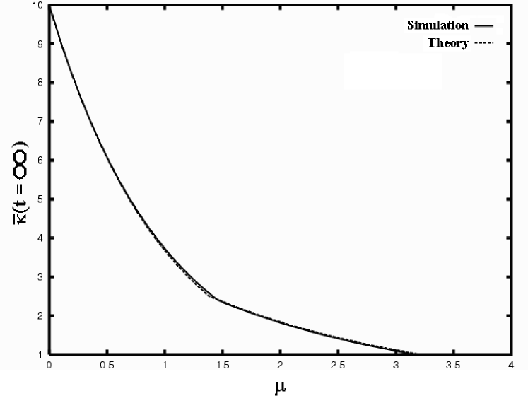
Figure 4: Plot of $\bar{\kappa}(t=\infty)$ from both simulation and theory.

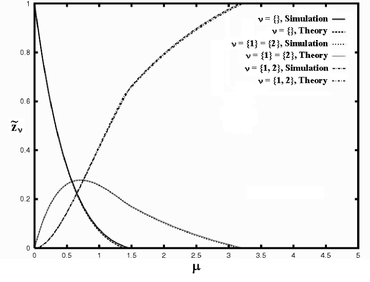
Figure 5: Plots of $\tilde{z}_{\emptyset}$, $\tilde{z}_{\{1\}}$, $\tilde{z}_{\{2\}}$, and $\tilde{z}_{\{1,2\}}$ from both simulation and theory. By symmetry, $w_{\{1\}}=w_{\{2\}}=1/2$ when $\tilde{\Omega}_{max}(\mu)=\{\{1\},\{2\}\}$.

IV Discussion

The first point to note about the solution of the quasispecies equations for a gene network is that, unlike the single gene model, which exhibits a single “error catastrophe,” the multiple gene model exhibits a series of localization to delocalization transitions which we term an “error cascade.” The reason for this is that as the mutation rate is increased, the selective advantage for maintaining functional copies of certain genes in the genome is no longer sufficiently strong to localize the population distribution about the corresponding master sequences, and delocalization occurs in the corresponding sequence spaces.

The more a given gene or set of genes contributes to the fitness of an organism, the larger $\mu$ will have to be to induce delocalization in the corresponding sequence spaces. Eventually, by making $\mu$ sufficiently large, the selective advantage for maintaining any functional genes in the genome will disappear, and the result is complete delocalization over all sequence spaces, corresponding to the error catastrophe.

The prediction of an error cascade suggests an approach for determining the selective advantage of maintaining certain genes in a genome. Currently, the standard method for determining whether a gene is “essential” is by knocking it out, and then seeing if the organism survives. By knocking out each of the genes, one can construct a “deletion set” for a given organism, consisting of the minimal set of genes necessary for the organism to survive Winzeler et al. (1999).

While knowledge of the deletion set of an organism is important, it does not explain why the organism should maintain functional copies of other, “nonessential” genes. One possibility is that these “nonessential” do confer a fitness advantage to the organism, however, the time scale on which organisms are observed to grow during knockout experiments is simply too short to resolve these fitness differences.

Thus, an alternative approach to the deletion set method is to have organisms grow at various mutagen concentrations. By determining which genes get knocked out at the corresponding mutation rates, it is possible to determine the relative importance of various genes to the fitness of an organism. Such an experiment is likely to be difficult to perform. Nevertheless, if successful, it would provide a considerably more powerful approach than the deletion set method for determining fitness advantages of various genes.

The results in this paper also shed light on a phenomenon which C.O. Wilke termed the “survival of the flattest” Wilke and Adami (2003). Briefly, what Wilke (and others) showed was that at low mutation rates, a population will localize in a region of sequence space which has high fitness. At higher mutation rates, a population will relocalize in a region of sequence space which may not have maximal fitness, but is mutationally robust Wilke and Adami (2003).

The error cascade is exactly a relocalization from a region of high fitness but low mutational support to a region of lower fitness but higher mutational support. The reason for this is that the fitness landscape becomes progressively flatter as more and more genes are knocked out, because the more genes are knocked out, the smaller the fraction of the genome which is involved in determining the fitness of the organism.

This implies that an error cascade is necessary for the “survival of the flattest” principle to hold. Robustness in this sense is therefore conferred by modularity in the genome. That is, robustness does not arise because an individual gene may remain functional after several point-mutations, but rather arises from the fact that the organism can remain viable even if entire regions (e.g. “genes”) of the genome are knocked out (it should be noted that the idea that mutational robustness is conferred by modularity in the genome has been discussed before Wilke and Adami (2003)).

To see this point more clearly, one can consider a “robust” landscape in which the genome consists of a single gene. However, unlike the single-fitness peak landscape, the organism is viable out to some Hamming class $l_{via}$. Therefore, if $D_{H}(\sigma,\sigma_{0})=l$, then $\kappa_{\sigma}=1$ if $l>l_{via}$, otherwise $\kappa_{\sigma}=\kappa_{l}$, where $\kappa_{0}\geq\kappa_{1}\geq\dots\geq\kappa_{l_{via}}>1$. Using techniques similar to the ones used in this paper (neglect of backmutations and stability criterion for equilibria), it is possible to show that the equilibrium mean fitness is exactly $\kappa_{0}e^{-\mu}$, unchanged from the single-fitness peak results. Thus, in contrast to robustness studies which consider finite sequence lengths and do not have a well-defined viability cutoff Krakauer and Plotkin (2002), in the limit of infinite sequence length there is no selective advantage in having a genome which can sustain a finite number of point mutations and remain viable.

V Conclusions

This paper developed an extension of the quasispecies model for arbitrary gene networks. We considered the case of conservative replication and a genome-independent replication error probability. We showed that, instead of a single error catastrophe, the model exhibits a series of localization to delocalization transitions, termed an “error cascade.”

While the numerical example we used in this paper was relatively simple (in order to clearly illustrate the theory developed), it is possible to have nontrivial delocalization behavior, depending on the choice of the landscape. For example, it is possible that certain genes which are knocked out in one phase can become reactivated again in the following phase. That is, instead of a delocalization, one can have a re-localization to source nodes not contained in the mutational subgraphs of the source nodes in the previous phase. This implies that the $\tilde{z}_{\nu}$ can exhibit discontinuous behavior. The types of equilibrium behaviors possible is something which will be explored in future research.

Future research also will involve incorporating more details to the multiple-gene model introduced in this paper. For example, one extension is to move away from the “single-fitness peak” assumption for each gene. Another natural extension is to study the equilibrium behavior of the multiple-gene quasispecies equations for the case of semiconservative replication. While this is a subject for future work, we hypothesize that many of the semiconservative results would be essentially unchanged from the conservative ones. Thus, we claim that at equilibrium, we would still have that $\bar{\kappa}(t=\infty)=\kappa_{max}(\mu)$, only this time $\kappa_{eff}(\nu;\mu)$ is computed by replacing $e^{-\mu}$ with $2e^{-\mu/2}-1$. We also claim that we would still have that $\tilde{\Omega}_{max}(\mu)$ define the “source” nodes of the equilibrium solution. Indeed, we hypothesize that, for semiconservative replication, Eq. (13) becomes,

$$\frac{d\tilde{z}_{\{i_{1},\dots,i_{n}\}}}{dt} = (\kappa_{eff}(\{i_{1},\dots,i_{n}\};\mu)-\bar{\kappa}(t))\tilde{z}_{\{i_{1},\dots,i_{n}\}}$$ (37)

$$+\sum_{k=0}^{n-1}\sum_{\{j_{1},\dots,j_{k}\}\subset\{i_{1},\dots,i_{n}\}}\kappa_{\{j_{1},\dots,j_{k}\}}\tilde{z}_{\{j_{1},\dots,j_{k}\}}\times$$

$$\prod_{i\in\{i_{1},\dots,i_{n}\}/\{j_{1},\dots,j_{k}\}}(1-e^{-\alpha_{i}\mu/2})$$

Finally, another subject for future work is the incorporation of repair into our network model. In Tannenbaum and Shakhnovich (2003); Tannenbaum et al. (2003) it was assumed that only one gene controlled repair. By assuming that several genes control repair, then, in analogy with fitness, we hypothesize that instead of a single “repair catastrophe” Tannenbaum and Shakhnovich (2003); Tannenbaum et al. (2003), we obtain a series of localization to delocalization transitions over the repair gene sequence spaces, a “repair cascade.”

Appendix A Derivation of the Reduced System of Equations

In this appendix, we derive Eq. (13) from Eq. (11). To this end, define,

$$z_{\{i_{1},\dots,i_{n}\}}=\sum_{l_{i_{1}}=0}^{\infty}\cdot\dots\cdot\sum_{l_{i_{n}}=0}^{\infty}{z_{l_{i_{1}}{\bf e}_{i_{1}}+\dots+l_{i_{n}}{\bf e}_{i_{n}}}}$$ (38)

We then have that,

$$\frac{dz_{\{i_{1},\dots,i_{n}\}}}{dt} = \sum_{l_{i_{1}}=0}^{\infty}\cdot\dots\cdot\sum_{l_{i_{n}}=0}^{\infty}(e^{-\mu}\sum_{l_{i_{1}}^{\prime}=0}^{l_{i_{1}}}\cdot\dots\cdot\sum_{l_{i_{n}}^{\prime}=0}^{l_{i_{n}}}\times$$ (39)

$$\frac{\kappa_{(l_{i_{1}}-l_{i_{1}}^{\prime}){\bf e}_{i_{1}}+\dots+(l_{i_{n}}-l_{i_{n}}^{\prime}){\bf e}_{i_{n}}}}{l_{i_{1}}^{\prime}!\cdot\dots\cdot l_{i_{n}}^{\prime}!}(\alpha_{i_{1}}\mu)^{l_{i_{1}}^{\prime}}\cdot\dots\cdot(\alpha_{i_{n}}\mu)^{l_{i_{n}}^{\prime}}z_{(l_{i_{1}}-l_{i_{1}}^{\prime}){\bf e}_{i_{1}}+\dots+(l_{i_{n}}-l_{i_{n}}^{\prime}){\bf e}_{i_{n}}}$$

$$-\bar{\kappa}(t)z_{l_{i_{1}}{\bf e}_{i_{1}}+\dots+l_{i_{n}}{\bf e}_{i_{n}}})$$

$$= e^{-\mu}\sum_{l_{i_{1}}^{\prime}=0}^{\infty}\cdot\dots\cdot\sum_{l_{i_{n}}^{\prime}=0}^{\infty}{\frac{1}{l_{i_{1}}^{\prime}!\cdot\dots\cdot l_{i_{n}}^{\prime}!}(\alpha_{i_{1}}\mu)^{l_{i_{1}}^{\prime}}\cdot\dots\cdot(\alpha_{i_{n}}\mu)^{l_{i_{n}}^{\prime}}}\times$$

$$\sum_{l_{i_{1}}=l_{i_{1}}^{\prime}}^{\infty}\cdot\dots\cdot\sum_{l_{i_{n}}=l_{i_{n}}^{\prime}}^{\infty}{\kappa_{(l_{i_{1}}-l_{i_{1}}^{\prime}){\bf e}_{i_{1}}+\dots+(l_{i_{n}}-l_{i_{n}}^{\prime}){\bf e}_{i_{n}}}z_{(l_{i_{1}}-l_{i_{1}}^{\prime}){\bf e}_{i_{1}}+\dots+(l_{i_{n}}-l_{i_{n}}^{\prime}){\bf e}_{i_{n}}}}-\bar{\kappa}(t)z_{\{i_{1},\dots,i_{n}\}}$$

$$= e^{-(1-\alpha_{i_{1}}-\dots-\alpha_{i_{n}})\mu}\sum_{k_{i_{1}}=0}^{\infty}\cdot\dots\cdot\sum_{k_{i_{n}}=0}^{\infty}{\kappa_{k_{i_{1}}{\bf e}_{i_{1}}+\dots+k_{i_{n}}{\bf e}_{i_{n}}}z_{k_{i_{1}}{\bf e}_{i_{1}}+\dots+k_{i_{n}}{\bf e}_{i_{n}}}}-\bar{\kappa}(t)z_{\{i_{1},\dots,i_{n}\}}$$

$$= e^{-(1-\alpha_{i_{1}}-\dots-\alpha_{i_{n}})\mu}\sum_{k=0}^{n}\sum_{\{j_{1},\dots,j_{k}\}\subseteq\{i_{1},\dots,i_{n}\}}{\kappa_{\{j_{1},\dots,j_{k}\}}\tilde{z}_{\{j_{1},\dots,j_{k}\}}}-\bar{\kappa}(t)z_{\{i_{1},\dots,i_{n}\}}$$

We now claim that,

$$\tilde{z}_{\{i_{1},\dots,i_{n}\}}=\sum_{k=0}^{n}(-1)^{n-k}\sum_{\{j_{1},\dots,j_{k}\}\subseteq\{i_{1},\dots,i_{n}\}}{z_{\{j_{1},\dots,j_{k}\}}}$$ (40)

This can be proved by induction. For $n=0$ this statement is clearly true, since $z_{\emptyset}=\tilde{z}_{\emptyset}$. Suppose then, that for some $n\geq 0$, the statement is true for all $0\leq m\leq n$. Then we have,

$$z_{\{i_{1},\dots,i_{n+1}\}} = \sum_{k=0}^{n+1}\sum_{\{j_{1},\dots,j_{k}\}\subseteq\{i_{1},\dots,i_{n+1}\}}{\tilde{z}_{\{j_{1},\dots,j_{k}\}}}$$

$$= \tilde{z}_{\{i_{1},\dots,i_{n+1}\}}$$

$$+\sum_{k=0}^{n}\sum_{\{j_{1},\dots,j_{k}\}\subseteq\{i_{1},\dots,i_{n+1}\}}{\tilde{z}_{\{j_{1},\dots,j_{k}\}}}$$

and so,

$$\tilde{z}_{\{i_{1},\dots,i_{n+1}\}} = z_{\{i_{1},\dots,i_{n+1}\}}$$ (42)

$$-\sum_{k=0}^{n}\sum_{\{j_{1},\dots,j_{k}\}\subseteq\{i_{1},\dots,i_{n+1}\}}\sum_{l=0}^{k}(-1)^{k-l}\times$$

$$\sum_{\{j_{1}^{\prime},\dots,j_{l}^{\prime}\}\subseteq\{j_{1},\dots,j_{k}\}}{z_{\{j_{1}^{\prime},\dots,j_{k}^{\prime}\}}}$$

Now, for each set $\{j_{1},\dots,j_{k}\}$ appearing in the sum, a given subset $\{j_{1}^{\prime},\dots,j_{l}^{\prime}\}$ occurs only once. The $k$-element sets $\{j_{1},\dots,j_{k}\}$ which contain $\{j_{1}^{\prime},\dots,j_{l}^{\prime}\}$ as a subset must be of the form $\{j_{1}^{\prime},\dots,j_{l}^{\prime}\}\cup\{j_{1}^{\prime\prime},\dots,j_{k-l}^{\prime\prime}\}$, where $\{j_{1}^{\prime\prime},\dots,j_{k-l}^{\prime\prime}\}\subseteq\{i_{1},\dots,i_{n+1}\}/\{j_{1}^{\prime},\dots,j_{l}^{\prime}\}$. Therefore, there are ${n+1-l}\choose{k-l}$ distinct $k$-element sets which contain $\{j_{1},^{\prime},\dots,j_{l}^{\prime}\}$. Rearranging the sum, we obtain,

$$\tilde{z}_{\{i_{1},\dots,i_{n+1}\}} = z_{\{i_{1},\dots,i_{n+1}\}}$$ (43)

$$-\sum_{l=0}^{n}\sum_{\{j_{1},\dots,j_{l}\}\subseteq\{i_{1},\dots,i_{n+1}\}}z_{\{j_{1},\dots,j_{l}\}}\times$$

$$\sum_{k=l}^{n}(-1)^{k-l}{{n+1-l}\choose{k-l}}$$

$$= z_{\{i_{1},\dots,i_{n+1}\}}$$

$$-\sum_{l=0}^{n}\sum_{\{j_{1},\dots,j_{l}\}\subseteq\{i_{1},\dots,i_{n+1}\}}z_{\{j_{1},\dots,j_{l}\}}(-(-1)^{n+1-l})$$

$$= \sum_{l=0}^{n+1}(-1)^{n+1-l}\sum_{\{j_{1},\dots,j_{l}\}\subseteq\{i_{1},\dots,i_{n+1}\}}z_{\{j_{1},\dots,j_{l}\}}$$

This completes the induction step, and proves the claim.

We are almost ready to derive the expression for $d\tilde{z}_{\{i_{1},\dots,i_{n}\}}/dt$. Before doing so, we state the following identity, which we will need in our calculation:

$$\prod_{i=1}^{n}(1-\alpha_{i})=\sum_{k=0}^{n}(-1)^{k}\sum_{\{i_{1},\dots,i_{k}\}\subseteq\{1,\dots,n\}}\alpha_{i_{1}}\cdot\dots\cdot\alpha_{i_{k}}$$ (44)

We now have,

$$\frac{d\tilde{z}_{\{i_{1},\dots,i_{n}\}}}{dt} = \sum_{k=0}^{n}(-1)^{n-k}\sum_{\{j_{1},\dots,j_{k}\}\subseteq\{i_{1},\dots,i_{n}\}}\frac{dz_{\{j_{1},\dots,j_{k}\}}}{dt}$$ (45)

$$= \sum_{k=0}^{n}(-1)^{n-k}\sum_{\{j_{1},\dots,j_{k}\}\subseteq\{i_{1},\dots,i_{n}\}}(e^{-(1-\alpha_{j_{1}}-\dots-\alpha_{j_{k}})\mu}\sum_{l=0}^{k}\sum_{\{j_{1}^{\prime},\dots,j_{l}^{\prime}\}\subseteq\{j_{1},\dots,j_{k}\}}{\kappa_{\{j_{1}^{\prime},\dots,j_{l}^{\prime}\}}\tilde{z}_{\{j_{1}^{\prime},\dots,j_{l}^{\prime}\}}}$$

$$-\bar{\kappa}(t)z_{\{j_{1},\dots,j_{k}\}})$$

$$= \sum_{l=0}^{n}\sum_{\{j_{1},\dots,j_{l}\}\subseteq\{i_{1},\dots,i_{n}\}}\kappa_{\{j_{1},\dots,j_{l}\}}\tilde{z}_{\{j_{1},\dots,j_{l}\}}\times$$

$$\sum_{k=l}^{n}(-1)^{n-k}\sum_{\{j_{1}^{\prime},\dots,j_{k-l}^{\prime}\}\subseteq\{i_{1},\dots,i_{n}\}/\{j_{1},\dots,j_{l}\}}e^{-(1-\alpha_{j_{1}}-\dots-\alpha_{j_{l}}-\alpha_{j_{1}}^{\prime}-\dots-\alpha_{j_{k-l}^{\prime}})\mu}$$

$$-\bar{\kappa}(t)\tilde{z}_{\{i_{1},\dots,i_{n}\}}$$

$$= \sum_{l=0}^{n}\sum_{\{j_{1},\dots,j_{l}\}\subseteq\{i_{1},\dots,i_{n}\}}\kappa_{\{j_{1},\dots,j_{l}\}}\tilde{z}_{\{j_{1},\dots,j_{l}\}}\times$$

$$e^{-(1-\alpha_{j_{1}}-\dots-\alpha_{j_{l}})\mu}\sum_{k-l=0}^{n-l}(-1)^{n-l}(-1)^{k-l}\sum_{\{j_{1}^{\prime},\dots,j_{k-l}^{\prime}\}\subseteq\{i_{1},\dots,i_{n}\}/\{j_{1},\dots,j_{l}\}}e^{\alpha_{j_{1}^{\prime}}\mu}\cdot\dots\cdot e^{\alpha_{j_{k-l}^{\prime}}\mu}$$

$$-\bar{\kappa}(t)\tilde{z}_{\{i_{1},\dots,i_{n}\}}$$

$$= \sum_{l=0}^{n}\sum_{\{j_{1},\dots,j_{l}\}\subseteq\{i_{1},\dots,i_{n}\}}\kappa_{\{j_{1},\dots,j_{l}\}}\tilde{z}_{\{j_{1},\dots,j_{l}\}}\times$$

$$(-1)^{n-l}e^{-(1-\alpha_{j_{1}}-\dots-\alpha_{j_{l}})\mu}\prod_{i\in\{i_{1},\dots,i_{n}\}/\{j_{1},\dots,j_{l}\}}(1-e^{\alpha_{i}\mu})$$

$$-\bar{\kappa}(t)\tilde{z}_{\{i_{1},\dots,i_{n}\}}$$

$$= e^{-(1-\alpha_{i_{1}}-\dots-\alpha_{i_{n}})\mu}\sum_{l=0}^{n}\sum_{\{j_{1},\dots,j_{l}\}\subseteq\{i_{1},\dots,i_{n}\}}\kappa_{\{j_{1},\dots,j_{l}\}}\tilde{z}_{\{j_{1},\dots,j_{l}\}}\prod_{i\in\{i_{1},\dots,i_{n}\}/\{j_{1},\dots,j_{l}\}}(1-e^{-\alpha_{i}\mu})$$

$$-\bar{\kappa}(t)\tilde{z}_{\{i_{1},\dots,i_{n}\}}$$

which is exactly Eq. (13).

Appendix B Derivation of the Localization Lengths

In this section we derive the expression for $d\tilde{\langle l_{i}\rangle}_{\{i_{1},\dots,i_{n}\}}/dt$. We have,

$$\frac{d\langle l_{i}\rangle_{\{i_{1},\dots,i_{n}\}}}{dt} = \sum_{l_{i_{1}}=0}^{\infty}\cdot\dots\cdot\sum_{l_{i_{n}}=0}^{\infty}\sum_{l_{i}=0}^{\infty}l_{i}(e^{-\mu}\sum_{l_{i_{1}}^{\prime}=0}^{l_{i_{1}}}\cdot\dots\cdot\sum_{l_{i_{n}}^{\prime}=0}^{l_{i_{n}}}\sum_{l_{i}^{\prime}=0}^{l_{i}}\frac{\kappa_{(l_{i_{1}}-l_{i_{1}}^{\prime}){\bf e}_{i_{1}}+\dots+(l_{i_{n}}-l_{i_{n}}^{\prime}){\bf e}_{i_{n}}+(l_{i}-l_{i}^{\prime}){\bf e}_{i}}}{l_{i_{1}}^{\prime}!\cdot\dots\cdot l_{i_{n}}^{\prime}!l_{i}^{\prime}!}\times$$ (46)

$$(\alpha_{i_{1}}\mu)^{l_{i_{1}}^{\prime}}\cdot\dots\cdot(\alpha_{i_{n}}\mu)^{l_{i_{n}}^{\prime}}(\alpha_{i}\mu)^{l_{i}^{\prime}}z_{(l_{i_{1}}-l_{i_{1}}^{\prime}){\bf e}_{i_{1}}+\dots+(l_{i_{n}}-l_{i_{n}}^{\prime}){\bf e}_{i_{n}}+(l_{i}-l_{i}^{\prime}){\bf e}_{i}}$$

$$-\bar{\kappa}(t)z_{l_{i_{1}}{\bf e}_{i_{1}}+\dots+l_{i_{n}}{\bf e}_{i_{n}}+l_{i}{\bf e}_{i}})$$

$$= e^{-\mu}\sum_{l_{i_{1}}^{\prime}=0}^{\infty}\cdot\dots\cdot\sum_{l_{i_{n}}^{\prime}=0}^{\infty}\sum_{l_{i}^{\prime}=0}^{\infty}\frac{(\alpha_{i_{1}}\mu)^{l_{i_{1}}^{\prime}}\cdot\dots\cdot(\alpha_{i_{n}}\mu)^{l_{i_{n}}^{\prime}}(\alpha_{i}\mu)^{l_{i}^{\prime}}}{l_{i_{1}}^{\prime}!\cdot\dots\cdot l_{i_{n}}^{\prime}!l_{i}^{\prime}!}\times$$

$$\sum_{k_{i_{1}}=0}^{\infty}\cdot\dots\cdot\sum_{k_{i_{n}}=0}^{\infty}\sum_{k_{i}=0}^{\infty}(k_{i}+l_{i}^{\prime})\kappa_{k_{i_{1}}{\bf e}_{i_{1}}+\dots+k_{i_{n}}{\bf e}_{i_{n}}+k_{i}{\bf e}_{i}}z_{k_{i_{1}}{\bf e}_{i_{1}}+\dots+k_{i_{n}}{\bf e}_{i_{n}}+k_{i}{\bf e}_{i}}$$

$$-\bar{\kappa}(t)\langle l_{i}\rangle_{\{i_{1},\dots,i_{n}\}}$$

$$= e^{-(1-\alpha_{i_{1}}-\dots-\alpha_{i_{n}}-\alpha_{i})\mu}(\sum_{k=0}^{n}\sum_{\{j_{1},\dots,j_{k}\}\subseteq\{i_{1},\dots,i_{n}\}}{\kappa_{\{j_{1},\dots,j_{k},i\}}\tilde{\langle l_{i}\rangle}_{\{j_{1},\dots,j_{k}\}}}$$

$$+\alpha_{i}\mu\sum_{k=0}^{n+1}\sum_{\{j_{1},\dots,j_{k}\}\subseteq\{i_{1},\dots,i_{n},i\}}{\kappa_{\{j_{1},\dots,j_{k}\}}\tilde{z}_{\{j_{1},\dots,j_{k}\}}})-\bar{\kappa}(t)\langle l_{i}\rangle_{\{i_{1},\dots,i_{n}\}}$$

$$= e^{-(1-\alpha_{i_{1}}-\dots-\alpha_{i_{n}}-\alpha_{i})\mu}\sum_{k=0}^{n}\sum_{\{j_{1},\dots,j_{k}\}\subseteq\{i_{1},\dots,i_{n}\}}\times$$

$$(\kappa_{\{j_{1},\dots,j_{k},i\}}\tilde{\langle l_{i}\rangle}_{\{j_{1},\dots,j_{k}\}}+\alpha_{i}\mu\kappa_{\{j_{1},\dots,j_{k}\}}\tilde{z}_{\{j_{1},\dots,j_{k}\}}+\alpha_{i}\mu\kappa_{\{j_{1},\dots,j_{k},i\}}\tilde{z}_{\{j_{1},\dots,j_{k},i\}})$$

$$-\bar{\kappa}(t)\langle l_{i}\rangle_{\{i_{1},\dots,i_{n}\}}$$

We therefore have that,

$$\frac{d\tilde{\langle l_{i}\rangle}_{\{i_{1},\dots,i_{n}\}}}{dt} = \sum_{k=0}^{n}(-1)^{n-k}\sum_{\{j_{1},\dots,j_{k}\}\subseteq\{i_{1},\dots,i_{n}\}}{\frac{d\langle l_{i}\rangle_{\{j_{1},\dots,j_{k}\}}}{dt}}$$ (47)

$$= \sum_{k=0}^{n}(-1)^{n-k}\sum_{\{j_{1},\dots,j_{k}\}\subseteq\{i_{1},\dots,i_{n}\}}[e^{-(1-\alpha_{j_{1}}-\dots-\alpha_{j_{k}}-\alpha_{i})\mu}\sum_{l=0}^{k}\sum_{\{j_{1}^{\prime},\dots,j_{l}^{\prime}\}\subseteq\{j_{1},\dots,j_{k}\}}\times$$

$$(\kappa_{\{j_{1}^{\prime},\dots,j_{l}^{\prime},i\}}\tilde{\langle l_{i}\rangle}_{\{j_{1}^{\prime},\dots,j_{l}^{\prime}\}}+\alpha_{i}\mu\kappa_{\{j_{1}^{\prime},\dots,j_{l}^{\prime}\}}\tilde{z}_{\{j_{1}^{\prime},\dots,j_{l}^{\prime}\}}+\alpha_{i}\mu\kappa_{\{j_{1}^{\prime},\dots,j_{l}^{\prime},i\}}\tilde{z}_{\{j_{1}^{\prime},\dots,j_{l}^{\prime},i\}})$$

$$-\bar{\kappa}(t)\langle l_{i}\rangle_{\{j_{1},\dots,j_{k}\}}]$$

$$= \sum_{l=0}^{n}\sum_{\{j_{1}^{\prime},\dots,j_{l}^{\prime}\}\subseteq\{i_{1},\dots,i_{n}\}}(-1)^{n-l}e^{-(1-\alpha_{j_{1}^{\prime}}-\dots-\alpha_{j_{l}}^{\prime}-\alpha_{i})\mu}\times$$

$$(\kappa_{\{j_{1}^{\prime},\dots,j_{l}^{\prime},i\}}\tilde{\langle l_{i}\rangle}_{\{j_{1}^{\prime},\dots,j_{l}^{\prime}\}}+\alpha_{i}\mu\kappa_{\{j_{1}^{\prime},\dots,j_{l}^{\prime}\}}\tilde{z}_{\{j_{1}^{\prime},\dots,j_{l}^{\prime}\}}+\alpha_{i}\mu\kappa_{\{j_{1}^{\prime},\dots,j_{l}^{\prime},i\}}\tilde{z}_{\{j_{1}^{\prime},\dots,j_{l}^{\prime},i\}})\times$$

$$\sum_{k-l=0}^{n-l}(-1)^{k-l}\sum_{\{j_{1},\dots,j_{k-l}\}\subseteq\{i_{1},\dots,i_{n}\}/\{j_{1}^{\prime},\dots,j_{l}^{\prime}\}}e^{\alpha_{j_{1}}\mu}\cdot\dots\cdot e^{\alpha_{j_{k-l}}\mu}$$

$$-\bar{\kappa}(t)\tilde{\langle l_{i}\rangle}_{\{i_{1},\dots,i_{n}\}}$$

$$= e^{-(1-\alpha_{i_{1}}-\dots-\alpha_{i_{n}}-\alpha_{i})\mu}\sum_{k=0}^{n}\sum_{\{j_{1},\dots,j_{k}\}\subseteq\{i_{1},\dots,i_{n}\}}\times$$

$$(\kappa_{\{j_{1},\dots,j_{k},i\}}\tilde{\langle l_{i}\rangle}_{\{j_{1},\dots,j_{k}\}}+\alpha_{i}\mu\kappa_{\{j_{1},\dots,j_{k}\}}\tilde{z}_{\{j_{1},\dots,j_{k}\}}+\alpha_{i}\mu\kappa_{\{j_{1},\dots,j_{k},i\}}\tilde{z}_{\{j_{1},\dots,j_{k},i\}})\times$$

$$\prod_{j\in\{i_{1},\dots,i_{n}\}/\{j_{1},\dots,j_{k}\}}(1-e^{-\alpha_{j}\mu})$$

$$-\bar{\kappa}(t)\tilde{\langle l_{i}\rangle}_{\{i_{1},\dots,i_{n}\}}$$

which is exactly the expression in Eq. (25).

Appendix C Numerical Details

The finite sequence length equations, given by Eq. (11), may be expressed in vector form,

$$\frac{d\vec{z}}{dt}={\bf B}\vec{z}-(\vec{\kappa}\cdot\vec{z})\vec{z}$$ (48)

At equilibrium, we therefore have that,

$$\vec{z}=\frac{1}{\vec{\kappa}\cdot\vec{z}}{\bf B}\vec{z}$$ (49)

The equilibrium solution may be found using fixed-point iteration, via the equation,

$$\vec{z}_{n+1}=\frac{1}{\vec{\kappa}\cdot\vec{z}_{n}}{\bf B}\vec{z}_{n}$$ (50)

The iterations are stopped when the $z_{n}$ stop changing. This is determined by introducing a cutoff parameter $\delta$, and stop iterating when the fractional change of each of the components after $N_{\epsilon}$ iterations is smaller than $\delta$. $N_{\epsilon}$ is chosen to be sufficiently large so that, on average, each base mutates at least once after $N_{\epsilon}$ iterations. Thus, we choose $N_{\epsilon}=1/\epsilon$.

What this method does is account for the fact that equilibration takes longer for smaller values of $\epsilon$. This means that the smaller the value of $\epsilon$, the more times it is necessary to iterate before comparing the changes in the $\vec{z}_{n}$. For our two-gene simulation, we took $\delta=10^{-4}$, and $\vec{z}_{0}=(1,1)$. We chose this initial condition to show that, even though backmutations may become small at large sequence lengths, they still strongly affect the equilibrium solution. By iterating a sufficient number of times, the cumulative effect of the backmutations becomes sufficiently large to lead to a unique equilibrium solution, independent of the initial condition.

References

- Eigen (1971) M. Eigen, Naturewissenschaften 58, 465 (1971).
- Eigen et al. (1989) M. Eigen, J. McCaskill, and P. Schuster, Adv. Chem. Phys. 75, 149 (1989).
- Tannenbaum and Shakhnovich (2003) E. Tannenbaum, and E.I. Shakhnovich, Phys. Rev. E, 69, 011902 (2004).
- Smith and Waltman (1995) H.L. Smith and P. Waltman, The Theory of the Chemostat (Cambridge University Press, New York, NY, 1995).
- Galluccio (1997) S. Galluccio, Phys. Rev. E 56, 4526 (1997).
- Tarazona (1992) P. Tarazona, Phys. Rev. A 45, 6038 (1992).
- Pastor-Satorras and Sole (2001) R. Pastor-Satorras and R. Sole, Phys. Rev. E 64, 051909 (2001).
- Franz and Peliti (1997) S. Franz and L. Peliti, J. Phys. A: Math. Gen. 30, 4481 (1997).
- Swetina and Schuster (1982) J. Swetina and P. Schuster, Biophys. Chem. 16, 329 (1982).
- Altmeyer and McCaskill (2001) S. Altmeyer and J. McCaskill, Phys. Rev. Lett. 86, 5819 (2001).
- Nilsson and Snoad (2002) M. Nilsson and N. Snoad, Phys. Rev. E 65, 031901 (2002).
- Nilsson and Snoad (2000) M. Nilsson and N. Snoad, Phys. Rev. Lett. 84, 191 (2000).
- Crotty et al. (2001) S. Crotty, C.E. Cameron, and R. Andino, Proc. Natl. Acad. Sci. USA 98, 6895 (2001).
- Negishi et al. (2002) K. Negishi, D. Loakes, and R.M. Schaaper, Genetics 161, 1363 (2002).
- Kamp and Bornholdt (2002) C. Kamp and S. Bornholdt, Phys. Rev. Lett. 88, 068104 (2002).
- Voet and Voet (1995) D. Voet and J. Voet, Biochemistry (John Wiley and Sons, Inc., New York, NY, 1995), 2nd ed.
- Tannenbaum et al. (2003) E. Tannenbaum, E.J. Deeds, and E.I. Shakhnovich, cond-mat/0309642 (2003) (to appear in Physical Review E).
- Tannenbaum et al. (2003) E. Tannenbaum, E.J. Deeds, and E.I. Shakhnovich, Phys. Rev. Lett. 91, 138105 (2003).
- Alves and Fontanari (1997) D. Alves and J.F. Fontanari, J. Phys. A: Math Gen. 30, 2601 (1997).
- Campos and Fontanari (1998) P.R.A. Campos and J.F. Fontanari, Phys. Rev. E 58, 2664 (1998).
- Alves and Fontanari (1998) D. Alves and J.F. Fontanari, Phys. Rev. E. 57, 7008 (1998).
- Mushegian and Koonin (1996) A.R. Mushegian and E.V. Koonin, Proc. Natl. Acad. Sci. USA 93, 10268 (1996).
- Wilke and Adami (2003) C.O. Wilke and C. Adami, Mut. Res.: Fund. Mol. Mech. 522, 3 (2003).
- Wilke et al. (2001) C.O. Wilke, J.L. Wang, C. Ofria, R.E. Lenski, and C. Adami, Nature 412, 331 (2001).
- Schuster and Swetina (1988) P. Schuster and J. Swetina, Bull. Math. Biol. 50, 635 (1988).
- Beenken et al. (2001) K. Beenken, Z.H. Cai, and D. Fix, Mut. Res.: DNA Repair 487, 51 (2001).
- Winzeler et al. (1999) E.A. Winzeler et al., Science 285, 901 (1999).
- Krakauer and Plotkin (2002) D.C. Krakauer and J.B. Plotkin, Proc. Natl. Acad. Sci. USA 99, 1405 (2002).