Response Variability in Balanced Cortical Networks

Abstract

We study the spike statistics of neurons in a network with dynamically balanced excitation and inhibition. Our model, intended to represent a generic cortical column, comprises randomly connected excitatory and inhibitory leaky integrate–and–fire neurons, driven by excitatory input from an external population. The high connectivity permits a mean-field description in which synaptic currents can be treated as Gaussian noise, the mean and autocorrelation function of which are calculated self-consistently from the firing statistics of single model neurons. Within this description, we find that the irregularity of spike trains is controlled mainly by the strength of the synapses relative to the difference between the firing threshold and the post-firing reset level of the membrane potential. For moderately strong synapses we find spike statistics very similar to those observed in primary visual cortex.

1 Introduction

The observed irregularity and relatively low rates of the firing of neocortical neurons suggest strongly that excitatory and inhibitory input are nearly balanced. Such a balance, in turn, finds an attractive explanation in the mean-field descriptions of Amit and Brunel [1, 2, 3] and Van Vreeswijk and Sompolinsky [4, 5]. In their theories, the balance does not have to be put in “by hand”; rather, it emerges self-consistently from the network dynamics. This success encourages us to study firing correlations and irregularity in models like theirs in greater detail. In particular, we would like to quantify the irregularity and identify the parameters of the network that control it. This is important because one can not extract the signal in neuronal spike trains correctly without a good characterization of the noise. Indeed, an incorrect noise model can lead to spurious conclusions about the nature of the signal, as demonstrated by Oram et al [6].

Response variability has been studied for a long time in primary visual cortex [9, 10, 11, 12, 13, 14, 15, 16, 17, 18, 19] and elsewhere [20, 17, 18, 21]. Most, though not all, of these studies found rather strong irregularity. As an example, we consider the findings of Gershon et al [17]. In their experiments, monkeys were presented with flashed, stationary visual patterns for several hundred ms. Repeated presentations of a given stimulus evoked varying numbers of spikes in different trials, though the mean number (as well as the PSTH) varied systematically from stimulus to stimulus. The statistical objects of interest to us here are the distributions of single-trial spike counts, for given fixed stimuli. Often one compares the data with a Poisson model of the spike trains, for which the count distribution $P(n)=m^{n}{\rm e}^{-m}/n!$. This distribution has the property that its mean $\langle n\rangle=m$ is equal to its variance $\langle\delta n^{2}\rangle=\langle(n-\langle n\rangle)^{2}\rangle$. However, the experimental finding was that the measured distributions were quite generally wider than this: $\langle\delta n^{2}\rangle>m$. Furthermore, collecting data for many stimuli, the variance of the spike count was fit well by a power law function of the mean count: $\langle\delta n^{2}\rangle\propto m^{y}$, with $y$ typically in the range $1.2-1.4$, broadly consistent with the results of many of the other studies cited above.

Some of this observed variance could have a simple explanation: The condition of the animal might have changed between trials, so the intrinsic rate at which the neuron fires might differ from trial to trial, as suggested by Tolhurst et al [11]. But it is far from clear whether all the variance can be accounted for in this way. Moreover, there is no special reason to take a Poisson process as the null hypothesis, so we don’t even really know how much variance we are trying to explain.

In this paper, we try to address the question of how much variability, or more generally, what firing correlations can be expected as consequence of the intrinsic dynamics of cortical neuronal networks. The theories of Amit and Brunel and of van Vreeswijk and Sompolinsky do not permit a consistent study of firing correlations. The Amit-Brunel treatment assumes that the input to neurons is uncorrelated in time (white noise). Thus, although one can calculate the variability of the firing [3], it is not self-consistent. Van Vreeswijk and Sompolinsky use a binary-neuron model with stochastic dynamics which makes it difficult, if not impossible, to study temporal correlations that might occur in networks of spiking neurons. Therefore, in this paper we do a complete mean-field theory for a network of leaky integrate-and-fire neurons, including, as self-consistently-determined order parameters, both firing rates and autocorrelation functions. A general formalism for doing this was introduced by Fulvi Mari [7] and used for an all-excitatory network; here we employ it for a network with both excitatory and inhibitory neurons. A preliminary study of this approach for an all-inhibitory network was presented previously [22].

2 Model and Methods

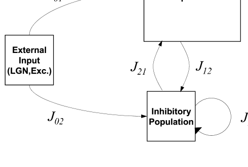
Figure 1: Structure of the model network.

The model network, indicated schematically in Fig. 1, consists of $N_{1}$ excitatory neurons and $N_{2}$ inhibitory ones. In this work we use leaky integrate-and-fire neurons, though the methods could be carried over directly to networks of other kinds of model neurons, such as conductance-based ones. They are randomly interconnected by synapses, both within and between populations, with the mean number of connections from population $b$ to population $a$ equal to $K_{b}$, independent of $a$. In specific calculations, we have used $K_{1}$ from 400 to 6400, and we take $K_{2}=K_{1}/4$. The population sizes $N_{a}$ do not enter directly in the mean field theory, only their ratios (the connection probabilities) $K_{a}/N_{a}$. We have used $K_{a}/N_{a}=0.1$ for both excitatory and inhibitory connections, implying $N_{1}=4N_{2}$.

We scale the synaptic strengths in the way van Vreeswijk and Sompolinsky did[4, 5], with each nonzero synapse from population $b$ to population $a$ having the value $J_{ab}/\sqrt{K_{b}}$. The parameters $J_{ab}$ are taken to be of order 1, so the net input current to a neuron from the $K_{b}$ neurons in population $b$ connected to it is of order $\sqrt{K_{b}}$. With this scaling, the fluctuations in this current are of order 1.

Similarly, we assume that the external input to any neuron is the sum of $K_{0}\gg 1$ contributions from individual neurons (in the LGN, if we are thinking about modeling V1), each of order $1/\sqrt{K_{0}}$, so the net input is of order $\sqrt{K_{0}}$. In our calculations, we have used $K_{0}=K_{1}$.

We point out that this scaling is just for convenience in thinking about the problem. In the balanced asynchronous firing state, the large excitatory and inhibitory input currents nearly cancel, leaving a net input current of order 1. Thus, for this choice, both the net mean current and its typical fluctuations are of order 1, which is convenient for analysis. The physiologically relevant assumptions are only that excitatory and inhibitory inputs are separately much larger than their sum and that the latter is of the same order as its fluctuations.

Our synapses are not modeled as conductances. Our synaptic strength simply defines the amplitude of the postsynaptic current pulse produced by a single presynaptic spike.

The model is formally specified by the sub-threshold equations of motion for the membrane potentials $u_{i}^{a}$ ($a=1,2$, $i=1,\ldots N_{a}$):

$$\frac{{\rm d}u_{i}^{a}}{{\rm d}t}=-\frac{u_{i}^{a}}{\tau}+\sum_{b=0}^{2}\sum_{j=1}^{N_{b}}J_{ij}^{ab}S_{j}^{b}(t),$$ (1)

together with the condition that when $u_{i}^{a}$ reaches the threshold $\theta_{a}$, the neuron spikes and the membrane potential is reset to a value $u_{r}^{a}$. The indices $a$ or $b=1$ or 2 label populations: $b=0$ refers to the (excitatory) population providing the external input, $a=1$ refers to the excitatory population and $a=2$ to the inhibitory population. In (1), $\tau$ is the membrane time constant (taken the same for all neurons, for convenience), the strength of the synapse from neuron $j$ in population $b$ to neuron $i$ in population $a$ is denoted by $J_{ij}^{ab}$, and $S_{i}^{b}(t)=\sum_{s}\delta(t-t_{jb}^{s})$ is the spike train of neuron $j$ in population $b$. We have ignored transmission delays, and we take the thresholds $\theta_{a}=1$ and the reset levels $u_{r}^{a}$ equal to the rest value of the membrane potential, 0. In our calculations, the thresholds are given a Gaussian distribution with a standard deviation equal to 10% of the mean. Analogous variability in other single-cell parameters (such as membrane time constants) could also be included in the model, but for simplicity we do not do so here.

We assume that the neurons in the external input population ($b=0$) fire as independent Poisson processes. However, the neurons in the network ($b=1,2$) are not in general Poissonian; it is their correlations that we want to find in this investigation.

Mean Field Theory: Stationary States

We describe the mean field theory and its computational implementation first for the case of stationary rates. When the connectivity is large and random, as we will assume here, each of the three terms in the sum on $b$ on the right-hand side of (1) can be treated as a Gaussian random function with time-independent mean. The simplest case is $b=0$, the external input. For simplicity, we assume that all $N_{0}$ neurons in the external population fire at the same rate, $r_{0}$. But because of the random connectivity, the net time-averaged input current they provide to a neuron in cortical population $a$ can vary from neuron to neuron. Assuming large, dilute connectivity ($K_{0}\gg 1$ and $K_{0}\ll N_{0}$), the central limit theorem then implies

$$\langle I_{i}^{a0}(t)\rangle=\sum_{j}J_{ij}^{a0}r_{0}=\sum_{j}(\overline{J_{ij}^{a0}}+\delta J_{ij}^{a0})r_{0}=J_{a0}r_{0}(\sqrt{K_{0}}+x_{i}^{a0}),$$ (2)

where $x_{i}^{a0}$ is a Gaussian-distributed random number of unit variance. By $\langle\cdots\rangle$ we mean a time average or, equivalently, an average over “trials” (independent repetitions of the Poisson processes defining the input population neurons). We will generally use a bar over a quantity to indicate an average over the neuronal population or over the distribution of the $J_{ij}^{ab}$. (Note that these two kinds of averages are very different things.)

Writing the spike train $S_{j}^{0}(t)$ for neuron $j$ in the input population as

$$S_{j}^{0}(t)=r_{0}+\delta S_{j}^{0}(t),$$ (3)

with $\langle\delta S_{j}^{0}(t)\rangle=0$, we can write the fluctuations around $\langle I_{i}^{a0}\rangle$ as

$$\delta I_{i}^{a0}(t)=\sum_{j}J_{ij}^{a0}\delta S_{j}^{0}(t)=J_{a0}\xi_{i}^{a0}(t)$$ (4)

where $\xi_{i}^{a0}(t)$ is white noise of power $r_{0}$:

$$\langle\xi_{i}^{a0}(t)\xi_{i}^{a0}(t^{\prime})\rangle=r_{0}\delta(t-t^{\prime})$$ (5)

Thus, quite generally, the input has a large mean value, of order $\sqrt{K_{0}}$, plus Gaussian fluctuations of order 1. The fluctuations are of two kinds. One is constant for a given neuron, independent of time and trial and arises from the fact that the connectivity is random and the neurons in the input population have a distribution of rates. The other fluctuation is a dynamical one, with correlations (independent of $i$) reflecting the Poisson dynamics of the input population neurons.

The recurrent input terms $I_{i}^{ab}(t)$ also have large means and fluctuations, static and dynamic, of order 1, but certain features of their statistics are slightly different, as a systematic formal derivation [7, 8] proves. Here we do not give the derivation, but just describe the result, which is that $I_{i}^{ab}(t)$ can be written

$$I_{i}^{ab}(t)=J_{ab}[\sqrt{K_{b}}r_{b}+B_{b}x_{i}^{ab}+\sqrt{1-K_{b}/N_{b}}\xi_{i}^{ab}(t)],$$ (6)

with

$$r_{b}=\overline{r_{j}^{b}}=\frac{1}{N_{b}}\sum_{j}r_{j}^{b}.$$ (7)

the average rate in population $b$, $x_{i}^{ab}$ a unit-variance Gaussian random number,

$$B_{b}=\sqrt{\left(1-\frac{K_{b}}{N_{b}}\right)\overline{(r_{j}^{b})^{2}}}$$ (8)

and

$$\langle\xi_{i}^{ab}(t)\xi_{i}^{ab}(t^{\prime})\rangle=C_{b}(t-t^{\prime}).$$ (9)

Here $C_{b}(t-t^{\prime})$ is the average autocorrelation function of the firing of neurons in population $b$,

$$C_{b}(t-t^{\prime})=\frac{1}{N_{b}}\sum_{j}\langle\delta S_{j}^{b}(t)\delta S_{j}^{b}(t^{\prime})\rangle,$$ (10)

with

$$\delta S_{j}^{b}(t)=S_{j}^{b}(t)-r_{j}^{b}.$$ (11)

Again, $x_{i}^{ab}$ is time- and trial-independent, while the noise $\xi_{i}^{ab}(t)$ varies both in time within a trial and randomly from trial to trial. Note that for this model a correct and complete mean field theory has to include rate fluctuations, through $\overline{(r_{j}^{b})^{2}}$, and the firing correlations, given by $C_{b}(t-t^{\prime})$, as well as the mean rates.

The means of the recurrent input currents $I_{i}^{ab}$ are completely analogous to the mean term in $I_{i}^{a0}$, but the effective noise is different in three ways

1. The amplitude $B_{b}$ of the static noise component (the second term) contains a factor of the rms rate $\sqrt{\overline{(r_{j}^{b})^{2}}}$, not $r_{b}$ as in (2). The same would be true for the static input noise ($b=0$) if we allowed a distribution of rates in the input population. So this difference is not an essential one. It occurs only because we made a simplifying assumption about the input population. However, we are not allowed to assume that about the neurons in the cortical network, which will always have a distribution of rates because of the random connectivity.

2. The neurons providing the source of these currents are not generally Poissonian, so their correlations appear in the statistics of the noise term.

3. The noise terms, both static and dynamic, have a factor $\sqrt{1-K_{b}/N_{b}}$ in front of them. This can be understood in the following way: It is the randomness in the synaptic connections in the network that generates these noise terms in the effective single-neuron problem; in general, they are proportional to $\overline{(\delta J_{ij}^{ab})^{2}}$, which is equal to $J_{ab}^{2}(1-K_{b}/N_{b})/N_{b}$ in our model. In the limit of full connectivity, $K_{b}=N_{b}$, all $J_{ij}^{ab}$ are equal and there is no randomness. Therefore there is no noise, as guaranteed here by this factor.

The self-consistency equations of mean field theory are simply the conditions that the average output statistics of the neurons, $r_{a}$, $\overline{(r_{j}^{a})^{2}}$ and $C_{a}(t-t^{\prime})$ are the same as those used to generate the inputs for single neurons using integrate-and-fire neurons with synaptic input currents given by (2), (4) and (6).

In an equivalent formulation, the second term in (6) can be omitted if the noise terms $\xi_{i}^{ab}(t)$ have correlations equal to the unsubtracted correlation function

$$C_{b}^{\rm tot}(t-t^{\prime})=\frac{1}{N_{b}}\sum_{j}\langle S_{j}^{b}(t)S_{j}^{b}(t^{\prime})\rangle$$ (12)

instead of (10). For $|t-t^{\prime}|\rightarrow\infty$, $C_{b}^{\rm tot}(t-t^{\prime})\rightarrow\overline{(r_{j}^{2})}$, so $\xi_{i}^{ab}(t)$ acquires a random static component of mean square value $\overline{(r_{j}^{b})^{2}}$.

In still another way to do it, one can use the square of the average rate, $r_{b}^{2}$ in place of $\overline{(r_{j}^{b})^{2}}$ in Eq.(8) for $B_{b}$ and employ noise with correlation function

$$\tilde{C}_{b}(t-t^{\prime})=\frac{1}{N_{b}}\sum_{j}\langle(S_{j}^{b}(t)-r_{b})(S_{j}^{b}(t^{\prime})-r_{b})\rangle.$$ (13)

For $|t-t^{\prime}|\rightarrow\infty$,

$$\tilde{C}_{b}(t-t^{\prime})\rightarrow\overline{(r_{j}^{b}-r_{b})^{2}}\equiv\overline{(\delta r_{j}^{b})^{2}}.$$ (14)

There are now two static random parts of $I_{i}^{ab}(t)$, one from the $B_{b}$ term and one from the static component of the noise. Their sum is a Gaussian random number with standard deviation equal to $B_{b}$ as given in (6). Thus these three ways of generating the input currents are all equivalent.

The balance condition

In a stationary, low-rate state, the mean membrane potential described by (1) has to be stationary. If excitation dominates, we have ${\rm d}u_{i}^{a}/{\rm d}t\propto\sqrt{K_{0}}$, implying a firing rate of order $\sqrt{K_{0}}$ (or one limited only by the refractory period of the neuron). If inhibition dominates, the neuron will never fire. The only way to have a stationary state at a low rate (less than one spike per membrane time constant) is to have the excitation and inhibition nearly cancel. Then the mean membrane potential can lie a little below threshold, and the neuron can fire occasionally due to the input current fluctuations. Thus, using (2) and (6), we have

$$\sum_{b=0}^{2}J_{ab}\sqrt{K_{b}}r_{b}={\cal O}(1)$$ (15)

or, up to corrections of ${\rm O}(1/\sqrt{K_{0}})$,

$$\sum_{b=0}^{2}\hat{J}_{ab}r_{b}=0$$ (16)

with $\hat{J}_{ab}=J_{ab}\sqrt{K_{b}/K_{0}}$. These are two linear equations in the two unknowns $r_{a}$, $a=1,2$, with the solution

$$r_{a}=\sum_{b=1}^{2}[{\sf\hat{J}}^{-1}]_{ab}J_{b0}r_{0},$$ (17)

where ${\sf\hat{J}}^{-1}$ is the inverse of the $2\times 2$ matrix with elements $\hat{J}_{ab}$, $a,b=1,2$. If there is a stationary balanced state, the average rates of the excitatory and inhibitory populations are given by (17) (in the large-$N$ limit).

This argument depends only on the rates, not on the correlations, and is exactly the same as that given by Amit and Brunel and by Sompolinsky and van Vreeswijk.

This calculation does not say whether this state is stable, however. To determine this, one can expand around this solution and examine the linear stability of the fluctuations, as done for their model by van Vreeswijk and Sompolinsky [5]. Here, we do not do this analytically, but rather check the stability of our states numerically within our algorithm.

Numerical procedure

For integrate-and-fire neurons in a stationary state, the mean field theory can be carried out analytically if a white-noise (Poisson firing) approximation is made [1, 2, 3]. But if firing correlations are to be taken into account, it is necessary to resort to numerical methods. Thus we simulate single neurons driven by Gaussian synaptic currents, collect their firing statistics to compute the rates $r_{a}$, rate fluctuations $\overline{(\delta r_{j}^{a})^{2}}$ and correlations $C_{a}(t-t^{\prime})$, and then use these to generate improved input current statistics. The cycle is repeated until the input and output statistics are consistent. This algorithm was first used by Eisfeller and Opper [23] to calculate the remanent magnetization of a mean field model for spin glasses.

Explicitly, we proceed as follows. We simulate single excitatory and inhibitory neurons over “trials” 100 integration timesteps long. (We will call each timestep a “millisecond”. We have explored using smaller timesteps and verified that there are no qualitative changes in the results.) We start from estimates of the rates given by the balance condition, which makes the net mean input current vanish. Then the sum of the ${\cal O}(\sqrt{K_{b}})$ terms in (2) and (6) vanishes, leaving only the rate fluctuation and noise terms. We then run 10000 trials of single excitatory and inhibitory neurons, selecting on each trial random values of $x_{i}^{ab}$ and $\xi_{i}^{ab}(t)$. Since at this point we do not have any estimates of either the rate fluctuations $\overline{(\delta r_{j}^{b})^{2}}$ or the correlations $C_{b}(t-t^{\prime})$, we use $r_{b}^{2}$ in place of $\overline{(r_{j}^{b})^{2}}$ in Eq.(8)for $B_{b}$ and use white noise for $\xi_{i}^{ab}(t)$: $C_{b}(t-t^{\prime})\rightarrow r_{b}\delta(t-t^{\prime})$.

The random choice of $x_{i}$ from trial to trial effectively samples across the neuronal populations, so we can then collect the statistics $r_{a}$, $\overline{(r_{j}^{a})^{2}}$ (or, equivalently, $\overline{(\delta r_{j}^{a})^{2}}$), and $C_{a}(t-t^{\prime})$ from these trials. These can be used to generate an improved estimate of the input noise statistics to be used in (6) in a second set of trials, which yields new spike statistics again. This procedure is iterated until the input and output statistics agree. This may take up to several hundred iterations, depending on network parameters and how the computation is organized.

If one tries this procedure in its naive form, i.e., using the output statistics directly to generate the input noise at the next step, it will lead to big oscillations and not converge. It is necessary to make small corrections (of relative order $1/K_{0}$) to the previous input noise statistics to guarantee convergence.

When one computes statistics from the trials in any iteration, the simplest procedure involves calculating not (10), but rather $\tilde{C}_{b}(t-t^{\prime})$ (Eq.(13)). From it, we can proceed in two ways. In the first, from its $|t-t^{\prime}|\rightarrow\infty$ limit we can obtain $\overline{(\delta r_{j}^{b})^{2}}$, and thereby $\overline{(r_{j}^{b})^{2}}=r_{b}^{2}+\overline{(\delta r_{j}^{b})^{2}}$ for use in calculating $B_{b}$ in (8). Subtracting this limiting value from $\tilde{C}_{b}(t-t^{\prime})$ give us $C_{b}(t-t^{\prime})$ (which vanishes for large $|t-t^{\prime}|$) for use in generating the noise $\xi_{i}^{ab}(t)$. This is the first of the three methods described above.

Alternatively, we can use the third method: At each step of our iterative procedure we can generate noise directly with the correlations $\tilde{C}_{b}(t-t^{\prime})$ (which are long-ranged in time) and use $r_{b}^{2}$ in place of $\overline{(r_{j}^{b})^{2}}$ in calculating $B_{b}$ (8). We have verified that the two methods give the same results when carried out numerically, though the second procedure converges more slowly.

While the true rates in the stationary case are time-independent and $C_{a}(t,t^{\prime})$ is a function only of $t-t^{\prime}$, the statistics collected over a finite set of noise-driven trials will not exactly have these stationarity properties. Therefore we improve the statistics and impose time-translational invariance by averaging the measured $r_{a}(t)$ and $\overline{(\delta r_{j}^{a}(t))^{2}}$ over $t$ and averaging over the measured values $C_{a}(t,t^{\prime})$ with a fixed $t-t^{\prime}$.

After the iterative procedure converges, so that we have a good estimate of the statistics of the input, we want to run many trials on a single neuron and compute its firing statistics. This means that the numbers $x_{i}^{ab}$ ($b=0,1,2$) should be held constant over these trials. In this case it is necessary to subtract out the large $t-t^{\prime}$ limit of $\tilde{C}_{a}(t-t^{\prime})$ and use fixed $x_{i}^{ab}$ (constant in time and across trials) to generate the input noise. (If we did it the other way, without the subtraction, we would effectively be assuming that $x_{i}^{ab}$ changed randomly from trial to trial, which is not correct.)

In our calculations we have used 10000 trials to calculate these single-neuron firing statistics. We perform the subtraction of the long-time limit of $\tilde{C}_{a}(t-t^{\prime})$ at $|t-t^{\prime}|=50$, and we have checked that (13) is flat beyond this point in all the cases we have done.

If we perform this kind of measurement separately for many values of the $x_{i}^{ab}$, we will be able to see how the firing statistics vary across the population. Here, however, we will confine most of our attention to what we call the “average neuron”: the one with the average value (0) of all three $x_{i}^{ab}$.

In particular, we calculate the mean spike count in the 100-ms trials and its variance across trials. From this we can get the Fano factor $F$ (the variance/mean ratio). We also compute the autocorrelation function, which offers a consistency check, since the Fano factor can also be obtained from

$$F=\frac{1}{r}\int_{-\infty}^{\infty}C(\tau){\rm d}\tau.$$ (18)

(This formula is valid when the measurement period is much larger than the time over which $C(\tau)$ falls to zero.)

We will study below how these firing statistics vary as we change various parameters of the model: the input rates $r_{0}$, parameters that control the balance of excitation and inhibition, and the overall strength of the synapses. This will give us some generic understanding of what controls the degree of irregularity of the neuronal firing.

Nonstationary Case

When the input population is not firing at a constant rate, almost the same calculational procedure can be followed, except that one does not average measured rates, their fluctuations or correlation function over time. To start out, we get initial instantaneous rate estimates from the balance condition, assuming that the time-dependent average input currents do not vary too quickly. (This condition is not very stringent; van Vreeswijk and Sompolinsky showed that the stability eigenvalues are proportional to $\sqrt{K_{0}}$, so if they have the right sign the convergence to the balanced state is very rapid.)

To do the iterative procedure to satisfy the self-consistency conditions of the theory, it is simplest to use the second of the two ways described above (not doing any subtraction until the final calculations with single neurons). In this case the expression (8) does not include rate fluctuations, and we get equations for the noise input currents just like (2), (4) and (6) except that the $r_{b}$ are $t$-dependent and the correlation functions $C_{b}$ and $D_{b}$ depend on both $t$ and $t^{\prime}$, not just their difference.

The only tricky part is the subtraction of the long-time limit of the correlation function, which is not simply defined.

We treat this problem in the following way. We examine the rate-normalized quantity

$$\hat{D}_{a}(t,t^{\prime})=\frac{D_{a}(t,t^{\prime})}{r_{a}(t)r_{a}(t^{\prime})}.$$ (19)

We find that this quantity is time-translation invariant (i.e., a function only of $t-t^{\prime}$) to a very good approximation, so we perform the subtraction of the long-time limit on it. Then multiplying the subtracted $\hat{D}$ by $r_{a}(t)r_{a}(t^{\prime})$ gives a good approximation to the true correlation function $C_{a}(t,t^{\prime})$. The meaning of this finding is, loosely speaking, that when the rates vary (slowly enough) in time, the correlation functions just inherit these rates as overall factors without changing anything else about the problem.

We will use the this time-dependent formulation below to simulate experiments like those of Gershon et al [17], where the LGN input $r_{0}(t)$ to visual cortical cells is time-dependent because of the flashing-on and off of the stimulus.

3 Results

The results presented in this chapter were obtained from simulations with parameters corresponding to population sizes of $N_{1}=$ 40,000 excitatory neurons and $N_{2}=$ 10,000 inhibitory neurons. With the above mentioned connection probabilities of $K_{a}/N_{a}=0.1$, this translates to an average number of $K_{1}=4000$ excitatory inputs and $K_{2}=1000$ inhibitory inputs to each neuron. The average number of external (excitatory) inputs $K_{0}$ was chosen to be equal to $K_{2}$. All neurons have the same membrane time constant $\tau$ of $10$ ms.

To study the effect of various combinations in synaptic strength, we use the following generic form to define the intra-cortical weights $J_{ab}$:

$$\left(\begin{array}[]{cc}J_{11}&J_{12}\\ J_{21}&J_{22}\end{array}\right)=\left(\begin{array}[]{cc}\epsilon&-2g\\ 1&-2g\end{array}\right)$$ (20)

For the synaptic strengths from the external population we use $J_{10}=1$ and $J_{20}=\epsilon$. With this notation, $g$ determines the strength of inhibition relative to excitation within the network, and $\epsilon$ the strength of intracortical excitation. Additionally, we scale the overall strength of the synapses with a multiplicative scaling factor denoted $J_{s}$ so that each synapse has an actual weight of $J_{s}\cdot J_{ab}$, regardless of $a$ and $b$.

Figure 2: Fano factors as a function of overall synaptic strength $J_{s}$ and intracortical excitation strength $\epsilon$ for three different inhibition factors: $g=1$, $1.5$, and $2$, respectively. The increase of any of these parameters results in more irregular firing statistics as measured by the Fano factor.

Figure 2 summarizes how the firing firing statistics depend on all of the parameters $g$, $\epsilon$, and $J_{s}$. The irregularity of spiking, as measured by the Fano factor, depends most sensitively on the overall scaling of the synaptic strength, $J_{s}$. The Fano factor increases systematically as $J_{s}$ increases, and higher values of intracortical excitation $\epsilon$ also result in higher values of $F$. The same pattern holds for stronger intracortical inhibition, parameterized by $g$. For all of these cases the mean firing rate remains virtually unchanged due to the dynamic balance of excitation and inhibition in the network, whereas the fluctuations increase with the increase of any of the synaptic weights.

Figure 3: Interspike interval distributions for fixed $\epsilon=0.5$ and $g=1$, and three different values of overall synaptic strength $J_{s}$: $1.5$ (superpoissonian), $0.75$ (Poissonian), and $0.375$ (subpoissonian). Overlayed on each figure is the exponential fall-off of a true Poisson distribution with the same average rate as in all of the three cases.

Interspike interval (ISI) distributions are shown in Figure 3 for three different values of $J_{s}$, keeping $\epsilon$ and $g$ fixed at $0.5$ and $1$, respectively. For a Poisson spike train, the Fano factor $F=1$, while $F>1$ (which we term “superpoissonian”) indicates a tendency of spikes occurring in clusters separated by accordingly longer empty intervals, and $F<1$ (“subpoissonian”) indicates more regularity, reflected by a narrower distribution. We have adjusted the input rate $r_{0}$ so that the output rate is the same in all three cases.

The top panel of Figure 3 shows the ISI distribution of a superpoissonian spike train, obtained for $J_{s}=1.5$. Overlayed on the histogram of ISI counts is an exponential curve indicating a Poisson distribution with the same mean ISI length. Compared with the Poisson distribution, the superpoissonian spike train contains more short intervals, as seen by the peak at short lengths, and also more long intervals, causing a long tail. Necessarily, the interval count around the average ISI length is lower than that for a Poisson spike train.

The ISI distribution in the middle panel of Figure 3 belongs to a spike train with a Fano factor close to one, obtained for $J_{s}=0.75$. The overlayed exponential reveals a deviation from the ISI count: while intervals of diminishing length are the most likely ones for a real Poisson process, our neuronal spike trains always show some refractoriness reflected by a dip at the shortest intervals. (We have not used an explicit refractory period in our model. The dip seen here simply reflects the fact that it takes a little time for the membrane potential distribution to return to its steady-state form after reset.) Apart from this deviation, however, there is a close resemblance between the observed distribution and the “predicted” one.

Finally, the lower panel of Figure 3 depicts a case with $F<1$, with weaker synapses, leading to a stronger refractory effect and (since the rate is fixed) an accordingly narrower distribution around the average ISI length, as compared to the overlayed Poisson distribution. This distribution was obtained with weak synapses produced by a small scaling factor of $J_{s}=0.375$.

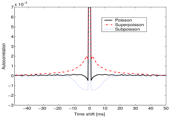
Figure 4: Three different spike train autocorrelations illustrating the relationship between the Fano factor $F$ and the area under the curve. For $F=1$ (Poissonian, black solid line), the autocorrelation is an almost perfect delta function. $F>1$ (superpoissonian, red dash-dot line) is reflected by a hill generating a positive area, and $F<1$ (subpoissonian, blue dotted line) is accompanied by a valley of negative correlations. (See the text for more details.)

As mentioned in the previous section, the Fano factor can also be obtained by integrating over the spike train autocorrelation divided by the spike rate (18). For a Poisson process the autocorrelation vanishes for all lags different from zero. In contrast, $F>1$ (superpoissonian case) implies a positive integral over non-zero lags, whereas in the subpoissonian case there must be a negative area under the curve. Figure 4 shows examples of autocorrelations for all of the three cases. For the superpoissonian case (red dash-dot line), there is a “hill” of positive correlations for short intervals, reflecting the tendency toward spike clustering. The subpoissonian autocorrelation (blue dotted line) shows a valley of negative correlations for short intervals, indicating well separated spikes in a more regular spike train. The curve labeled as Poisson (black solid line) does have a small valley around zero lag, which reflects once more the refractoriness of neurons to fire at extremely short intervals, unlike a completely random Poisson process. (Actually, the measured $F$ in this case is slightly greater than 1, implying that in this case the integral of the very small positive tail for $t>2$ ms is slightly larger than that of the (more obvious) negative short-time dip.)

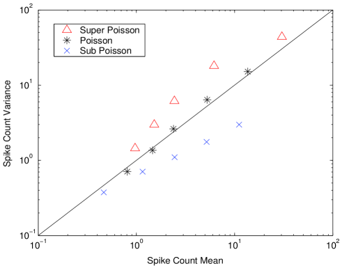
Figure 5: Spike count log(variance) vs. log(mean) for three different values of overall synaptic strength $J_{s}$, varying the external input rate $r_{0}$. For $J_{s}=1.25$ (superpoissonian, red triangles) the data look qualitatively like those from experiments. The other values for $J_{s}$ are $0.75$ (Poisson, black stars) and $0.375$ (subpoissonian, blue crosses).

Measurements on V1 neurons in awake monkeys (see for example Gershon et al. [17]) suggest a linear relationship between the log variance and the log mean of stimulus-elicited spike counts. We find a similar dependence for neurons within our model network. Figure 5 shows results for three different values of $J_{s}$. In each case, five different values of the external input rate $r_{0}$ were tried, causing various mean spike counts and variances. The logarithm of the spike count variance is plotted as a function of the logarithm of the spike count mean, and a solid diagonal line indicates the identity, i.e, a Fano factor of exactly 1. We see that for the largest value of $J_{s}$ used here, the data look qualitatively like those from experiments, with Fano factors in the range around 1.5 to 2.

Nonstationary Case

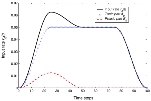
Figure 6: Parametrization of the time-dependent input rate $r_{0}(t)$. The input is modeled as the sum of three functions: (1) a stationary background rate (which is zero in this case); (2) a tonic part, which rises within the first 20 ms to a constant level of $A_{0}$ where it stays for 60 ms, falling back to zero within the last 20 ms; and (3) an initial phasic part, which is nonzero only in the first 50 ms, rising to a maximum value of $B_{0}$.

The results presented in the previous section were obtained with stationary inputs, while experimental data like those from [17] were collected from visual neurons subject to time-dependent inputs. Therefore, we performed calculations of the spike statistics in which the input population rate $r_{0}$ was time-dependent. The modeled temporal shape of $r_{0}(t)$ is depicted in Figure 6. It is the sum of three terms:

$$r_{0}(t)=R_{0}+A(t)+B(t)$$ (21)

The first, $R_{0}$, is just a constant, as in the preceding section. The second term, $A(t)$, rises to a maximum over a 25-ms interval, remains constant for 50 ms, and then falls off to zero over the final 25 ms.

$$A(t)=\left\{\begin{array}[]{ll}0.5A_{0}(1-\cos(4t\pi/T))&\hbox{for $0<t\leq T/4$}\\ A_{0}&\hbox{for $T/4<t\leq 3T/4$}\\ 0.5A_{0}(1-\cos(4(T-t)\pi/T))&\hbox{for $3T/4<t\leq T$,}\\ \end{array}\right.$$ (22)

where $T$ is the total simulation interval of 100 ms. The third term, $B_{0}$, rises to a maximum in the first 25 ms and then falls back to zero in the next 25 ms, remaining zero thereafter.

$$B(t)=\left\{\begin{array}[]{ll}0.5B_{0}(1-\cos(4t\pi/T))&\hbox{for $0<t\leq T/4$}\\ 0.5B_{0}(1-\cos(4(T/2-t)\pi/T))&\hbox{for $T/4<t\leq T/2$}\\ 0&\hbox{for $T/2<t\leq T$.}\\ \end{array}\right.$$ (23)

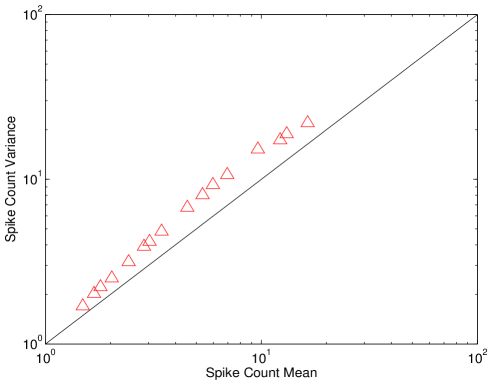
Figure 7: Spike count log(variance) vs. log(mean) for time-varying external inputs with varying overall strength. The neuron in the simulated network (red triangles) fires in a superpoissonian regime, with an almost linear relationship for low spike rates between the log variance and the log mean, resembling closely data obtained from in-vivo experiments. The diagonal solid line indicates the identity of variance and mean (Fano factor $F=1$).

Figure 7 shows the logarithm of the spike count variance plotted against the logarithm of the spike count mean for various non-stationary inputs characterized by different values of $A_{0}$ and $B_{0}$. The graph shows results for $J_{s}=1$, $\epsilon=0.5$, $g=1$, and a background rate of $R_{0}=0.1$. Table 1 shows the choice of the sixteen combinations of the stimulus parameters $A_{0}$ and $B_{0}$, together with the resulting Fano factors $F$ for the simulated neuron.

$A_{0}$	$0.375$	$0.375$	$0.500$	$0.500$	$0.750$	$0.750$	$1.000$	$1.000$
$B_{0}$	$0.125$	$0.375$	$0.125$	$0.375$	$0.250$	$0.750$	$0.250$	$0.750$
$F$	$1.14$	$1.2$	$1.22$	$1.23$	$1.29$	$1.36$	$1.37$	$1.4$

$A_{0}$	$1.500$	$1.500$	$2.000$	$2.000$	$3.000$	$3.000$	$4.000$	$4.000$
$B_{0}$	$0.500$	$1.500$	$0.500$	$1.500$	$1.000$	$3.000$	$1.000$	$3.000$
$F$	$1.48$	$1.5$	$1.55$	$1.53$	$1.57$	$1.41$	$1.43$	$1.34$

Table 1: Stimulus parameters $A_{0}$ and $B_{0}$ for the results depicted in Figure 7, and the resulting Fano factors $F$.

The data look qualitatively like those obtained from in-vivo experiments [17] and are similar to the superpoissonian case in Figure 5. The neuron fires consistently in a superpoissonian regime with Fano factors slightly higher than 1 and an almost linear relationship between the log variance and the log mean for low spike counts. For higher spike counts, the curve bends towards values of lower Fano factors, just as for stationary inputs (Figure 5). In both cases, this bend reflects the the decrease in irregularity of firing caused by an increasingly prominent role of refractoriness for shorter interspike intervals.

4 Discussion

Cortical neurons receive thousands of both excitatory and inhibitory inputs, and despite the high number of inputs from nearby neurons with similar firing statistics and similar connectivity, their observed firing is very irregular [9, 10, 11, 12, 13, 14, 15, 16, 17, 18, 19, 20, 21]. Dynamically balanced excitation and inhibition through a simple feedback mechanism provides an explanation that naturally accounts for this phenomenon without requiring fine tuning of the parameters [1, 2, 3, 4, 5]. Moreover, neurons in such model networks show an almost linear input-output relationship (input current versus firing frequency), as do neurons in the neocortex.

Here, we have extended the mean-field description of the dynamically balanced asynchronous firing state to analyze firing correlations. We found that the relationship between the observed irregularity of firing (spike count variance) and the firing rate (spike count mean) of the neurons resemble closely data collected from in-vivo experiments (see Figures 5 and 6). To do this, we developed a complete mean-field theory for a network of leaky integrate-and-fire neurons, in which both firing rates and correlation functions are determined self-consistently. Using an algorithm that allows us to find the solutions to the mean-field equations numerically, we could elucidate how the strength of synapses within the network influences the expected firing statistics of cortical neurons in a systematic manner (see Figure 2).

We have shown that the irregularity of firing, as measured by the Fano factor, increases with increasing synaptic strengths (Figure 2). Nearly Poisson statistics (with $F\approx 1$) are observed for moderately strong strengths, but the transition from subpoissonian to superpoissonian statistics is smooth, without a special role for $F=1$.

The higher irregularity in the spike counts is always accompanied by a tendency toward more “bursty” firing. (These bursts are a network effect; the model contains only leaky integrate-and-fire neurons, which do not burst on their own.) This burstiness can best be seen in the spike train autocorrelation function (Figure 4), which acquires a hill of growing size and width around zero lag for increasing Fano factors. The interdependence between firing irregularity and bursting can be understood with help of the ISI distributions depicted in Figure 3: when the rate, and thus the average ISI, is kept constant, then any higher count for shorter-than-average ISIs must be accompanied by an accordingly higher count for longer ISIs (indicating bursts), and vice versa. Thus higher irregularity always goes hand in hand with a higher tendency toward temporal clustering of spikes.

Why do stronger synapses lead to higher irregularity in firing? The size of the input current fluctuations in (6) are controlled by the $J_{ab}$, and so, therefore, are the corresponding membrane potential fluctuations. Thus, for example, the width of the steady-state membrane potential distribution is proportional to $J_{s}$. We next have to consider where this distribution is centered. Remembering that, according to the balance condition, the firing rate is independent of $J_{s}$, the center of the distribution has to move farther away from threshold as $J_{s}$ is increased in order to keep the rate fixed. Therefore, for very small $J_{s}$ almost the entire equilibrium membrane potential distribution will lie well above the post-spike reset value, while for large $J_{s}$ it will be mostly below reset.

Immediately after a spike, the membrane potential distribution is a delta-function centered at the reset (here 0). It then spreads and its mean moves up or down toward its equilibrium value. This equilibration will take about a membrane time constant. If the equilibrium value is well above zero (the small-$J_{s}$ case), the probability of reaching threshold will be suppressed during this time, implying a refractory dip in the ISI distribution and the correlation function and a tendency toward a Fano factor less than 1.

In the large-$J_{s}$ case, on the other hand, where the membrane potential is reset much closer to the threshold than to its eventual equilibrium value, the initial rapid spread (with the width growing proportional to $J_{s}\sqrt{t}$) leads to an enhanced probability of early spikes. At short times this diffusive spread dominates the downward drift of the mean (which is only linear in $t$). Thus there is extra weight in the ISI distribution and a positive correlation function at these short times, leading to a Fano factor greater than 1.

Empirically, an approximate power-law relationship between the mean and variance of the spike count has frequently been observed for cortical neurons (see, e.g., [11, 13, 17, 20]). Our model shows the same qualitative feature (Figures 5 and 6), though we have no argument that the relation should be an exact power law. However, this agreement suggests that the model captures at least part of physics underlying the firing statistics.

As already observed, not all of the variability in measured neuron responses has to be explained in the manner outlined above. Changing conditions during the run of a single experiment may introduce extra irregularity, caused by collecting statistics over trials with different mean firing rates. The present analysis shows why – and how much – irregularity can be expected due to intrinsic cortical dynamics.

Our formulation of the mean-field theory is general enough to allow straightforward extensions to greater biological realism and to more complicated network architectures. We have introduced a generalization of this model with conductance-based synapses in another paper [24]. We have also extended the model to include systematic structure in the connections, modeling an orientation hypercolumn in the primary visual cortex [25]. Moreover, our algorithm for finding the mean-field solutions is not restricted to networks of integrate-and-fire neurons. It can be applied to any kind of neuronal model. Furthermore, any kind of synaptic dynamics can be incorporated by using synaptically filtered spike trains to compute the self-consistent solutions.

References

- [1] D Amit and N Brunel, Model of spontaneous activity and local structured activity during delay periods in the cerebral cortex. Cereb Cortex 7, 237-252 (1997)
- [2] D Amit and N Brunel, Dynamics of a recurrent network of spiking neurons before and following learning. Network 8, 373-404 (1997)
- [3] N Brunel, Dynamics of sparsely connected networks of excitatory and inhibitory spiking neurons. J Comput Neurosci 8, 183-208 (2000)
- [4] C van Vreeswijk and H Sompolinsky, Chaos in neuronal networks with balanced excitatory and inhibitory activity. Science 274, 1724-1726 (1996)
- [5] C van Vreeswijk and H Sompolinsky, Chaotic balanced state in a model of cortical circuits. Neural Comp 10, 1321-1371 (1998)
- [6] M W Oram, M C Wiener, R Lestienne and B J Richmond, Stochastic nature of precisely-timed spike patterns in visual system neural responses. J Neurophysiol 81, 3021-3033 (1999)
- [7] C Fulvi Mari, Random networks of spiking neurons: instability in the xenopus tadpole moto-neuron pattern. Phys Rev Lett 85, 210-213 (2000)
- [8] R Kree and A Zippelius, Continuous-time dynamics of asymmetrically diluted neural networks. Phys Rev A 36, 4421-4427 (1987)
- [9] P Heggelund and K Albus, Response variability and orientation discrimination of single cells in in striate cortex of cat. Exp Brain Res 32, 197-211 (1978)
- [10] A F Dean, The variability of discharge of simple cells in the cat striate cortex. Exp Brain Res 44, 437-440 (1981)
- [11] D J Tolhurst, J A Movshon and I D Thompson, The dependence of response amplitude and variance of cat visual cortical neurones on stimulus contrast. Exp Brain Res 41, 414-419 (1981)
- [12] D J Tolhurst, J A Movshon and A F Dean, The statistical reliability of signals in single neurons in cat and monkey visual cortex. Vision Res 23, 775-785 (1983)
- [13] R Vogels, W Spileers and G A Orban, The response variability of striate cortical neurons in the behaving monkey. Exp Brain Res 77, 432-436 (1989)
- [14] R J Snowden, S Treue and R A Andersen, The response of neurons in areas V1 and MT of the alert rhesus monkey to moving random dot patterns. Exp Brain Res 88, 389-400 (1992)
- [15] M Gur, A Beylin and D M Snodderly, Response variability of neurons in primary visual cortex (V1) of alert monkeys. J Neurosci 17, 2914-2920 (1997)
- [16] M N Shadlen and W T Newsome, The variable discharge of cortical neurons: implications for connectivity, computation, and information coding. J Neurosci 18, 3870-3896 (1998)
- [17] E Gershon, M C Wiener, P E Latham and B J Richmond, Coding strategies in monkey V1 and inferior temporal cortex. J Neurophysiol 79, 1135-1144 (1998)
- [18] P Kara, P Reinagel and R C Reid, Low response variability in simultaneously recorded retinal, thalamic, and cortical neurons. Neuron 27,635-646 (2000)
- [19] G T Buracas, A M Zador, M R DeWeese and T D Albright, Efficient discrimination of temporal patterns by motion-sensitive neurons in primate visual cortex. Neuron 20, 959-969 (1998)
- [20] D Lee, N L Port, W Kruse and A P Georgopoulos, Variability and correlated noise in the discharge of neurons in motor and parietal areas of primate cortex. J Neurosci 18, 1161-1170 (1998)
- [21] M R DeWeese, M Wehr and A M Zador, Binary spiking in auditory cortex. J Neurosci 23, 7940-7949 (2003)
- [22] J Hertz, B Richmond and K Nilsen, Anomalous response variability in a balanced cortical network model. Neurocomputing 52–54, 787–792 (2003)
- [23] H Eisfeller and M Opper, New method for studying the dynamics of disordered spin systems without finite-size effects. Phys Rev Lett 68, 2094-2097 (1992)
- [24] A Lerchner, M Ahmadi and J Hertz, High conductance states in a mean field cortical network model. CNS 2003, to be published in Neurocomputing (2004)
- [25] J Hertz and G Sterner, Mean field model of an orientation hypercolumn. Program No. 911.19 Abstract Society for Neuroscience (2003)