Kinetics of protein-DNA interaction: facilitated target location in sequence-dependent potential

Abstract

Recognition and binding of specific sites on DNA by proteins is central for many cellular functions such as transcription, replication, and recombination. In the process of recognition, a protein rapidly searches for its specific site on a long DNA molecule and then strongly binds this site. Here we aim to find a mechanism that can provide both a fast search (1-10 sec) and high stability of the specific protein-DNA complex ($K_{d}=10^{-15}-10^{-8}$ M).

Earlier studies have suggested that rapid search involves the sliding of a protein along the DNA. Here we consider sliding as a one-dimensional (1D) diffusion in a sequence-dependent rough energy landscape. We demonstrate that, in spite of the landscape’s roughness, rapid search can be achieved if 1D sliding is accompanied by 3D diffusion. We estimate the range of the specific and non-specific DNA-binding energy required for rapid search and suggest experiments that can test our mechanism. We show that optimal search requires a protein to spend half of time sliding along the DNA and half diffusing in 3D. We also establish that, paradoxically, realistic energy functions cannot provide both rapid search and strong binding of a rigid protein. To reconcile these two fundamental requirements we propose a search-and-fold mechanism that involves the coupling of protein binding and partial protein folding.

Proposed mechanism has several important biological implications for search in the presence of other proteins and nucleosomes, simultaneous search by several proteins etc. Proposed mechanism also provides a new framework for interpretation of experimental and structural data on protein-DNA interactions.

I Introduction

The complex transcription machinery of cells is primarily regulated by a set of proteins, transcription factors (TFs), that bind DNA at specific sites. Every TF can have from one to several dozens of such specific sites on the DNA. Upon binding to the site, TF forms a stable protein-DNA complex that can either activate or repress transcription of nearby genes, depending on the actual control mechanism. Fast and reliable regulation of gene expression requires (1) fast ($\sim$1-10 sec) search and recognition of the specific site (referred to as the target or cognate site below) out of $10^{6}$ - $10^{9}$ possible sites on the DNA, and (2) stability of the protein-DNA complex ($K_{d}=10^{-15}-10^{-8}$ M). In spite of its apparent simplicity, such a mechanism is not understood in depth, either qualitatively or quantitatively. Here we focus on a simpler case of bacterial TFs recognizing their cognate (target) sites on the naked DNA. Needless to say that eukaryotic protein-DNA recognition is significantly complicated by chromatin packing of the DNA and multi-subunit structure of TFs. Interestingly, similar problems of specific binding and binding rate arises in the context of oligonucleotides-DNA binding Lomakin and Frank-Kamenetskii (1998)

Vast amounts of experimental data available these days provide the structures of protein-DNA complexes at atomic resolution in crystals and in solution Luscombe et al. (2000); Bell and Lewis (2001, 2000); Lewis et al. (1996); Schumacher et al. (1994), binding constants for dozens of native and hundreds of mutated proteins Takeda et al. (1989); Grillo et al. (1999), calorimetry measurements Spolar and Record (1994), and novel single-molecule experiments Shimamoto (1999). These experimental data contributed most significantly to our present understanding of protein-DNA interaction since the early work of von Hippel, Berg $et.~{}al.$ In a series of pioneering articles Berg et al. (1981); Winter et al. (1989); von Hippel and Berg (1989); Berg and von Hippel (1987), they have created a conceptual basis for describing of both the kinetics and thermodynamics of protein-DNA interaction, which became a starting point for practically every subsequent theoretical work on the subject.

We start by reviewing the history of the problem and describing the paradox of the ”faster than diffusion” association rate. Next, we present the classical model of protein-DNA ”sliding” and explain how this model can resolve the paradox. We outline the problem that the sliding mechanism faces if the energetics of protein-DNA interactions are taken into account. Next we introduce our novel quantitative formalism and undertake in-depth exploration of possible mechanisms of protein-DNA interaction.

I.1 ”Faster than diffusion” search

The problem of how a protein finds its target site on DNA has a long history. In 1970, Riggs et. al. Riggs et al. (1970b, a) measured the association rate of LacI repressor and its operator on DNA as $\sim 10^{10}$ M^-1s^-1. This astonishingly high rate (as compared to other biological binding rates) was shown to be much higher than the maximal rate achievable by 3D diffusion. In fact, if a protein binds its site by 3D diffusion, it has to hit the right site on the DNA within $b=0.34~{}$nm. (A shift by $0.34~{}$nm would result in binding a site that is different from the native one by 1bp. Such a site can be very different, e.g. GCGCAATT vs CGCAATTC). Using the Debye-Smoluchowski equation for the maximal rate of a bimolecular reaction (see e. g. Richter and Eigen (1974); Flyvbjerg et al. (2002); Bruinsma (2002)), with a protein diffusion coefficient of $D_{3d}\sim 10^{-7}$cm${}^{2}/$s Elowitz et al. (1999) we get

$$k_{DS}=4\pi D_{3D}b\sim 10^{8}~{}\mbox{M}^{-1}\mbox{s}^{-1}$$ (1)

This value for the association rate, relevant for in vitro measurements, corresponds to target location in vivo on a time scale of a few seconds, when each cell contains up to several tens of TF molecules.

To resolve the discrepancy between the experimentally measured rate of $10^{10}$ M^-1s^-1 and the maximal rate of $10^{8}$ M^-1s^-1 allowed by diffusion, Riggs et. al., Richter et. al. Richter and Eigen (1974) and later Winter, Berg and von Hippel Berg et al. (1981); von Hippel and Berg (1989) suggested that the dimensionality of the problem changes during the search process. They concluded that while searching for its target site, the protein periodically scans the DNA by “sliding” along it.

I.2 Sliding along the DNA

If a protein performs both 3D and 1D diffusion, then the total search process can be considered as a 3D search followed by binding DNA and a round of 1D diffusion. Upon dissociation from the DNA, the protein continues 3D diffusion until it binds DNA in a different place, and so on. Some experimental evidence supports this search mechanism. These include affinity of the DNA-binding proteins for any fragment of DNA (non-specific binding), single molecule experiments where 1D diffusion has been observed and visualized, and numerous other experiments where the rate of specific binding to the target site has been significantly increased by lengthening non-specific DNA surrounding the site Kim et al. (1987). What are the benefits and the mechanism of 1D diffusion and what limits the search rate?

Here we address this question and consider possible search mechanisms that involve both 1D and 3D diffusion, where 1D diffusion along the DNA proceeds along the rough energy landscape. Quantitative analysis of the search process brought us to the following four main results:

• When the roughness of the binding energy landscape is greater than ${\sim 2k_{B}T}$, the diffusion along the DNA becomes extremely slow with the protein unable to diffuse more than a few base-pairs. The total search process is prohibitively slow.

• If the search proceeds by a combination of 1D and 3D diffusion, non-specific binding to the DNA plays a very important role in controlling the balance between these two processes. The optimal energy of non-specific binding can provide the maximal search rate. Although faster than either 3D or 1D search alone, optimal combination of 3D and 1D diffusion cannot expedite the search if the roughness of the landscape is greater than $\sim 2k_{B}T$.

• Experimentally observed and biologically relevant rates of search can be reached only when 1D sliding proceeds through a fairly smooth landscape with a roughness of the order of $k_{B}T$.

• Paradoxically, the stability of the protein-DNA complex at the target site requires a roughness of the binding energy landscape considerably larger than $k_{B}T$. Rapid search, however, by 1D/3D diffusion is impossible at such roughness.

Finally, we formulate this “search speed–stability” paradox and suggest a search-and-fold mechanism that can resolve it. The paradox can be resolved if the DNA-binding protein has two distinct (conformational) states in which it exhibits two modes of binding. In the first, mode that has weaker binding and a smother landscape, it searches for its site. In the second recognition mode, that has larger roughness of the binding landscape, the protein tightly binds DNA sites. Correlation between the energy landscapes in the two modes and the energy difference and the barrier between the two protein conformations control the frequency of transition between the two modes and provides effective pre-selection of low-energy sites.

We suggest that these modes correspond to two distinct conformational states of the protein-DNA complex (a more open complex in the search mode, and a more tight one in the recognition mode). Transition between the two states can include partial folding of the protein, water extrusion, change in the DNA conformation etc. Focusing on the conformation of the protein, and without loss of generality, we consider a partially unfolded (disordered) conformation and the folded conformation bound to the cognate site as the two conformations required by our model. In fact, a protein in the partially unfolded conformation may have fewer and/or weaker interactions with DNA allowing rapid sliding. Folded conformation, in turn, provides stronger and more specific interactions required for for tight binding.

We also quantify the requirements of this two-mode mechanism to provide both rapid search and stability. Structures of known DNA-binding protein are known to be flexible and have been reported to exhibit two or more distinct binding modes. This two-state mechanism also agrees well with the results of calorimetric experiments.

Proposed search-and-fold mechanism is not limited to protein-DNA interaction providing a general framework for protein-ligand binding and demonstrating advantages of induced folding, a common theme in molecular recognition.

II The Model

II.1 Search time

In our model, the search process consists of $N$ rounds of 1D search (each takes time of $\tau_{1d,i},i=1..N$) separated by rounds of 3D diffusion ($\tau_{3d,i}$). The total search time $t_{s}$ is the sum of the times of individual search rounds:

$$t_{s}=\sum_{i=1}^{N}\left(\tau_{1d,i}+\tau_{3d,i}\right).$$ (2)

The total number $N$ of such rounds occurring before the target site is eventually found is very large, so it is natural to introduce probability distributions for the essentially random entities in the problem. The first obvious simplification that can be made without any loss of rigor is to replace $\tau_{3d,i}$ by its average $\tau_{3d}$. Each round of 1D diffusion scans a region of $n$ sites (where $n$ is drawn from some distribution $p(n)$). The time $\tau_{1d}(n)$ it takes to scan $n$ sites can be obtained from the exact form of the 1D diffusion law (see Appendix A). If, on average, ${\bar{n}}$ sites are scanned in each round, then the average number of such rounds required to find the site on DNA of length $M$ is $N=M/{\bar{n}}$. Using average values, we get a total search time of

$$t_{s}\left(\bar{n},M\right)=\frac{M}{{\bar{n}}}\left[\tau_{1d}\left(\bar{n}\right)+\bar{\tau}_{3d}\right],$$ (3)

From (3) it is clear that in general, $t_{s}\left(\bar{n},M\right)$ is large for both very small and very large values of $\bar{n}$. In fact if $\bar{n}$ is small, very few sites are scanned in each round of 1D search and a large number of such rounds (alternating with rounds of 3D diffusion) are required to find the site. On the contrary, if $\bar{n}$ is large, lots of time is spent scanning a single stretch of DNA, making the search very redundant and inefficient. An optimal value $\bar{n}_{\rm opt}$ should exist that provides little redundancy of 1D diffusion and a sufficiently small number of such rounds. For a given diffusion law $\tau_{1d}(n)$, function $t_{s}\left(\bar{n},M\right)$ can be minimized producing $\bar{n}_{\rm opt}$, the optimal length of DNA to be scanned between the association and the dissociation events .

II.2 Protein-DNA energetics

While diffusing along DNA, a TF experiences the binding potential $U({\vec{s}})$ of every site $\vec{s}$ it encounters. The energy of protein-DNA interactions is usually divided into two parts, specific and non-specific Berg and von Hippel (1987); Gerland et al. (2002)

$$U_{i}=U(\vec{s}=s_{i},..s_{i+l-1})+E_{\rm ns},$$ (4)

where $\vec{s}$ describes a binding DNA sequence of length $l$. As its name suggests, the non-specific binding energy $E_{\rm ns}$ arises from interactions that do not depend on the DNA sequence that the TF is bound to, e. g. interactions with the phosphate backbone. The specific part of the interaction energy exhibits a very strong dependence on the actual nucleotide sequence. Here and below we use the term ”energy” referred to the change in the free energy related to binding $\Delta G_{b}$. This free energy includes the entropic loss of translational and rotational degrees of freedom of the protein and amino acids’ side-chains, the entropic cost of water and ion extrusion from the DNA interface, the hydrophobic effect etc.

The energy of specific protein-DNA interactions can be approximated by a weight matrix (also known as ”PSSM” or ”profile”) where each nucleotide contributes independently to the binding energy Berg and von Hippel (1987):

$$U(\vec{s}=s_{i},..s_{i+l-1})=\sum_{j=1}^{l}\epsilon(j,s_{j}),$$ (5)

where $s_{j}$ is a base-pair in position $j$ of the site and $\epsilon(j,x)$ is the contribution of base-pair $x$ in position $j$. Most of the known weight matrices of TFs $\epsilon(j,s_{j})$ give rise to uncorrelated energies of overlapping neighboring sites, obtained by one base pair shift Gerland et al. (2002). Figure 1 presents distributions of the sequence specific binding energy $f(U)$ obtained for different bacterial transcription factors and all possible sites in the corresponding genome. The weight matrices for these transcription factors has been derived using a set of known binding sites and standard approximation Berg and von Hippel (1987); Stormo and Fields (1998). Notice that for a sufficiently long site the distribution of the binding energy of random sites (or genomic DNA) can be closely approximated (see Fig. 1) by a Gaussian distribution with a certain mean $\langle U\rangle$ and variance $\sigma^{2}$:

$$f(U_{i})=\frac{1}{\sqrt{2\pi\sigma^{2}}}\exp\left[-\frac{\left(U_{i}-\langle U\rangle\right)^{2}}{2\sigma^{2}}\right].$$ (6)

We also assume independence of the energy of neighboring (though overlapping) sites. Binding energies calculated for bacterial TFs support this assumption. Other physical factors such as local DNA flexibility Erie et al. (1994) can create a correlated energy landscape providing a different mode of diffusion that we have described in Slutsky et al. (2004).

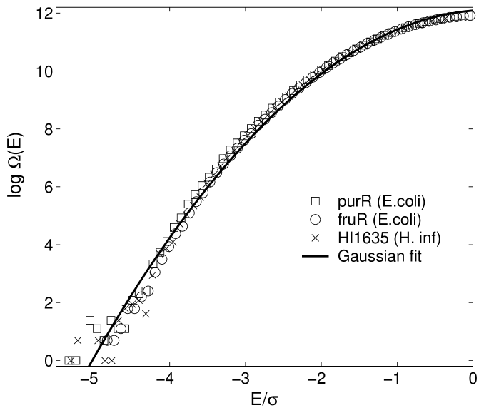
Figure 1: Spectrum of binding energy for three different transcription factors and the Gaussian approximation (solid line).

II.3 Diffusion in a sequence-dependent energy landscape

The whole DNA molecule can thus be mapped onto one-dimensional array of sites $\left\{\vec{s}_{i}\right\}$, each corresponding to a certain binding sequence comprising bases from the $i$-th to the $(i+l-1)$-th, $l$ being the length of the motif (see Fig. 2). At each site, there is a probability $p_{i}$ of hopping to site ${i+1}$ and a probability $q_{i}$ of hopping to site ${i-1}$. These probabilities depend on the specific binding energies $U_{i}$ and $U_{i\pm 1}$ at the $i$-th site and at the adjacent sites respectively and are proportional to the corresponding transition rates, $\omega_{i,i+1}$ and $\omega_{i,i-1}$. For the latter, it is most natural to assume the regular activated transport form

$$\omega_{i,i\pm 1}=\nu\times\left\{\begin{array}[]{l}e^{-\beta\left(U_{i\pm 1}-U_{i}\right)}\qquad{\rm if}~{}U_{i\pm 1}>U_{i}\\ 1.0\qquad\qquad{\rm otherwise}\end{array}\right.,$$ (7)

where $\nu$ is the effective attempt frequency, $\beta\equiv\left(k_{B}T\right)^{-1}$, $k_{B}$ is the Boltzmann constant and $T$ is the ambient temperature. Having defined that, we have a one-dimensional random walk with position-dependent hopping probabilities.

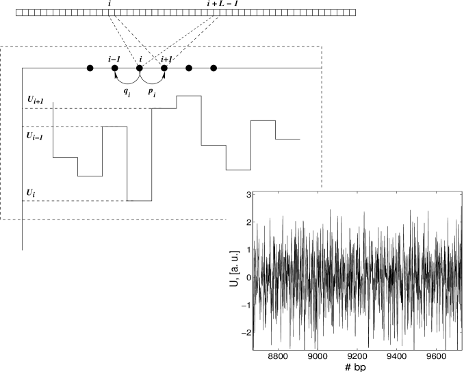
Figure 2: The Model Potential.

As has been shown in numerous papers throughout the last two decades, the properties of 1D random walks can vary dramatically depending on the actual choice of probabilities $\left\{p_{i}\right\}$ (for review, see e. g. Bouchaud and Georges (1990)). Here we employ the mean first-passage time formalism Murthy and Kehr (1989) to derive the diffusion law $\tau_{1d}\left(\bar{n}\right)$ for protein sliding along the DNA given the sequence-dependent binding energy (7).

III Results

Using the model described above, we studied the following problems:

• How fast is the 1D search on DNA as a function of the “roughness” $\sigma$ of the binding energy landscape?

• How significant is the role of non-specific binding energy $E_{\rm ns}$ in determining the search time?

• How fast is the search for the native site under conditions that provide stability to the protein-DNA complex at the target site?

Diffusion along the DNA

We state here the main results without a derivation (which can be found in the Appendix A). For a given set of probabilities $\left\{p_{i}\right\}$, the mean first-passage time (MFPT) from $i=0$ to $i=L$ (in terms of number of steps) is Murthy and Kehr (1989)

$$\bar{t}_{0,L}=L+\sum_{k=0}^{L-1}\alpha_{k}+\sum_{k=0}^{L-2}\sum_{i=k+1}^{L-1}\left(1+\alpha_{k}\right)\prod_{j=k+1}^{i}\alpha_{j},$$ (8)

where $\alpha_{i}\equiv q_{i}/p_{i}$. The relation (8) gives the MFPT for one given realization of probabilities. Assuming that the specific binding energies $\left\{U_{i}\right\}$ have a normal distribution with variance $\sigma^{2}$ (see above), we plug the probabilities in (7) into (8) and after a somewhat lengthy but straightforward calculation, we obtain an expression for the MFPT averaged over genomic sequences for $L\gg 1$:

$$\left\langle\bar{t}_{FP}\left(L\right)\right\rangle\simeq\tau_{0}L^{2}e^{7\beta^{2}\sigma^{2}/4}\left(1+\beta^{2}\sigma^{2}/2\right)^{-1/2},$$ (9)

where $\tau_{0}$ is the reciprocal of the effective attempt frequency for hopping to a neighboring site.

The main result is that the 1D search by hopping to neighboring sites proceeds by normal diffusion with $t\sim L^{2}/2D_{1d}$, where the diffusion coefficient

$$D_{1d}\left(\sigma\right)\simeq\frac{1}{2\tau_{0}}\left(1+\frac{\beta^{2}\sigma^{2}}{2}\right)^{1/2}e^{-7\beta^{2}\sigma^{2}/4}$$ (10)

exhibits an exponential dependence on the “roughness” of the binding energy landscape $\sigma$, dropping rapidly as $\sigma$ becomes greater than few $k_{B}T$ Slutsky et al. (2004). Hence, rapid diffusion of a protein along the DNA is possible only if the roughness of the binding energy landscape is small compared to $k_{B}T$ ($\beta\sigma<1.5$). This requirement imposes strong constraints on the allowed energy of specific binding interactions.

III.1 Optimal time of 3D/1D search

When 1D scanning is combined with 3D diffusion, what is the optimal time a protein has to spend in each of the two regimes? To answer this question we compute the optimal number of sites the protein has to scan by 1D diffusion in order to get the fastest overall search. Results of this section are rather general and are not limited to the particular scenario of slow 1D diffusion on a rough landscape discussed above.

Each time the protein binds DNA it performs a round of 1D diffusion. If the round lasts $\tau_{1d}$ then on average the protein scans $\bar{n}=\sqrt{16D_{1d}\tau_{1d}/\pi}$ bps. Hughes (1995) By plugging this relation into Eq. (3) for search time $t_{s}$, and minimizing $t_{s}$ with respect to $\bar{n}$, we get the optimal total search time and the optimal number of sites to be scanned in each round:

$$t_{s}^{\rm opt}=t_{s}(\bar{n}_{\rm opt})=\frac{M}{2}\sqrt{\frac{\pi\bar{\tau}_{3d}}{D_{1d}}}\ \ \ \ \bar{n}_{\rm opt}=\sqrt{\frac{16}{\pi}D_{1d}\bar{\tau}_{3d}}$$ (11)

This analysis brings us to the following conclusions.

First, and most importantly, we obtain that in the optimal regime of search

$$\tau_{1d}(\bar{n}_{\rm opt})=\tau_{3d},$$ (12)

i.e. the protein spends equal amounts of time diffusing along non-specific DNA and diffusing in the solution. This striking result is very general, and is true irrespective of the values of diffusion coefficients $D_{1d}$ or $D_{3d}$, or size of the genome $M$. In fact it follows directly from the diffusion law $\bar{n}\sim\sqrt{\tau_{1d}}$. More importantly this central result can be verified experimentally by either single-molecule techniques or by traditional methods.

Also note that the optimal region of the DNA scanned in a single round of 1D diffusion $\bar{n}_{\rm opt}$ does not depend on M, i.e. is the same irrespective of the size of the genomes to be searched for a specific site.

Second, the optimal 1D/3D combination reached at $\tau_{1d}=\tau_{3d}$ leads to a significant speed up of the search process. In fact, an optimal 1D/3D search is $\bar{n}_{\rm opt}$ times faster than a search by 3D diffusion alone, and ${M}/{\bar{n}_{\rm opt}}$ times faster than a search by 1D diffusion alone. For example, if the protein operates in the optimal 1D/3D regime and scans $\bar{n}_{\rm opt}=100$bp during each round of DNA binding, then the experimentally measured rate of binding to the specific site can be $100$ times greater than the rate achievable by 3D diffusion alone.

Third, we can estimate $\bar{n}_{opt}$, the maximal number of sites a protein can scan in each round of 1D search. If we set $D_{1d}$ to its maximum, i. e. $D_{1d}\sim D_{3d}$ and $\bar{\tau}_{3d}\sim l_{\rm d}^{2}/D_{3d}$, with $l_{\rm m}\sim 0.1\mu{\rm m}$, we get

$$\bar{n}_{\rm opt}^{\rm max}\sim 500~{}{\rm bp}.$$ (13)

For a smaller 1D diffusion coefficient, e. g. $D_{1d}\sim D_{3d}/100$, we get $\bar{n}_{\rm opt}^{\rm max}\sim 50$bp. Again, single molecule experiments can provide estimates of these quantities for different conditions of diffusion.

Finally, we obtain estimates of the shortest possible total search time. If $M\approx 10^{6}$ bp and 1D diffusion is at its fastest rate, i. e. $D_{1d}\sim D_{3d}=10^{-7}$cm${{}^{2}}/$s, then using Eq. (11) we get

$$t^{opt}_{s}\sim\frac{M}{2}\sqrt{2\pi\bar{\tau}_{3d}\tau_{0}}\sim 5~{}{\rm sec},$$ (14)

where we estimate $\tau_{0}\sim a_{0}^{2}/D_{3d}\sim 10^{-8}$ sec.

One can also estimate the search time using in vitro experimentally measured binding rates in water $k^{\rm water}_{on}\approx 10^{10}$M^-1s^-1 Riggs et al. (1970b, a). The diffusion coefficient of a protein in the cytoplasm is $10-100$ times lower than that in water leading to the estimated binding rate of $k^{\rm cytoplasm}_{on}\approx 10^{8}-10^{9}$M^-1s^-1 (see Appendix D). From this we obtain the time it takes for one protein to bind one site in a cell of $1\mu{\rm m}^{3}$ volume (i.e. [TF]$\approx 10^{-9}$M) as

$$t^{exp}_{s}={\left(k^{\rm cytoplasm}_{on}{\rm[TF]}\right)^{-1}}\sim 1-10~{}{\rm sec}.$$ (15)

One can see perfect agreement between our theoretical estimates and experimentally measured binding rates.

As we mentioned above, there are usually several TF molecules searching in parallel for the target site. Naturally, in this case, the search is sped up proportionally to the number of molecules.

III.2 Diffusion of PurR on E.coli genome

To check the applicability of the above considerations, we simulated one - dimensional diffusion of $PurR$ transcription factor on the $E.~{}coli$ chromosome.

The specific energy profile was built using a weight matrix derived from 35 $PurR$ binding sites following a standard procedure described elsewhere Berg and von Hippel (1987), Stormo and Fields (1998). The resulting energy profile is random and uncorrelated and has a standard deviation $\sigma\simeq 6.5~{}k_{B}T$. This profile was used as an input for calculating mean first passage time at different temperatures. The result of these calculations is presented in Fig. 3. It is clear that when the roughness of the landscape becomes significant $\sigma>2k_{B}T$, the diffusion proceeds extremely slowly. Only $\sim 10-100$ bp can be scanned by a TF when $\sigma=2k_{B}T$. A natural requirement for sufficiently fast diffusion is, as before, $\sigma\sim k_{B}T$.

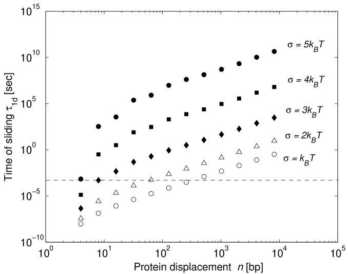
Figure 3: The mean first passage time vs traveling distance for $purR$ transcription factor on the binding landscapes of different roughness (or at different temperatures). The horizontal line indicates the optimal regime, $\tau_{1d}\sim\bar{\tau}_{3d}$.

III.3 Non-specific binding

While the diffusion of the TF molecules along DNA is controlled by the specific binding energy, the dissociation of the TF from the DNA depends on the total binding energy, i. e. on the non-specific binding as well as on the specific one. Moreover, since the dissociation events are much less frequent than the hopping between neighboring base-pairs (roughly by a factor of $\bar{\tau}_{3d}/\left\langle\tau\right\rangle$), the non-specific energy $E_{\rm ns}$ makes a sensibly larger contribution to the total binding energy.

For a TF at rest bound to some DNA site $i$, the dissociation rate $r_{i}$ would be given by the Arrhenius - type relation,

$$r_{i}=\frac{1}{\tau_{0}}e^{-\beta\left(E_{\rm ns}-U_{i}\right)}.$$ (16)

Given the specific $U_{i}$ non-specific $E_{\rm ns}$ energy one can calculate the average time $\tau_{1d}$ a protein spends before dissociating from the DNA (see Appendix B). We obtain

$$E_{\rm ns}=k_{B}T\left[\ln\left(\frac{\tau_{1d}}{\tau_{0}}\right)-\frac{1}{2}\left(\frac{\sigma}{k_{B}T}\right)^{2}\right],$$ (17)

and in the optimal regime where $\tau_{1d}=\bar{\tau}_{3d}$

$$E^{\rm opt}_{\rm ns}=k_{B}T\left[\ln\left(\frac{\tau_{3d}}{\tau_{0}}\right)-\frac{1}{2}\left(\frac{\sigma}{k_{B}T}\right)^{2}\right].$$ (18)

III.4 The parameter space

Since for a given value of $\sigma$, the non-specific binding controls the dissociation rate, the search time will deviate from the optimum if $E_{\rm ns}$ moves from this predetermined value. In Fig. 4a we plot the search time as a function of the non-specific binding energy for different values of $\sigma$.

We now define the tolerance factor $\zeta$ as the ratio between the acceptable value of the search time $t_{s}$ and the optimal search time $t^{\rm opt}_{s}$. Experimental data suggest $\zeta\leq 5$, but for the moment we allow for much larger values of $\zeta\sim 10-100$ (this can be done when, for instance, there are many protein molecules searching in parallel). As we can see from Fig. 4a, for each value of $\sigma$, there is a range of possible values of $E_{\rm ns}$ such that the resulting search time is within the region of tolerance (see Appendix B). Notice the dramatic increase in the search time as $E_{\rm ns}$ deviates from its optimal value.

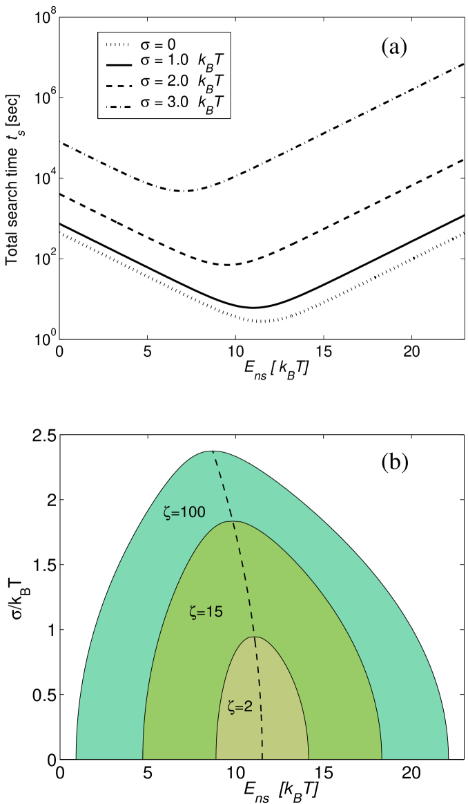
Figure 4: (a) Dependence of the search time on the non-specific binding energy. (b) The parameter space. The dashed line corresponds to optimal parameters $\sigma$ and $E_{ns}$ connected by Eq. (18).

Specifying $\zeta$, we can define our parameter space, i. e. the values of specific and non-specific energy producing a total search time within the region of tolerance. In Fig. 4b, we consider three values of $\zeta$. The most relaxed requirement $\zeta=100$ provides a search time $t_{s}\leq 500~{}{\rm sec}$. If $100$ proteins are searching for a single site, then the first one will find it after $\sim 5~{}{\rm sec}$, leading however to a fairly low binding rate of $k_{\rm on}\approx 1/500~{}\rm{sec}\cdot 10^{9}~{}{\rm M}^{-1}=2\cdot 10^{6}~{}{\rm M}^{-1}{\rm s}^{-1}$ (compared to experimentally measured $10^{10}~{}{\rm M}^{-1}{\rm s}^{-1}$ in water). Importantly, in order to comply with even this most relaxed search time requirement, the characteristic strength of specific interaction must be smaller than $\sim 2.3~{}k_{B}T$.

These results bring us to a very important conclusion that a protein cannot find its site in biologically relevant time if the roughness of the specific binding landscape is greater than $\sim 2~{}k_{B}T$. Although an optimal 1D/3D combination can speed up the search, it cannot overcome the slowdown of 1D diffusion. Only fairly smooth landscapes ($\sigma\sim 1k_{B}T$) can be effectively navigated by proteins.

IV Speed versus stability

While rapid search requires fairly smooth landscapes ($\sigma\sim 1k_{B}T$), stability of the protein-DNA complex, in turn, requires a low energy of the target site ($U_{min}<15~{}k_{B}T$ for a genome of $10^{6}$ bp).

In Fig. 5a, we present the equilibrium probability $P_{b}$ of binding the strongest target site with energy $U_{\rm min}=U_{0}$ Gerland et al. (2002) as a function of $\sigma/k_{B}T$. In equilibrium, $P_{b}$ equals the fraction of time the protein spends at the target site:

$$P_{b}=\frac{\exp\left[-\beta U_{\rm 0}\right]}{\sum_{i=0}^{M}\exp\left[-\beta U_{i}\right]}.$$ (19)

Since the target site is not separated from the rest of the distribution by a significant energy gap, $P_{b}$ is comparable to 1 (which is the natural requirement for a good regulatory site) only at $\sigma$ much greater than $k_{B}T$.

Figure 5b shows the optimal search time at the corresponding values of $\sigma/k_{B}T$. High roughness of $\sigma>>k_{B}T$ required for stability of the protein-DNA complex leads to astronomically large search times. In contrast, a protein can effectively search the target site at $\sigma$ smaller than $1-2k_{B}T$.

This brings us to the central result that the ability to translocate rapidly along the DNA clearly cannot comply with the stability requirement.

Requirement of high stability at the target site $P_{b}\sim 1$ (or $P_{b}\sim 1/N_{p}$ if $N_{p}$ copies of the protein are present) yields an estimate for the minimal $\sigma$,

$$\sigma\sim k_{B}T\sqrt{2\ln M}\simeq 5~{}k_{B}T,$$ (20)

given a genome size $M=10^{6}$.

From the above analysis, an obvious conflict arises: the same energy landscape cannot allow for both rapid translocation and high stability of states formed at sites with the lowest energy. This conflict is similar to the speed-stability paradox of protein folding formulated by Gutin $et.al.$ Gutin et al. (1998): rapid search in conformation space requires a smooth energy landscape, but then the native state is unstable. In protein folding, this conflict is resolved by the presence of a large energy gap between the native state and the rest of the conformations Finkelstein and Ptitsyn (2002); Pande et al. (2000).

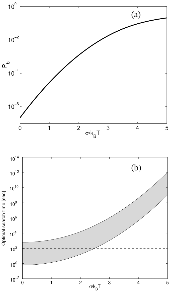
Figure 5: (a) Stability on the protein-DNA complex on the cognate site measured as the fraction of time in the bound state at equilibrium. (b) Optimal search time as a function of the binding profile roughness, for the range of parameters $10^{-4}{\rm sec}\leq\tau_{3d}\leq 10^{-2}{\rm sec}$, $10^{-10}{\rm sec}\leq\tau_{0}\leq 10^{-6}{\rm sec}$.

As evident from Fig. 1, no such energy gap separates cognate sites from the bulk of other (random) sites. In fact, the energy function in the form of (5) cannot, in principle, provide a significant energy gap. Increasing the number of TFs cannot resolve the paradox either (see Appendix D,E). An alternative solution must be sought.

V The two-mode model

The “search speed - stability” paradox has already been qualitatively anticipated by Winter, Berg and von Hippel Winter et al. (1989), who therefore concluded that a conformational change of some sort should exist that would allow fast switching between “specific” and “non-specific” modes of binding. In the non-specific mode, the protein is “sliding” over an essentially equipotential surface (in our terms, $\sigma_{\rm non-spec}=0$) whereas site-binding takes place in the “specific” mode ($\sigma_{\rm spec}\gg k_{B}T$). A protein in the non-specific binding mode is “unaware” of the DNA sequence it is bound to. Thus, it should permanently alternate between the binding modes, probing the underlying sites for specificity.

This model naturally rises a question about the nature of the conformation change. Originally, it was described as a “microscopic” binding of the protein to the DNA accompanied by water and ion extrusion. However, numerous calorimetry measurements and calculations Spolar and Record (1994) show that such a transition is usually accompanied by a large heat capacity change $\Delta C$. This $\Delta C$ cannot be accounted for, unless additional degrees of freedom, namely, protein folding, are taken into account. On-site folding of the transcription factor may involve significant structural change Flyvbjerg et al. (2002); Bruinsma (2002); Kalodimos et al. (2004) and take a time of $\sim 10^{-4}..10^{-6}~{}$sec Akke (2002) (compared to a characteristic on-site time of $\tau_{0}\sim 10^{-7}..10^{-8}~{}$sec). We conclude that conformational transition between the two modes involves (but not limited to) partial folding of the TF.

If the TF is to probe every site for specificity in this fashion, it would take hours to locate the native site. We note, however, that if there was a way to probe only a very limited set of sites, i. e. only those having high potential for specificity, the search time would be dramatically reduced. From the previous section it is clear that a relatively weak site-specific interaction (i.e. smooth landscape, $\sigma\sim k_{B}T$) does not affect significantly the diffusive properties of the DNA and the total search time. If this landscape, however, is correlated with the actual specific binding energy landscape (with $\sigma\sim 5-6~{}k_{B}T$), the specific sites will be the strongest ones in both modes. The protein conformational changes should occur therefore mainly at these sites, which constitute “traps” in the smooth landscape. Since such sites constitute a very small fraction of the total number of sites, the transitions between the modes are very rare.

We therefore suggest that there are two modes of protein-DNA binding: the search mode and the recognition mode (Fig. 6). In the search mode, the protein conformation is such that it allows only a relatively weak site-specific interaction ($\sigma_{\rm s}\sim 1.0-2.0~{}k_{B}T$) (Fig 6 top). In the recognition mode, the protein is in its final conformation and interacts very strongly ($\sigma_{\rm r}\geq 5~{}k_{B}T$) with the DNA (Fig 6 bottom). If two energy profiles are strongly correlated then the lowest lying energy levels (“traps”) in the search mode ($\leq-5~{}k_{B}T$) are likely to correspond to the strongest sites in the recognition mode, putatively, the cognate sites. The transitions between the two modes happen mainly when the protein is trapped at a low-energy site of the search landscape. In this fashion, the 1D diffusion coefficient $D_{1d}$ is about 10–100 times smaller than the ideal limit, but the search time in the optimal regime is reduced only by a factor of $\sim 3-10$ (see Eq. (11)).

The coupling between the conformational change and association at a site with a low-energy trap is likely to take place through time conditioning. Namely, the folding (or a similar conformation transition) occurs only if the protein spends some minimal amount of time bound to a certain site. This statement is basically equivalent to saying that the free energy barrier that the protein must overcome to transform to the final state must be comparable to the characteristic energy difference that controls hopping to the neighboring sites.

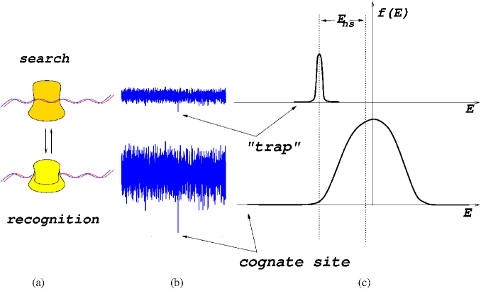
Figure 6: Cartoon demonstrating the two-mode search-and-fold mechanism. Top: search mode, bottom: recognition mode (a) two conformations of the protein bound to DNA: partially unfolded (top) and fully folded (bottom). (b) The binding energy landscape experienced by the protein in the corresponding conformations. (c) The spectrum of the binding energy determining stability of the protein in the corresponding conformations.

The protein conformation in recognition mode should be stabilized by additional protein-DNA interactions. If these interactions are unfavorable, the folded structure is destabilized, then the search conformation is rapidly restored and the diffusion proceeds as before. If the new interactions are favorable, the folded structure is stable and the protein is trapped at the site for a very long time.

For this mechanism to work, transition between the two modes of search has to be associated with significant change in the free energy ($\sim 5..10k_{B}T$) of the protein-DNA complex (see Fig 6(c)). Such energy difference between the two states is required to make most of the high-energy sites in the recognition mode less favorable than in the search mode. So a protein would rather (partially) unfold that bind an unfavorable site. As a result sites that lay higher in energy than a certain cutoff exhibit similar non-specific binding energy (i.e. switch into search mode of binding). Folding of partially disorder protein loops or helices can provide required free energy difference between the two modes.

Efficiency of proposed search-and-fold mechanism depends on the energy difference between the two modes, correlation between the energy profiles and the barrier between the two states. The barrier determines the rate of partial folding-unfolding transition. If the barrier is too low, then the protein equilibrates while on a single site having no effect on search kinetics. On the contrary, too high barrier can lead to rear folding events and the cognate site can be missed. It can be shown that proper size of the barrier provides efficient search and stable protein-DNA complex. Alternatively, the cognate site can lower the barrier by stabilizing the transition state (i.e. the folding nucleus Abkevich et al. (1994); Mirny and Shakhnovich (2001)) acting as a catalyst of partial folding. Quantitative analysis of these factors is beyond the scope of this study and will be published elsewhere.

VI Discussion

VI.1 Specificity “for free”: kinetics vs thermodynamics.

The proposed mechanism of specific site location is akin to kinetic proofreading Hopfield (1974), which is a very general concept for a broad class of high-specificity biochemical reactions. The required specificity is achieved in kinetic proofreading through formation of an intermediate metastable complex that paves the way for irreversible enzymatic reaction. If the reaction is much slower than the life-time of the complex, then substrates that spend enough time in the complex are subject to the enzymatic reaction, while substrates that form short-lived complexes are released back to the solvent before the reaction takes place. In other words, the substrates are selected by kinetic partitioning.

In contrast to kinetic proofreading that increases equilibrium specificity for the price of energy consumption, the search-and-fold model doesn’t require any additional source of energy. The two mode search-and-fold model provides faster “on-rate” of binding while keeping the equilibrium binding constant unchanged. Naturally, the “off-rate” is increased as well. This makes our two-mode model thermodynamically “neutral”.

VI.2 Coupling of folding and binding in molecular recognition

Several DNA- and ligand-binding proteins are known to have partially unfolded (disordered) structures in the unbound state. The unstructured regions fold upon binding to the target. Does binding-induced folding provide any biological advantage?

The idea of coupling between local folding and site binding has been around for some time and was recently reassessed in the much broader context of intrinsically unstructured proteins Wright and Dyson (1999); Dyson and Wright (2002); Uversky (2002). Induced folding of these proteins can have several biological advantages. First, flexible unstructured domains have intrinsic plasticity allowing them to accommodate targets/ligands of various size and shape. Second, free energy of binding is required for compensation for entropic cost of ordering of the unstructured region. A poor ligand that doesn’t provide enough binding free energy cannot induce folding and, hence, can not form a stable complex. Williams et.al. have suggested that unstructured domains can be result of evolutionary selection that acts on the bound (structured) conformation, while ignoring the unbound (unstructured) conformation Williams et al. (2001). Partial unfolding can also increase protein’s radius of gyration and, hence, increase the binding rate Shoemaker et al. (2000); Levy et al. (2004)

Here we propose a mechanism that suggests role of induced folding in providing rapid and specific binding. Induced folding (or other sort of two-state conformational transition) allows a protein to search and recognize DNA in two different conformations providing rapid binding to the target site. Importantly, this mechanism reconciles rapid search for the target site with stable bound complex (see above). The rate of induced folding can also play a role in determining the specificity of recognition (Slutsky and Mirny, in preparation).

Structural and thermodynamic data argue in favor of distinct protein conformations for search along non-cognate DNA and for recognition of the target site. Proteins such as $\lambda$ cI, Eco RV and GCN4 apparently do not fold their unstructured regions while bound to non-cognate DNA Winkler et al. (1993); Clarke et al. (1991); O’Neil et al. (1990), supporting our hypothesis.

Heat capacity measurements on a vast variety of protein-DNA complexes report a large negative heat capacity change in site-specific recognition, which is a clear indication of a phase transition. These measurements supplemented by X-ray crystallography and NMR structural data were interpreted by Spolar $et.~{}al.$ Spolar and Record (1994) mainly in terms of hydrophobic and conformational contributions to entropy. Thus, folding - binding coupling is now considered a well established effect for a large set of transcription factors.

However, real-time kinetic measurements were not performed until recently, so that the question of the actual mechanism was left open. Serious advances in this direction were made by Kalodimos $et.~{}al.$ Kalodimos et al. (2001, 2002, 2004), who observed a two-step site recognition by dimeric $Lac$ repressor. The H/D-exchange NMR data unambiguously demonstrates site pre-selection by $\alpha$-helices bound in the major groove followed by folding of hinge helices that bind to the minor groove elements and complete the specific site recognition. Though the experiments in this field were performed with a single model system, their implications are likely to have a general character.

It should be mentioned, that no transition of this kind is observed when the protein is unbound from DNA. A possible reason for this can be a significant reduction of the free energy barrier for folding, entropic in essence, that accompanies protein-DNA association. Entropy barrier reduction is a natural consequence of relative anchoring of the various parts of the protein on the DNA “scaffold”. Thermal fluctuations that the associated protein is subject to are generally of the order of $\sim k_{B}T$, and their main effect is protein translocation along the DNA. From the above analysis, it follows that the translocation actually takes place only if the protein encounters barriers of $\sigma_{\rm s}\sim k_{B}T$ on its way. In a large enough collection of sites ($M\gg 1$), however, potential “wells” of depth $\sim\sigma_{\rm s}\sqrt{2\ln M}$ will be present. If the “well” depth is larger than the folding barrier height, the probability of on-site (“in-well”) folding increases, leading eventually to a stable complex formation. More detailed computational analysis of coupling between folding and binding will be published elsewhere.

VI.3 Biological implications

Mechanism of 3D/1D search described above has several biological implications. Needless to say that studied model (as any quantitative model) is a gross simplification of protein-DNA recognition in vivo. In spite of this simplification, proposed mechanism can be generalized to describe in vivo binding. Here we briefly discuss some biological implications of our model.

VI.3.1 Simultaneous search by several proteins

If several TFs are searching for its site on the DNA, the total search time is given by equation (15) and is obviously shorter than the time for a single TF. For example, if $100$ copies of a TF are searching in parallel for the cognate site, then assuming $k^{\rm cytoplasm}_{on}\approx 10^{8}$M^-1s^-1 and a cell of $1\mu{\rm m}^{3}$ volume, we obtain the search time of $t_{s}\approx 0.1{\rm sec}$. Increasing the number of TF molecules can further decrease the search time, but can have harmful effects due to molecular crowding in the cell. Note, however, that increasing the number of TF molecules to $100-1000$ per cell cannot resolve the speed-stability paradox (see Fig. 5).

VI.3.2 Search inside a cell: molecular crowding on DNA and chromatin

Above we assumed that a TF is free to slide along the DNA. In vivo picture is complicated by other proteins and protein complexes (nucleosomes, polymerases etc) bound to DNA, preventing a TF to slide freely along DNA. What are the effects of such molecular crowding on the search time?

Our model suggests that molecular crowding on DNA can have little effect on the search time if certain conditions are satisfied. Obviously, the the cognate shall not be screened by other DNA-bound molecules/nucleosomes. DNA-bound molecules can interfere with the search process by shortening regions of DNA scanned on each round of 1D diffusion. If, however, the distance between DNA-bound molecules/nucleosomes in the vicinity of the cognate site is greater than $\bar{n}_{\rm opt}\sim 300-500~{}{\rm bp}$ (eq. (13) and Kim et al. (1987)), then obstacles on the DNA do not shorten the rounds of 1D diffusion and, hence, do not slow down the search process. Our analysis also suggests that sequestration of part of genomic DNA by nucleosomes can even speed up the search process.

If DNA-bound proteins are separated by more than $300-500$bp E.coli genomic DNA can accommodate $4.6\times 10^{6}{\rm bp}/300{\rm bp}\approx 1.5\times 10^{4}$ proteins. In other words all $150$ known and predicted E.coli TF can be simultaneously present in $100$ copies of each and search for their cognate sites without affecting each other. (In fact they can be present in $200$ copies each since optimal search requires $50\%$ of proteins to be in solution at any time). On the other hand, a short $\sim 50{\rm bp}$ linker between nucleosomes in eukaryotic chromatin can increase the search time about $10$-fold. Details of this analysis will be published elsewhere.

VI.3.3 “Funnels”, local organization of sites

Several known bacterial and eukaryotic sites tend to cluster together. One may suggest that such clustering or other local arrangement of sites can create a “funnel” in the binding energy landscape leading to a more rapid binding of cognate sites. Our model suggests that even if such “funnels” do exist, they would not significantly speed up the search process. Proposed search mechanism involves $\sim M/\bar{n}_{\rm opt}\sim 10^{4}$ rounds of 1D/3D diffusions. So a TF spends all the search time far from the cognate site. Only the last round (out of $10^{4}$) will be sped up by the “funnel”, leading to no significant decrease of the search time.

Local organization of sites and other sequence-dependent properties of the DNA structure (flexibility of AT-rich regions, DNA curvature on poly-A tracks etc) may influence preferred localization of TFs and lead to faster on-/off- binding rates and fast equilibration on neighboring sites (see Slutsky et al. (2004) for details).

VI.3.4 Protein hopping: intersegment transfer

Our model assumed that rounds of 1D diffusion are separated by periods of 3D diffusion. Intersegment transfer is another mechanism that can be involved. If two segments of DNA come close to each other, a TF sliding along one segment can “hop” to another. The benefit of this mechanism is that it significantly shortens the transfer time $\tau_{3D}$. Several experimental evidences suggest that tetrameric LacI, which has two DNA-binding sites, travels along DNA through 1D diffusion and intersegment transfer.

We did not consider this mechanism because of the two following considerations. First, it is unclear whether TFs that have only one binding site can perform intersegment transfer. Second, for this mechanism to work, distant segments of DNA need to come close to each other. While DNA packed into a cell/nuclear volume crosses itself every $\sim 500$bp, DNA in solution (at in vitro concentrations) is unlikely to have any such self-crossings. Hence intersegment transfer cannot explain “faster than diffusion” binding rates observed in vitro. This mechanism however may play a role in vivo, especially for proteins that have multiple DNA-binding sites.

VI.4 Proposed experiments

Our results propose several experimentally testable predictions.

First, we predict that the maximal rate of binding is achieved when the protein spends half of the time in solution and half sliding along the DNA. This result can be readily verified experimentally by measuring concentration of free protein in solution that contains DNA but no cognate site. We also show how the search time depends on the energy of non-specific binding, that, in turn, can be controlled by ionic strength of solution or by engineering proteins with stronger or weaker non-specific binding. In vivo observation of the ”50/50” rule would suggest that proteins are optimized by evolution for rapid search.

Second, we show how binding rate depends on the average travel time between two random segments of DNA, $\tau_{3d}$. Time $\tau_{3d}$ depends on the DNA concentration and domain organization of DNA. By changing DNA concentration and/or DNA stretching in a single molecule experiment one can alter $\tau_{3d}$ and thus study the role of DNA packing on the rate of binding. This effect has implications for DNA recognition in vivo, where DNA is organized and domains. Similarly one can experimentally measure and compare with analytical predictions the binding rate in the presence of other DNA-binding proteins or nucleosomes.

Single molecule experiments and AFM/SFM imaging allow direct observation of protein trajectory and measurement of the 1D diffusion coefficient, $D_{1d}$ on non-cognate DNA. Our formalism, in turn, allows to calculate the spectrum of specific binding energy given $D_{1d}$. Such measurements can be direct tests of our conjecture that 1D search along non-cognate DNA proceeds along a “smoother” energy profile.

Third, using protein engineering one can stabilize unstructured regions of DNA-binding proteins (e.g. $\lambda$ cI, Eco RV and GCN4) and study binding rates of these engineered rigid protein. Such experiments can test proposed search-and-fold mechanism and shed light on the role of unstructured regions in determining stability, specificity and binding rates.

We also suggest that proteins bound to non-cognate DNA are not fully ordered. Unfortunately very few studies Kalodimos et al. (2001, 2002, 2004) have addressed the mechanisms of binding to non-cognate DNA. More studies of structures, thermodynamics and dynamics of proteins bound to non-cognate DNA will deepen our understanding of specific protein-DNA recognition.

VII Conclusions

We have developed a quantitative model of protein-DNA interaction that provides an insight into the mechanism of fast target site location. We found the range of parameters (specific and non-specific binding energies) that are crucial for fast search and, hence, robust functioning of gene transcription. Paradoxically, realistic energy cannot provide both rapid search and strong binding of a rigid protein. This allowed us to formulate speed-stability paradox of protein-DNA recognition (which is similar to famous Levinthal paradox of protein folding). To resolve this paradox we proposed a search-and-fold mechanism that involves the coupling of protein binding and protein folding.

Proposed mechanism has several important biological implications explaining how a protein can find its site on DNA in vivo in the presence of other proteins and nucleosomes, and by simultaneous search of several proteins. Our model provides, for the first time, quantitative framework for analysis of kinetics of transcription factor binding and, hence, gene expression. Importantly, our model links molecular properties of transcription factors to the timing of transcription activation. Proper understanding of the entire mechanism will hardly be possible without further experimental effort in these directions.

Appendix A: Diffusive properties of the DNA.

The derivation consists of two steps. First, we describe the random walk along the DNA in terms of number of steps. Next, we calculate the mean time between successive steps in a random energetic landscape which provides the time - scale for the problem. Such a decoupling, strictly speaking, does not hold when the number of steps is small, i. e. when the number of visited sites is small and the random quantities are not averaged properly. However, since we are dealing with large numbers of steps ($\sim 10^{5}-10^{6}$) this approach is legal, which is also confirmed by numerical simulations.

The MFPT.

To derive the diffusion law, we calculate the mean first passage time (MFPT) from site $\#0$ to site $\#L$, defined as the mean number of steps the particle is to make in order to reach the site $\#L$ for the first time. The derivation here follows the one in Murthy and Kehr (1989).

Let $P_{i,j}\left(n\right)$ denote the probability to start at site $\#i$ and reach the site $\#j$ in exactly $n$ steps. Then, for example,

$$P_{i,i+1}\left(n\right)=p_{i}T_{i}\left(n-1\right),$$ (21)

where $T_{i}\left(n\right)$ is defined as the probability of returning to the $i$-th site after $n$ steps without stepping to the right of it. Now, all the paths contributing to $T_{i}\left(n-1\right)$ should start with the step to the left and then reach the site $\#i$ in $n-2$ steps, not necessarily for the first time. Thus, the probability $T_{i}\left(n-1\right)$ can be written as

$$T_{i}\left(n-1\right)=q_{i}\sum_{m,l}P_{i-1,i}\left(m\right)T_{i}\left(l\right)\delta_{m+l,n-2}.$$ (22)

We now introduce generating functions

$$\tilde{P}_{i,j}\left(z\right)=\sum_{n=0}^{\infty}z^{n}~{}P_{i,j}\left(n\right),\qquad\tilde{T}_{i}\left(z\right)=\sum_{n=0}^{\infty}z^{n}~{}T_{i}\left(n\right).$$ (23)

One can easily show (see e. g. Goldhirsh and Gefen (1986)) that

$$\tilde{P}_{0,L}\left(z\right)=\prod_{i=0}^{L-1}\tilde{P}_{i,i+1}\left(z\right).$$ (24)

Knowing $\tilde{P}_{i,i+1}\left(z\right)$, one calculates the MFPT straightforwardly as

$$\bar{t}_{0,L}=\frac{\sum_{n}nP_{0,L}\left(n\right)}{\sum_{n}P_{0,L}\left(n\right)}=\left[\frac{d}{dz}\ln\tilde{P}_{0,L}\left(z\right)\right]_{z=1}$$

$$=\sum_{i=0}^{L-1}\left[\frac{d}{dz}\ln\tilde{P}_{i,i+1}\left(z\right)\right]_{z=1}.$$ (25)

Using (21) and (22), we obtain the following recursion relation for $\tilde{P}_{i,i+1}\left(z\right)$:

$$\tilde{P}_{i,i+1}\left(z\right)=\frac{zp_{i}}{1-zq_{i}\tilde{P}_{i-1,i}\left(z\right)}.$$ (26)

To solve for $\bar{t}_{0,L}$, we must introduce boundary conditions. Let $p_{0}=1,~{}q_{0}=0$, which is equivalent to introducing a reflecting wall at $i=0$. This boundary condition clearly influences the solution for short times and distances. However, as numerical simulations and general considerations suggest, its influence relaxes quite fast, so that for longer times, the result is clearly independent of the boundary. The benefit of setting $p_{0}=1$ becomes clear when we observe that

$$\tilde{P}_{0,1}\left(1\right)=1\qquad\Rightarrow\qquad\forall~{}i\qquad\tilde{P}_{i,i+1}\left(1\right)=1.$$ (27)

Hence,

$$\bar{t}_{0,L}=\sum_{i=0}^{L-1}\tilde{P}_{i,i+1}^{\prime}\left(1\right).$$ (28)

The recursion relation for $P_{i,i+1}^{\prime}\left(1\right)$ is readily obtained from (26) :

$$\tilde{P}_{i,i+1}^{\prime}\left(1\right)=\frac{1}{p_{i}}+\frac{q_{i}}{p_{i}}\tilde{P}_{i-1,i}^{\prime}\left(1\right)=1+\alpha_{i}\left[1+\tilde{P}_{i-1,i}^{\prime}\left(1\right)\right],$$ (29)

with $\alpha_{i}\equiv p_{i}/q_{i}$. Thus, the expression for $\bar{t}_{0,L}$ is obtained in closed form

$$\bar{t}_{0,L}=L+\sum_{k=0}^{L-1}\alpha_{k}+\sum_{k=0}^{L-2}\sum_{i=k+1}^{L-1}\left(1+\alpha_{k}\right)\prod_{j=k+1}^{i}\alpha_{j}.$$ (30)

This solution expression gives MFPT in terms of a given realization of disorder producing a certain set of probabilities $\{p_{i}\}$, whereas we are interested in the behavior averaged over all realizations of disorder. The cumulative products in (30) reduce to the two form $e^{\beta\left(U_{i}-U_{j}\right)}$, which after being averaged over uncorrelated Gaussian disorder produce a factor of $e^{\beta^{2}\sigma^{2}}$. After the summations are carried out, the expression for MFPT becomes for $L\gg 1$

$$\left\langle\bar{t}_{0,L}\right\rangle\simeq L^{2}e^{\beta^{2}\sigma^{2}}.$$ (31)

Thus, the diffusion law appears to be the classical one, with a renormalized diffusion coefficient.

The time constant.

Consider a particle at site $\#i$. The particle will eventually escape to one of the neighboring sites $\#(i\pm 1)$, the escape rate being

$$r_{i}=\omega_{i,i+1}+\omega_{i,i-1}.$$ (32)

To calculate the characteristic diffusion time constant $\langle\tau\rangle$, this rate should be averaged over all configurations of disorder $\{U_{i}\}$. To obtain an analytic expression for the $\langle\tau\rangle$, we assume the form

$$\omega_{i,i\pm 1}=\nu e^{-\beta\left(U_{i\pm 1}-U_{i}\right)}$$ (33)

for both $U_{i\pm 1}>U_{i}$ and $U_{i\pm 1}<U_{i}$ , as opposed to the form (7). Numerics show that this approximation introduces an up to $\sim 15\%$ error for small values of $\beta\sigma$ and is practically exact for $\beta\sigma>2$. Thus,

$$r_{i}=\frac{1}{2\tau_{0}}\left(e^{-\beta\left(U_{i+1}-U_{i}\right)}+e^{-\beta\left(U_{i-1}-U_{i}\right)}\right),$$ (34)

where $\tau_{0}=1/(2\nu)$. The mean time between the successive steps can be calculated therefore as the average over all possible configurations of $U_{i}$, $U_{i\pm 1}$ of the reciprocal of the escape rate, i. e.

$$\left\langle\tau\right\rangle=\left\langle\frac{1}{r_{i}}\right\rangle=2\tau_{0}\int_{-\infty}^{\infty}dU_{i}dU_{i+1}dU_{i-1}\frac{f\left(U_{i}\right)f\left(U_{i+1}\right)f\left(U_{i-1}\right)}{e^{-\beta\left(U_{i+1}-U_{i}\right)}+e^{-\beta\left(U_{i-1}-U_{i}\right)}}.$$ (35)

Assuming as above Gaussian energy statistics, this integral is evaluated as follows

$$\left\langle\tau\right\rangle=\frac{\tau_{0}~{}e^{\beta^{2}\sigma^{2}/2}}{\pi}\int_{-\infty}^{\infty}dxdy\frac{e^{-(x^{2}+y^{2})/2}}{e^{-\beta\sigma x}+e^{-\beta\sigma y}}.$$ (36)

After the change of variables

$$s=\frac{1}{\sqrt{2}}(x+y),\qquad t=\frac{1}{\sqrt{2}}(x-y),$$ (37)

the integral factorizes leading to

$$\left\langle\tau\right\rangle = \frac{\tau_{0}~{}e^{\beta^{2}\sigma^{2}/2}}{2\pi}\int_{-\infty}^{\infty}ds~{}e^{-s^{2}/2+\beta\sigma s/\sqrt{2}}\int_{-\infty}^{\infty}dt\frac{e^{-t^{2}/2}}{\cosh(\beta\sigma t/\sqrt{2})}$$

$$= \frac{\tau_{0}~{}e^{3\beta^{2}\sigma^{2}/4}}{\sqrt{2\pi}}\int_{-\infty}^{\infty}dt~{}e^{-t^{2}/2-\ln\left[\cosh(\beta\sigma t/\sqrt{2})\right]}$$

$$\simeq \frac{\tau_{0}~{}e^{3\beta^{2}\sigma^{2}/4}}{\sqrt{2\pi}}\int_{-\infty}^{\infty}dt~{}e^{-t^{2}(1+\beta^{2}\sigma^{2}/2)/2}={\tau_{0}}~{}e^{3\beta^{2}\sigma^{2}/4}\left[1+\beta^{2}\sigma^{2}/2\right]^{-1/2}$$

Now, multiplying (31) by $\left\langle\tau\right\rangle$, we obtain the diffusion coefficient as

$$D_{1d}\left(\sigma\right)\simeq\frac{1}{2\tau_{0}}\left(1+\frac{\beta^{2}\sigma^{2}}{2}\right)^{1/2}e^{-7\beta^{2}\sigma^{2}/4}.$$ (39)

Appendix B: Non-specific energy

To find how the non-specific energy $E_{\rm ns}$ is related to the average time $\tau_{1d}$ protein spends scanning a single region of the DNA we use simple observation that

$$\left\langle\sum_{i}\tau_{i}r_{i}\right\rangle=1\ \ \ \ \left\langle\sum_{i}\tau_{i}\right\rangle=\tau_{1d}$$ (40)

which states that ”on average” protein dissociates ones from the region it scans.

Since some massive hopping from site to site takes place before the particle eventually dissociates, the dissociation rates and, consequently, the non-specific binding energy should satisfy the following equation

$$\left\langle\sum_{i}\tau_{i}r_{i}\right\rangle=\frac{1}{\tau_{0}}\left\langle\sum_{i}\tau_{i}e^{-\beta\left(E_{\rm ns}-U_{i}\right)}\right\rangle=\frac{1}{\tau_{0}}\int_{-\infty}^{\infty}e^{-\beta\left(E_{\rm ns}-U\right)}\tau\left(U\right)f\left(U\right)dU=1,$$ (41)

and this subject to a condition

$$\left\langle\sum_{i}\tau_{i}\right\rangle=\int_{-\infty}^{\infty}\tau\left(U\right)f\left(U\right)dU=\tau_{1d}.$$ (42)

Where $\tau_{i}$ is the time TF spends at the $i$-th site and $\tau_{1d}$ is the average time of 1D search to dissociation.The average lifetime $\tau_{i}=\tau\left(U_{i}\right)$ at that site is proportional to $\exp\left(-\beta U_{i}\right)$. In this specific case, the particle usually escapes to one of the neighboring sites, and we should average over their energies. Hence, the explicit form $\tau\left(U\right)$ as calculated from (42) is

$$\tau\left(U\right)=\tau_{1d}e^{-\beta^{2}\sigma^{2}/2}e^{-\beta U}.$$ (43)

Substituting this into (41), we have

$$\frac{\tau_{1d}}{\tau_{0}}e^{-\frac{1}{2}\beta^{2}\sigma^{2}-\beta E_{\rm ns}}=1,$$ (44)

or

$$E_{\rm ns}=k_{B}T\left[\ln\left(\frac{\tau_{1d}}{\tau_{0}}\right)-\frac{1}{2}\left(\frac{\sigma}{k_{B}T}\right)^{2}\right].$$ (45)

Next we recall that, in the optimal regime, $\tau_{1d}=\bar{\tau}_{3d}$. Thus, to ensure optimal performance, $E_{\rm ns}$ should be equal the expression in (45) with $\tau_{1d}$ replaced by $\bar{\tau}_{3d}$:

$$E_{\rm ns}=k_{B}T\left[\ln\left(\frac{\tau_{3d}}{\tau_{0}}\right)-\frac{1}{2}\left(\frac{\sigma}{k_{B}T}\right)^{2}\right].$$ (46)

The meaning of this relation is quite transparent. The logarithm gives $E_{\rm ns}$ in a system with zero or constant specific binding energy. The second term introduces suppression of $E_{\rm ns}$ due to disorder, so that the dissociation events in a system with disorder are more frequent to compensate partially for the 1D diffusion slowdown. This relation obviously holds as long as $E_{\rm ns}>0$. Negative values of $E_{\rm ns}$ mean simply that the non-specific interaction became overshadowed by the specific one and has no direct physical sense anymore.

Since for a given value of $\sigma$, the non-specific binding controls the dissociation rate, the search time will deviate from the optimum if $E_{\rm ns}$ moves from this predetermined value. In Fig.3a we plot the search time as a function of the non-specific binding energy for different values of $\sigma$.

We now define the tolerance factor $\zeta$ as the ratio between the maximal acceptable value of the search time $t_{s}$ and the minimal time $t_{s0}$. Experimental data suggest $\zeta\leq 5$, but we for the moment allow for much larger values of $\zeta\sim 10-100$ (this can be done when, for instance, there are many protein molecules searching in parallel). As we can see from Fig.3a, for each value of $\sigma$, there is a range of possible values of $E_{\rm ns}$ such that the resulting search time is within the region of tolerance. This range is easily calculated producing the values of non-specific energy between

$$E_{\rm ns}^{\pm}\left(\sigma,\zeta\right)=\frac{2}{\beta}\ln\left[\sqrt{\frac{D_{1d}(\sigma)\bar{\tau}_{3d}}{D_{1d}(0)\tau_{0}}}\left(\zeta\pm\sqrt{\zeta^{2}-\frac{D_{1d}(0)}{D_{1d}(\sigma)}}\right)\right]-\frac{\sigma^{2}\beta}{2}$$ (47)

Appendix C: Role of DNA conformation

Central parameter here is $\tau_{3d}$, the interval of time between a dissociation of the protein from DNA till the next binding to DNA. Exact calculation of $\tau_{3d}$ is a very difficult task, considering the nontrivial packaging of the DNA molecule inside a bacterial cell, electrostatic effects and the inhomogeneity of the cytoplasm.

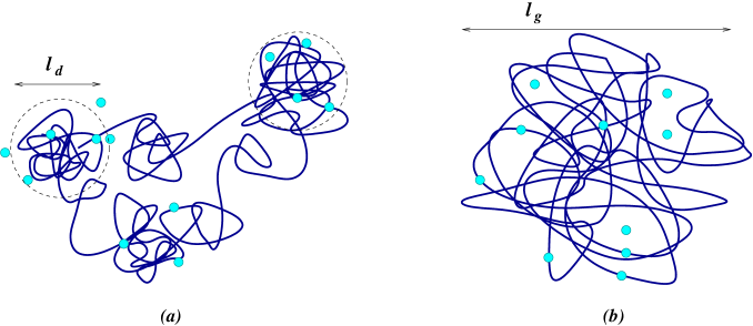
Figure 7: Effect of DNA conformation on the effective diffusion distance: (a) Single globule; (b) Multi-domain conformation.

Considering the microscopic picture one can easily obtain a reasonable estimate of $\tau_{3d}$ as a characteristic time of 3D diffusion across the nucleoid (the region of a bacterial cell to which the DNA is confined). The corresponding diffusion length depends on the conformation of the DNA molecule. Indeed, if the DNA molecule was a single homogeneous globule, there would be a single relevant length scale, which is the molecule characteristic size $l_{\rm m}$ (the gyration radius). On the other hand, as Fig. 7 shows, diffusion of a protein molecule inside a more realistic non-homogeneous multi-domain molecule involves at least one additional length scale $l_{\rm d}$, which is a characteristic size of a domain. These two lengths may differ by a factor of $\sim 10$ Neidhardt et al. (1996), making the ratio of the resulting diffusion times $\tau^{m}_{3d}/\tau^{d}_{3d}\sim 10^{2}$. In the original problem (a single protein molecule searching for a single site on the DNA), the search process is dominated by the larger time-scale, since at least few domains must be explored before the target site is located. However, there are usually about $10^{2}$ TF molecules present in a cell, so it is reasonable to assume that the domains are scanned in parallel, making the inter-domain transfer processes irrelevant.

Appendix D: Stability requirement

In fact, it is not hard to estimate analytically the $(\sigma/k_{B}T)$ ratio for a genome of length $M$ such that the probability of binding to the lowest site is comparable to the probability of binding to the rest of the genome. , i. e. their contributions to the partition function are of the same order of magnitude. The partition sum for the Gaussian energy level statistics is.

$$\Omega = \frac{M}{\sqrt{2\pi\sigma^{2}}}\int_{-\infty}^{\infty}e^{-\beta U-U^{2}/(2\sigma^{2})}dU=Me^{\beta^{2}\sigma^{2}/2}\sim$$ (48)

$$\sim \exp\left[-\beta U_{\rm min}\right]\sim\exp\left(\beta\sigma\sqrt{2\ln M}\right)$$

so that for $M=10^{6}$

$$\sigma\sim k_{B}T\sqrt{2\ln M}\simeq 5~{}k_{B}T.$$ (49)

Strictly speaking, for a large though finite set of energy levels, the integration limits are cut off at $\pm\sigma\sqrt{2\ln M}$ so that for $\beta\sigma\gg\sqrt{\ln M}$ the partition function is dominated by the lower edge of the distribution. The estimate for $\beta\sigma$ gives therefore the crossover value between the regime of multiple-site contribution to $\Omega$ and the regime with single-site domination.

If $N_{p}$ proteins are searching and binding a single target site, then the probability of being occupied is given by

$$P(N_{p})=1-\left(1-P_{b}\right)^{N_{p}}\approx N_{p}P_{b}$$ (50)

where $P_{b}$ is the probability of the site being occupied by a single protein (eq 19 of the paper) and approximation is for $P_{b}<<1/N_{p}$. As evident from Fig 4b, requirement of the rapid search is satisfied if $P_{b}(\sigma/T\approx 1)\sim 10^{-5}$. An unfeasible amount of $10^{4}$ copies of a single TF are required to saturate such weak binding site.

Appendix E: Energy Gap

Large energy gap between the cognate site $\vec{s}_{c}$ and the bulk of genomic sites would solve the paradox of rapid search and stability. One may seek parameters $\epsilon(j,s)$ of the energy function

$$U(\vec{s}=s_{i},..s_{i+l-1})=\sum_{j=1}^{l}\epsilon(j,s_{j}),$$ (51)

to maximize the energy gap by minimizing the Z-score

$$Z(\vec{s}_{c})=\frac{U(\vec{s}_{c})-\langle U\rangle}{\sigma},$$ (52)

where averaging and variance is taken over all possible sequences of length $l$ (or over genomic words of length $l$). It’s easy to see that $Z(\vec{s}_{c})$ is minimal if

$$\epsilon^{\rm opt}(j,s)=-\delta(s,{s_{c}}_{j})$$ (53)

where $\delta(x,y)$ is Kronecker delta. For $K$ types of nucleotides assuming their equal frequency in genome we obtain the maximal reachable energy gap of

$$Z^{\rm min}=-\sqrt{lK}.$$ (54)

For $K=4$ and $l\approx 8$ we get $Z^{\rm min}\approx-5$. For the genome of $10^{6}-10^{7}$bp the energy spectrum of the genomic DNA ends at $Z\approx-5$. While sufficient to provide stability of the bound complex (see main text), such energy gap is unable to resolve the search-stability paradox.

Appendix F: Diffusion in water and in cytoplasm

The diffusion coefficient of a protein molecule in water can be estimated as Landau and Lifshitz (1987)

$$D\simeq\frac{k_{B}T}{3\pi\eta d},$$ (55)

where $d$ is the diameter of the molecule and $\eta$ is the water viscosity. Setting $\eta\sim 10^{-2}~{}\rm{g/(sec\cdot cm)}$ and $d\sim 10~{}\rm{nm}$, we obtain at room temperature

$$D\sim 10^{2}~{}\mu\rm{m^{2}/sec}.$$ (56)

Diffusion coefficient measurements for GFP in $E.~{}coli$ Elowitz et al. (1999) produce values of about $1-10~{}\mu\rm{m^{2}/sec}$. This difference in diffusion coefficients may account for more than order of magnitude difference in the theoretically calculated and measured target location times.

References

- Abkevich et al. (1994) Abkevich, V., A. Gutin, and E. Shakhnovich, 1994, Biochemistry 33, 10026.
- Akke (2002) Akke, M., 2002, Curr. Opin. Struct. Biol. 12, 642.
- Bell and Lewis (2000) Bell, C. E., and M. Lewis, 2000, Nat. Struct. Biol. 7, 209.
- Bell and Lewis (2001) Bell, C. E., and M. Lewis, 2001, Curr. Opin. Struct. Biol. 11, 19.
- Berg and von Hippel (1987) Berg, O. G., and P. H. von Hippel, 1987, J. Mol. Biol. 193, 723.
- Berg et al. (1981) Berg, O. G., R. B. Winter, and P. H. von Hippel, 1981, Biochemistry 20, 6929.
- Bouchaud and Georges (1990) Bouchaud, J. P., and A. Georges, 1990, Phys. Rep. 195, 127.
- Bruinsma (2002) Bruinsma, R. F., 2002, Physica A 313, 211.
- Clarke et al. (1991) Clarke, N., L. Beamer, H. Goldberg, C. Berkower, and C. Pabo, 1991, Science 254, 267.
- Derrida (1981) Derrida, B., 1981, Phys. Rev. B 24, 2613.
- Dyson and Wright (2002) Dyson, H. J., and P. E. Wright, 2002, Curr. Opin. Struct. Biol. 12, 54.
- Elowitz et al. (1999) Elowitz, M. B., M. G. Surette, P. E. Wolf, J. B. Stock, and S. Leibler, 1999, J. Bacteriol. 181, 197.
- Erie et al. (1994) Erie, D., G. Yang, H. Schultz, and C. Bustamante, 1994, Science 266, 1562.
- Finkelstein and Ptitsyn (2002) Finkelstein, A., and O. Ptitsyn, 2002, Protein Physics (Academic Press).
- Flyvbjerg et al. (2002) Flyvbjerg, H., F. Jülicher, P. Ormos, and F. David (eds.), 2002, Physics of bio-molecules and cells (Springer-Verlag Heidelberg), volume 75 of Les Houches, chapter 1.
- Gerland et al. (2002) Gerland, U., J. D. Moroz, and T. Hwa, 2002, Proc. Natl. Acad. Sci. USA 99, 12015.
- Goldhirsh and Gefen (1986) Goldhirsh, I., and Y. Gefen, 1986, Phys. Rev. A 33, 2583.
- Grillo et al. (1999) Grillo, A. O., M. P. Brown, and C. A. Royer, 1999, J. Mol. Biol. 287, 539.
- Gutin et al. (1998) Gutin, A., A. Sali, V. Abkevich, M. Karplus, and E. Shakhnovich, 1998, J. Chem. Phys. 108, 6466.
- von Hippel and Berg (1989) von Hippel, P. H., and O. G. Berg, 1989, J. Biol. Chem. 264, 675.
- Hopfield (1974) Hopfield, J. J., 1974, Proc. Natl. Acad. Sci. USA 71, 4135.
- Hughes (1995) Hughes, B. D., 1995, Random Walks and Random Environments (Clarendon Press).
- Kalodimos et al. (2004) Kalodimos, C., N. Biris, A. Bonvin, M. Levandoski, M. Guennuegues, R. Boelens, and R. Kaptein, 2004, Science 305, 386.
- Kalodimos et al. (2002) Kalodimos, C. G., R. Boelens, and R. Kaptein, 2002, Nat. Struct. Biol. 9, 193.
- Kalodimos et al. (2001) Kalodimos, C. G., G. E. Folkers, R. Boelens, and R. Kaptein, 2001, Proc. Natl. Acad. Sci. USA 98, 6039.
- Kim et al. (1987) Kim, J. G., Y. Takeda, B. W. Matthews, and W. F. Anderson, 1987, J. Mol. Biol. 196, 149.
- Landau and Lifshitz (1987) Landau, L., and E. Lifshitz, 1987, Fluid Mechanics (Butterworth-Heinemann).
- Levy et al. (2004) Levy, Y., P. Wolynes, and J. Onuchic, 2004, Proc Natl Acad Sci U S A 101, 511.
- Lewis et al. (1996) Lewis, M., G. Chang, N. C. Horton, M. A. Kercher, H. C. Pace, M. A. Schumacher, R. G. Brennan, and P. Lu, 1996, Science 271, 1247.
- Lomakin and Frank-Kamenetskii (1998) Lomakin, A., and M. Frank-Kamenetskii, 1998, J Mol Biol 276, 57.
- Luscombe et al. (2000) Luscombe, N. M., S. E. Austin, H. M. Berman, and J. M. Thornton, 2000, Genome Biol. 1, 1.
- Mirny and Shakhnovich (2001) Mirny, L., and E. Shakhnovich, 2001, Annu Rev Biophys Biomol Struct 30, 361.
- Murthy and Kehr (1989) Murthy, K. P. N., and K. W. Kehr, 1989, Phys. Rev. A 40, 2082.
- Neidhardt et al. (1996) Neidhardt, F. C., R. Curtiss, and E. C. Lin (eds.), 1996, Escherichia Coli and Salmonella (ASM Press), chapter 12.
- O’Neil et al. (1990) O’Neil, K., R. Hoess, and W. DeGrado, 1990, Science 249, 774.
- Pande et al. (2000) Pande, V., A. Grosberg, and T. Tanaka, 2000, Rev. Mod. Phys. 72, 259 314.
- Richter and Eigen (1974) Richter, P. H., and M. Eigen, 1974, Biophys. Chem. 2, 255.
- Riggs et al. (1970a) Riggs, A. D., S. Bourgeois, and M. Cohn, 1970a, J. Mol. Biol. 53, 401.
- Riggs et al. (1970b) Riggs, A. D., H. Suzuki, and S. Bourgeois, 1970b, J. Mol. Biol. 48, 67.
- Schumacher et al. (1994) Schumacher, M. A., K. Y. Choi, H. Zalkin, and R. G. Brennan, 1994, Science 266, 763.
- Shimamoto (1999) Shimamoto, N., 1999, J. Biol. Chem. 274, 15293.
- Shoemaker et al. (2000) Shoemaker, B., J. Portman, and P. Wolynes, 2000, Proc Natl Acad Sci U S A 97, 8868.
- Slutsky et al. (2004) Slutsky, M., M. Kardar, and L. Mirny, 2004, Phys. Rev. E 69, 061903.
- Spolar and Record (1994) Spolar, R. S., and M. T. Record, 1994, Science 263, 777.
- Stormo and Fields (1998) Stormo, G. D., and D. S. Fields, 1998, Trends Biochem. Sci. 23, 109.
- Takeda et al. (1989) Takeda, Y., A. Sarai, and V. M. Rivera, 1989, Proc. Natl. Acad. Sci. USA 86, 439.
- Uversky (2002) Uversky, V. N., 2002, Protein Sci. 11, 739.
- Williams et al. (2001) Williams, P., D. Pollock, and R. Goldstein, 2001, J Mol Graph Model 19, 150.
- Winkler et al. (1993) Winkler, F., D. Banner, C. Oefner, D. Tsernoglou, R. Brown, S. Heathman, R. Bryan, P. Martin, K. Petratos, and K. Wilson, 1993, EMBO J 12, 1781.
- Winter et al. (1989) Winter, R. B., O. G. Berg, and P. H. von Hippel, 1989, Biochemistry 20, 6961.
- Wright and Dyson (1999) Wright, P. E., and H. J. Dyson, 1999, J. Mol. Biol. 293, 321.