Space-irrelevant scaling law for
fish school sizes

Abstract

Universal scaling in the power-law size distribution of pelagic fish schools is established. The power-law exponent of size distributions is extracted through the data collapse. The distribution depends on the school size only through the ratio of the size to the expected size of the schools an arbitrary individual engages in. This expected size is linear in the ratio of the spatial population density of fish to the breakup rate of school. By means of extensive numerical simulations, it is verified that the law is completely independent of the dimension of the space in which the fish move. Besides the scaling analysis on school size distributions, the integrity of schools over extended periods of time is discussed.

1 Introduction

Pelagic fish commonly cruise as a school. As they migrate about in a limited space, interaction between schools can occur so that two of them encounter and aggregate, or a large school splits itself into two smaller schools, or more. The continuation of these interaction processes of fission and fusion may eventually lead to a fat-tailed school-size distribution. Bonabeau and Dagorn (1995) found power law in school-size distributions of tropical tuna. The power-law distributions of school sizes are quite general for pelagic fishes (Niwa, 1998), and quantitative analyses are now in progress (Bonabeau et al., 1998, 1999; Niwa, 2003).

A model of school aggregation proposed by Bonabeau and Dagorn (1995) is based on a physical model of particle aggregation, i.e. open systems showing power-law cluster-size distributions (Takayasu, 1989). Bonabeau and Dagorn’s (1995) model is briefly sketched as follows. Simulated fish schools move between sites on coarse-grained zones of space, and aggregate when they meet. School splitting is replaced by (re)injection process: a certain fraction of each school is separated from the school; the fish that have left their school are reinjected as individuals (i.e. one-sized schools) into the system, while the total number of individuals is kept fixed. Bonabeau and Dagorn (1995) obtained a truncated power law with exponent $-3/2$ in the mean-field case of the model, in which schools can move from any site to any other site.

The mean-field assumption might not always be adequate, because there are spatial constraints on movement. Although the ocean is three-dimensional, fish may not fully use their spatial environment. Pelagic fish movement generally takes place in a horizontal (two-dimensional) space. They are limited in depth by physiological constraints, and do not dive into the deeps. Additionally, pelagic fish schools are concentrated in the vicinity of the front which is the contact zone and collision line of two oceanic currents (Uda, 1938). For instance, skipjack schools, Euthynnus vagans (Lesson), aggregate in the interfacial region between the cold subarctic and warm subtropic waters (Uda, 1936). They are constrained to move effectively in a one-dimensional space. In the presence of a fish aggregating device (FAD), which is a drifting log or an artificial device designed to attract fish, pelagic fish do not make full use of the three-dimensional oceanic space and are concentrated in the vicinity of a FAD (a point), so that the space dimension effectively decreases to less than one.

Bonabeau et al. (1998, 1999) predicted spatial effects, i.e. the dimensional reduction that the power-law exponent of fish school-size distributions is modified from the mean-field case of their model when the dimension of the space is taken into account: the absolute value of the exponent, in a version of their model on a $d$-dimensional lattice (schools hop to neighboring sites only), decreases when the space dimension $d$ decreases.

Recently, Niwa (2003) analyzed some existing data for various species in terms of a school-size histogram of the population of fish. $N$ fish swimming together form an $N$-sized school. The school-size distribution $W(N)$ is proportional to the observed number of $N$-sized schools; the size histogram of the population is then represented by $P(N)=NW(N)$, which is proportional to the fraction of fish in $N$-sized schools to total population. He reported that the distribution $P$ is an exponentially thin-tailed distribution, and, the distribution $W$ follows a power-law decay with exponent $-1$ and is truncated at a cut-off size. A simple stochastic-differential-equation model was proposed to explain the observed power-law behavior, and the predictions of the model were found to be consistent with empirical data. A remarkable feature is “scaling”: all the empirical distributions collapse onto a single curve if the data are plotted in terms of scaled coordinates with the mean value of a histogram $P(N)$, for all various species and for all environmental factors including the above mentioned space dimension. Note that the power-law distribution $W$ does not have a well-defined mean; contrary the rapidly decreasing distribution $P$ has a well-defined mean.

The empirically determined power-law exponents of school-size distributions for specific data sets range from 0.7 to 1.8 (Niwa, 1998; Bonabeau et al., 1999). Fat-tailed school-size distributions are necessarily truncated because the population is finite. This truncation of the power-law regime might lead to a “wrong” estimation of the exponent. I make use of the data collapse to extract the “right” exponent. I here propose a finite-size scaling (FSS) form (Binder and Heermann, 1988) for the size distribution $W(N)$ on the assumption that the distribution decays with the truncated power-law form with biologically universal exponent. The power-law exponent of distribution $W$ is determined by experimentally fitting the FSS relation to achieve the best data collapse. It is investigated by simulating the school system of pelagic fish whether or not the dimension of the space in which fish swim is relevant to the power-law exponent. FSS for fish school sizes is elucidated through the competition between two processes in the interacting school system: aggregation and splitting of schools.

In addition, it is numerically investigated how long a school stays together, i.e. neither merges with any other schools nor breaks up. The behavioral algorithms governing school formation and dynamics have been extensively studied [e.g. Inada and Kawachi (2002) and references cited therein]. Studies of the integrity of schools, however, are very few [e.g. Lester et al. (1985) or Bayliff (1988) for experimental studies; Niwa (1996) for a modeling approach]. Numerical simulations of fish-school aggregation suggest conjectures about real situations that could be tested by observations.

2 The Data

The enlarged sets of the data in Niwa (2003) for school-size distributions of pelagic fishes are analyzed (summarized in Table 1). The ways of estimating school sizes of pelagic fishes were catch per set by a purse seine or acoustic surveys. Catch-per-set data are expressed in school weight (in metric tons). Acoustic-survey data are expressed in dimensional size of a school (e.g. vertical thickness in meters), which can be reduced to the biomass in a school: the school biomass is proportional to the vertical cross-section, the square of vertical thickness, or the square of diameter of a school (Squire, 1978; Anderson, 1981; Misund, 1993; Niwa, 1995; Misund and Coetzee, 2000).

Table 1: Species analyzed.

	Species	cut-off size${}^{\mbox{\scriptsize a}}$	Data sources
$\vartriangle$	Northern anchovy	$15.67\cdot\Delta N$	Smith (1970)${}^{\mbox{\scriptsize c}}$.
	Engraulis mordax ${}^{\mbox{\scriptsize b}}$		Acoustic survey
$\bullet$	Japanese sardine	$6.45\cdot(\Delta N/2)$ to	Hara (1990).
	Sardinops melanosticta	$23.77\cdot(\Delta N/2)$	22 acoustic surveys
$\square$	Tropical tuna${}^{\mbox{\scriptsize d}}$	$11.69\cdot\Delta N$	Bonabeau et al. (1999).
	(free swimming)		Data from fisheries
$\lozenge$	Tropical tuna${}^{\mbox{\scriptsize d}}$	$4.80\cdot\Delta N$	Bonabeau et al. (1999).
	(caught in the vicinity of FADs)		Data from fisheries
$\circ$	Herring Clupea harengus	$7.24\cdot\Delta N$ to	Reid et al. (2000).
		$10.88\cdot\Delta N$	4 acoustic surveys
${}^{\mbox{\scriptsize a}}$The cut-off size of power-law distribution is calculated by Eq.(9). $\Delta N$ denotes
the class width of frequency data of school sizes, and will be omitted.
${}^{\mbox{\scriptsize b}}$possibly including Trachurus symmetricus, Sarda chiliensis, Scomber japonicus,
and Sardinops sagax.
${}^{\mbox{\scriptsize c}}$Data are cited in Anderson (1981).
${}^{\mbox{\scriptsize d}}$Three species (Thunnus albacares, Katsuwonus pelamis, and Thunnus obesus)
are mixed.

Let $R$ be the dimensional size (vertical thickness or diameter acoustically measured) of a steady moving $N$-sized school. The following relation between dimensional and social sizes holds in a statistical sense:

$$R=(\mbox{constant})\times N^{\nu},$$ (1)

where $\nu=0.5$. The prefactor is supposed to be constant for each data set (i.e. each survey). It may depend on the species and vary with regions, seasons and years in which fish schools are surveyed. The acoustic-survey data are transformed into a social size histogram as follows

$$W(N)\mbox{d}N\propto W(R)R^{1/\nu-1}\mbox{d}R,$$ (2)

where $W$ denotes the school-size distribution density.

The data are given by the set $\left\{\left.\left(N_{i},W_{i}\right)\right|i=1,2,\ldots,n\right\}$. $W_{i}\Delta N$ reads the frequency of school sizes which lie within the $i$-th class $\left[N_{i}-\Delta N/2,N_{i}+\Delta N/2\right)$, where $\Delta N$ denotes the class width and the $i$-th class mark is given by $N_{i}=(i-0.5)\cdot\Delta N$. From now on, to simplify the expression, we will omit $\Delta N$ (or $\Delta N/2$ for Japanese sardine) in mathematical formulae for processing empirical data, that is, such unit of school size is introduced as $\Delta N=1$ ($\Delta N=2$ for Japanese sardine). A school of unit size contains a certain number of individuals, for instance, $\Delta N$ should be a number of fish correspond to 1000 kilograms for tropical tuna.

As with fisheries such as fishing by a purse seiner, such major events (i.e. large catches) can be regarded as unusual events of great magnitude lying on the tail of a distribution comprising events that are mostly of much smaller magnitude. Figure 1 shows the school-size distribution for Japanese sardine Sardinops melanosticta, which was from the acoustic survey off southeastern Hokkaido covering the period July 30 – August 6 in 1982 [Hara (1990); the same data are available in Hara (1984)]. A traditional, widely used Gauss statistics says that finding sardine schools ranging from 18 to 20 meters in vertical thickness should only occur about once every $10^{9}$ detections of schools. In other words, it is not the real world! Aquatic observations actually say that finding such schools occurs about once every 500 detections. The probability that such schools are found is $10^{6}$ times large!

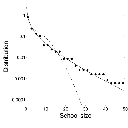
Figure 1: Comparison of the empirical data with Gaussian distribution (broken line). Japanese sardine schools were surveyed in the summer in 1982 (Hara, 1990). The trial Gaussian distribution has the variance $M_{2}$ equal to the second moment of empirical distribution ($M_{2}=\sum_{i}N_{i}^{2}W_{i}/\sum_{i}W_{i}=46.8$). The normalization of Eq.(17), $\sum_{i=1}^{n}N_{i}W_{i}=\langle N\rangle_{P}$, is chosen, where $\langle N\rangle_{P}$ is given by Eq.(9). The Gaussian distribution is consistently normalized. The probability to find sardine schools ranging from 18 to 20 meters in vertical thickness (denoted by $p_{19}$) is $2.0\times 10^{-3}$ from the data. The Gaussian distribution gives $p_{19}=8.1\times 10^{-10}$. The social size of such sardine schools as $R\in[18,20)$ in meters are transformed into $N\in[42,50)$. The solid line shows the size distribution proposed by Niwa (2003), with $\langle N\rangle_{P}=11.7$ calculated from the data. Plotted on semilogarithmic scale.

2.1 Finite-size Scaling

The size distributions of pelagic fish schools follow a power law $W(N)\propto N^{-\beta}$ up to a cut-off size

$$L=\frac{\sum_{i=1}^{n}N_{i}^{1+\beta}W_{i}}{\sum_{i=1}^{n}N_{i}^{\beta}W_{i}}.$$ (3)

In order to characterize the effects of the finite population size on the truncation of power-law distribution, a finite-size scaling hypothesis is used: the distribution depends on $N$ only through the ratio $N/L^{A}$,

$$\tilde{W}(N;L)\mbox{d}N=L^{-B}F\left(N/L^{A}\right)\mbox{d}\left(N/L^{A}\right),$$ (4)

where $F$ is a universal function independent of system (population) size, and $\tilde{W}_{i}=W_{i}/\sum_{i=1}^{n}N_{i}^{\beta}W_{i}$. The prefactor $L^{-B}$ is required to ensure the normalization

$$\sum_{i=1}^{n}N_{i}^{\beta}\tilde{W}_{i}=1.$$ (5)

School sizes are assumed to obey FSS with biologically universal exponents $A$ and $B$ for a wide spectrum of both pelagic species and environmental conditions. The normalization Eq.(5) together with the postulated universal function $F(x)$ gives

$$\int_{0}^{\infty}L^{\beta A-B}x^{\beta}F(x)\mbox{d}x=1.$$ (6)

It then follows that

$$\beta=\frac{B}{A},$$ (7)

because all powers of $L$ must cancel out. From the FSS hypothesis, it is expected that when $\tilde{W}(N)L^{A+B}$ is plotted against $N/L^{A}$ with correct parameters $A$ and $B$ all the empirical data should collapse onto a single curve. The power-law exponent of fish school-size distributions, $\beta$, is then evaluated through FSS analysis. Besides Eq.(7), if FSS is valid the value of $A$ is $1$.

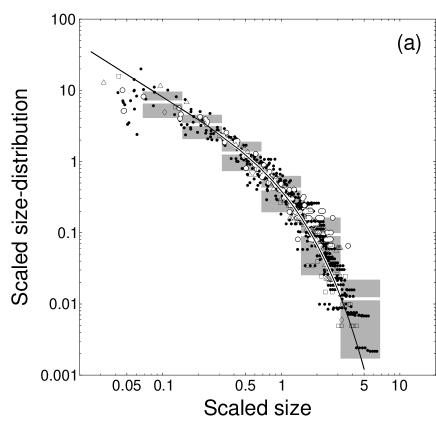
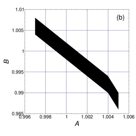
Figure 2: FSS analysis of the empirical data (summarized in Table 1). (a) FSS plot of the school-size distribution on double-logarithmic scale. Here $y=\tilde{W}L^{A+B}$ is plotted versus $x=N/L^{A}$ with $A=B=1$. The bins are chosen equally spaced on a logarithmic scale as $x\in\left[10^{-1+(k-0.5)/3},10^{-1+(k+0.5)/3}\right)$ with $k=0,1,\ldots,5$. For each bin two-dimensional variance $\epsilon$ is calculated (the rectangle in gray reads the interval $\overline{y}\pm\sigma_{y}$; the mean $\overline{y}$ is indicated by the slit). The solid line is a prediction of the mean-field theory (Niwa, 2003). (b) The region of the $AB$-plane in which the minimum of the mean of two-dimensional variance exists. The mean of two-dimensional variance, $\overline{\epsilon}$, takes a minimum $\overline{\epsilon}_{\mbox{\scriptsize min}}$ for the right choice of $(A,B)$. The minimum is found with the precision i.e. width of the minimum, $\Delta\epsilon=10^{-3}$ in black region ($\Delta\epsilon/\overline{\epsilon}_{\mbox{\scriptsize min}}\approx 2.58\times 10^{-3}$). The values of the parameters lie in the intervals $A=1.001\pm 0.004$ and $B=0.997\pm 0.011$. The value of $B/A$ is the estimate of the power-law exponent $\beta$, and therefore $\beta=0.996\pm 0.015$. Experimentally fitting the parameters $A$ and $B$ to achieve a good data collapse yields the values $A=B=\beta=1$, which are precisely the values of the mean-field case of the proposed model.

Let us search for the values of $A$ and $B$ that do the best job of placing all the data points on a single curve. To do this, the $x$-axis is divided into bins (Fig.2a), and the parameters are estimated at values that minimize the mean of two-dimensional variance

$$\epsilon=\left(\sigma_{x}/\overline{x}\right)^{2}+\left(\sigma_{y}/\overline{y}\right)^{2}$$ (8)

(Lillo et al., 2002, 2003), where $\sigma$ denotes the standard deviation, and $\overline{x}$ and $\overline{y}$ denote the mean, and the $x$-axis is chosen as $x=N/L^{A}$, and the $y$-axis represents $y=\tilde{W}(N)L^{A+B}$. The mean of two-dimensional variance, $\overline{\epsilon}$, is a measure to determine the goodness of collapse. Figure 2b displays the set of pairs $(A,B)$ in which the minimum of the mean of two-dimensional variance, $\overline{\epsilon}_{\mbox{\scriptsize min}}$, is guaranteed to lie. A good data collapse can be obtained by using the values $A\approx 1$ and $B\approx 1$. The power-law exponent derived from the FSS collapse is $\beta\approx 1$. The resulting plot is shown in Fig.2a. The figure confirms the FSS hypothesis, since all the data collapse onto a single curve. The school-size distribution follows a power-law decay with exponent $-1$, and is truncated at the cut-off size that equals the mean of another distribution of the school system, $P_{i}=N_{i}W_{i}$, i.e. the size histogram of the fish population. The distribution $P$ decays rapidly for large $N$, and has a well-defined mean

$$\langle N\rangle_{P}=\frac{\sum_{i=1}^{n}N_{i}^{2}W_{i}}{\sum_{i=1}^{n}N_{i}W_{i}}.$$ (9)

Two competing processes, mixing and splitting of schools, determine the school-size distribution. The spatial density of fish population conditions the mixing rate of schools. The population density of a given species differs among regions, seasons and years. The breakup rate of schools of a given species may vary depending on environmental conditions, e.g. the lack of food may reduce school stability (Morgan, 1988). Figure 2a shows that the power-law exponent “$-1$” is robust, while the cut-off size of linear power law varies (Table 1). The data-collapse implies that the breakup rate and the population density do not affect the power-law exponent but the cut-off size. This indicates that the power-law exponent is universal, and hence the overall shape of the distribution may result from a simple underlying aggregation mechanism. Moreover, as a consequence of the quite good data-collapse, the empirical data do not support the dimensional reduction, because the “effective” dimension is related to biological or environmental conditions. In the following two sections we will numerically examine whether or not space dimension influences the power-law exponent.

3 The Model

A stationary equilibrium system of a fixed population size (number of individuals, denoted by $\Phi$) is considered in which fish schools break up and merge with other schools. Let us investigate the aggregation process in a discretized space and time. There are $s$ sites on the lattice space $\Omega$. On every site there is at most one school of simulated fish. Let $N(j,t)$ be the size of the school on site $j$ at the $t$-th time step. At each discrete time step, each school hops to a new site or breaks up into pairs of schools of various sizes possible. If more than two schools happen to hop onto one site, they coalesce into a single school with the size equal to the sum of the sizes of the incident schools. Assume binary splitting independent of school size. Each school with a size greater than or equal to 2 splits into a pair of schools with a probability $p$ at each time step. The probability $p$ for a school to split per time step (i.e. breakup rate) is independent of its size, and the sizes of splitting schools are uniformly distributed: a probability for an $N$-sized school to split into $M$- and $(N-M)$-sized schools is represented by

$$K_{\mbox{\scriptsize b}}(N|M,N-M)=K_{\mbox{\scriptsize b}}(N)=\frac{p}{N-1},$$ (10)

for $N\geq 2$.

The aggregation process can be represented by the following stochastic equation for $N(j,t)$:

$$N(j,t+1)=\sum_{k\in\Omega}M_{jk}(t)N(k,t),$$ (11)

where $M_{jk}(t)$ is a stochastic variable. If the school on site $k$ does not break, $M_{jk}(t)$ is equal to 1 when the school jumps to site $j$ and equal to 0 otherwise ($M_{ik}(t)=0$ for $i\neq j$). If an $N$-sized school on site $k$ breaks up into two schools of sizes $mN$ and $(1-m)N$ jumping to sites $j$ and $j^{\prime}$, respectively, then we have $M_{jk}(t)=m$, $M_{j^{\prime}k}(t)=1-m$, and the others vanish ($M_{ik}(t)=0$ for $i\neq j,j^{\prime}$), where $m$ is also a stochastic variable uniformly distributed in $(0,1)$ on condition that $mN$ is an integer. $M_{jk}(t)$ must be normalized as

$$\sum_{j\in\Omega}M_{jk}(t)=1,$$ (12)

for $\forall k$ and $\forall t$, which guarantees the conservation of population.

In the mean-field case of the model, at each time step, all schools move towards a randomly selected site, which corresponds to the migration of the high potential speed of fish, e.g. free-swimming tuna. They may move to any site with equal probability $1/s$. In spatial model of school aggregation, schools hop to neighboring sites only. In a version of the model on a $d$-dimensional lattice, they may move to each of $2d$ neighboring sites with equal probability $1/2d$. If a school on site $j$ breaks, one of splitting schools remains at the site $j$ and the other hops to neighboring sites.

Table 2: Parameters used in simulations. Monte-Carlo simulations of fish school aggregation on the lattice space of $s=2^{18}$ sites with periodic boundary have been conducted by using Mersenne Twister (Matsumoto and Nishimura, 1998), a pseudorandom number generator, on Scientific Computing System of MAFFIN, Tsukuba Japan.

	breakup rate $p$	population $\Phi$	$\langle N\rangle_{P}$  [1D; 2D; mf] ${}^{\mbox{\scriptsize a}}$
$\blacklozenge$	0.02	$2^{14}$	1.72; 4.23; 8.97
$\blacksquare$	0.02	$2^{15}$	3.08; 8.57; 17.87
$\blacktriangle$	0.02	$2^{16}$	6.39; 18.57; 38.40
$\bullet$	0.02	$2^{17}$	13.44; 39.41; 74.25
$\bigstar$	0.02	$2^{18}$	28.39; 73.83; 157.61
$\lozenge$	0.01	$2^{17}$	19.63; 68.59; 146.61
$\square$	0.03	$2^{17}$	10.98; 27.00; 48.51
$\vartriangle$	0.04	$2^{17}$	9.13; 20.29; 37.03
$\circ$	0.1	$2^{17}$	5.54; 9.41; 13.94
${}^{\mbox{\scriptsize a}}$ $\langle N\rangle_{P}$ was computed from simulation results after $2^{17}$ time steps
for one- (1D), two-dimensional (2D), and mean-field (mf) cases.

3.1 Finite-size Scaling

Simulations have been performed with the coarse-grained zones of $s=2^{18}$ sites, simulation run $=2^{17}$ time steps, and parameters summarized in Table 2. The initial school-system configurations are taken to be random distribution of eight-sized schools on the lattice space. Numerical results are shown in the next section (in Fig.6b an FSS collapse of $W(N)$ for the two-dimensional case is depicted). We search for the values of $A$ and $B$ that place all of the simulated distributions most accurately on a single curve. The parameters $A$ and $B$ derived via the minimization of the measure $\overline{\epsilon}$ to quantify FSS collapse are summarized in Table 3. In the one- and two-dimensional cases, there is a clear minimum for $A\approx B\approx 1$. Therefore, the power-law exponent extracted from numerical simulations reads $\beta\approx 1$, and does not depend on the dimensionality $d$. This may cause one surprise, because such exponents depend on the dimensionality as the critical exponents for scaling behavior in wide varieties of physical phenomena, e.g. magnetization, specific heat, size of a polymer, and so on.

Table 3: Summary of exponents $A$, $B$, and $\beta$. The exponents are evaluated at values in the listed ranges with the precision $\Delta\epsilon=10^{-3}$ through FSS analyses of empirical data and simulated distributions at the last of run for different population sizes and breakup rates in one- and two-dimensional cases.

	$A$	$B$	$\beta$	$\Delta\epsilon/\overline{\epsilon}_{\mbox{\scriptsize min}}$
data	$1.001\pm 0.004$	$0.997\pm 0.011$	$0.996\pm 0.015$	$2.58\times 10^{-3}$
1D	$0.998\pm 0.012$	$1.020\pm 0.026$	$1.022\pm 0.037$	$2.93\times 10^{-3}$
2D	$0.992\pm 0.011$	$1.019\pm 0.026$	$1.028\pm 0.037$	$1.01\times 10^{-2}$
mf${}^{\mbox{\scriptsize a}}$	1	1	1	—
${}^{\mbox{\scriptsize a}}$ predicted values of the mean-field theory (Niwa, 2003).

4 The Scaling Law

The cut-off size of power-law distribution (equal to $\langle N\rangle_{P}$) results from variable individual behavior (i.e. breakup rate $p$) and fluctuating population density (denoted by $\rho$). The FSS collapse suggests that the school-size distribution $W(N)$ depends on $N$, $p$, and $\rho$ only through the variable $x=N/\langle N\rangle_{P}$. Numerical simulations reveal that $\langle N\rangle_{P}$ depends linearly on the spatial population density and inversely on the breakup rate (Fig.3):

$$\langle N\rangle_{P}=c\rho/p.$$ (13)

The prefactor $c$ must have dimensions of $[\mbox{length}]^{d}/[\mbox{time}]$, and it is indeed proportional to the ratio of the coalesce rate to the spatial density of schools, as discussed later.

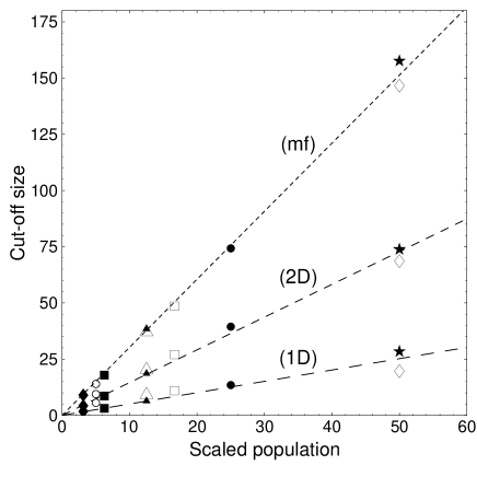
Figure 3: Plot of $\langle N\rangle_{P}$ against the scaled population size (numerical results from simulations summarized in Table 2). The abscissa represents $\rho/p$, the coarse-grained population density $\rho\;(=\Phi/s)$ divided by breakup rate $p$. Broken lines are fits with slopes 0.503 (1D), 1.46 (2D), and 3.03 (mf), respectively, which give the prefactor $c$ in Eq.(13).

The frequencies of the amount of $N$-sized schools ($N=1,2,\ldots,\Phi$) at the last of simulation run in the two-dimensional case, ${\hat{W}}(N;\rho,p)$, are shown in Figs.4a and 5a for a given breakup rate $p$ and a given coarse-grained spatial population density $\rho=\Phi/s$, respectively. The frequencies are normalized as

$$\sum_{N=1}^{\Phi}N{\hat{W}}(N)=\Phi.$$ (14)

Figure 4: Simulated school-size distribution (2D) with the breakup rate $p=0.02$, $s=2^{18}$ sites after $2^{17}$ time steps. (a) Frequencies ${\hat{W}}(N)$ of $N$-sized schools in the two-dimensional simulations with various population sizes summarized in Table 2. The straight line illustrates a general trend, i.e. the power-law behavior with exponent $-1$. (b) The frequencies in Fig.4a re-plotted with $W^{\prime}={\hat{W}}(N)\rho$ as a function of variable $N^{\prime}=N/\rho$. The scaling causes a shift of the curves in Fig.4a that depend on $\rho$. All the distribution collapse onto a single curve. Plotted on double-logarithmic scale.

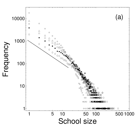
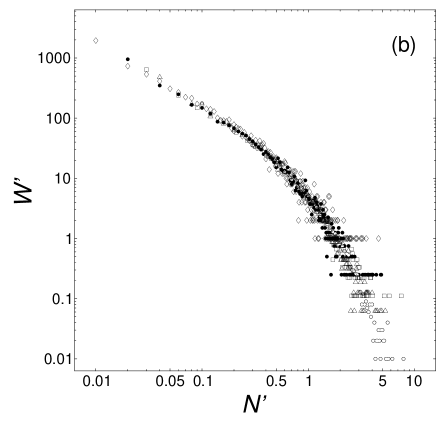
Figure 5: Simulated school-size distribution (2D) with the population density $\rho=0.5$ (population $\Phi=2^{17}$), $s=2^{18}$ sites after $2^{17}$ time steps. (a) Frequencies ${\hat{W}}(N)$ of $N$-sized schools in the two-dimensional simulations with various breakup rates summarized in Table 2. The straight line illustrates a general trend, i.e. the power-law behavior with exponent $-1$. (b) The frequencies in Fig.5a re-plotted with $W^{\prime}=10^{-4}{\hat{W}}(N)p^{-2}$ as a function of variable $N^{\prime}=Np$. The scaling causes a shift of the curves in Fig.5a that depend on $p$. All the distribution collapse onto a single curve. Plotted on double-logarithmic scale.

Examining Fig.4a closely shows that for fixed breakup rate $p$ but increasing population density $\rho$, the range of the power-law regime increases: the cut-off size of power law scales with $\rho$ as depicted in Fig.4b. The FSS form (4) with $A=B=1$ together with Eq.(13) reads

$${\hat{W}}(N;\rho,p=0.02)\mbox{d}N=N^{-1}g(N/\rho)\mbox{d}\left(N/\rho\right),$$ (15)

where $g(x)$ is a scaling function.

Similar behavior is seen in Fig.5a when $p$ varies. As $p$ increases, the length of the power-law region reduces: the cut-off size of power law scales with $1/p$ as depicted in Fig.5b, i.e.

$${\hat{W}}(N;\rho=0.5,p)\mbox{d}N=pN^{-1}g^{\prime}(Np)\mbox{d}\left(Np\right),$$ (16)

where $g^{\prime}(x)$ is a scaling function. Each resulting graph shows that all the distributions collapse onto a single curve (Figs.4b and 5b).

The same results can be obtained with one-dimensional case of the model, and its mean-field case as well.

4.1 The Unified School-size Law

Equation (13) implies that the population density must appear as a ratio to the breakup rate in the scaling analysis, and the breakup rate vice versa. For instance, the following normalization is appropriate for the scaling analysis of school based data:

$$\sum_{i=1}^{n}N_{i}W_{i}=\langle N\rangle_{P}.$$ (17)

The FSS form of Eq.(4) then suggests that the linear dependence of $\langle N\rangle_{P}$ on the population size gives $B=1$. By arguments discussed below, the FSS form (4) expresses the unified scaling law for school sizes. The scaling behavior of the school-size distribution is described by two independent parameters: the population density $\rho$ and the breakup rate $p$. One of the important results of the model is that a single parameter $\langle N\rangle_{P}$ is sufficient to describe the scaling behavior, i.e., the two scaling relations of Eqs.(15) and (16) are unified into Eq.(4) because of Eq.(13).

To understand the unified scaling law for school sizes, it is essential to see what determines the cut-off size of power law. The cut-off size is determined by the competition between breakup and coalescence of schools. The coalescence is regulated by the spatial number-density of schools resulting from a balance of the population density and the breakup rate of schools. Equation (13) is then fundamental to unify the two scaling laws (15) and (16). Let us trace the size change of the school a certain individual (named “A”) rides. Let $\phi$ be the coarse-grained density of schools (i.e. number of schools per site), and, $\lambda$ the probability for a school to coalesce with other schools per time step (i.e. coalescence rate). Then the expected increment and decrement of the size of “A”-riding school (denoted by $N_{\mbox{\scriptsize A}}$) are $c_{0}(\rho/\phi)\lambda$ (accompanied by a constant factor $c_{0}$) and $pN_{\mbox{\scriptsize A}}/2$, respectively, at each time step of coarse-grained simulation [$\rho/\phi$ reads an (apparent) average size of fish schools]. The expected size-change of “A”-riding school per time step, $\Delta N_{\mbox{\scriptsize A}}$, obeys

$$\Delta N_{\mbox{\scriptsize A}}=c_{0}\left(\frac{\rho}{\phi}\right)\lambda-\frac{p}{2}N_{\mbox{\scriptsize A}}.$$ (18)

The ratio $(\lambda c_{0}\rho/\phi)/(p/2)$, therefore, gives the expected size of “A”-riding school in the stationary state, which is equivalent to the value of $\langle N\rangle_{P}$ by definition. Thus, the fundamental equation (13) is approved:

$$\langle N\rangle_{P}=2c_{0}\frac{\lambda}{\phi}\cdot\frac{\rho}{p},$$ (19)

where $c_{0}$ is just a number independent of space dimension, fit giving $1.54\pm 0.02$ in the simulations (Fig.6a). The values of the ratio of $c$ to $\lambda/\phi$ for one-, two-dimensional, and mean-field cases are estimated at 3.09, 3.11, and 3.07, respectively, which all exhibit the similar value independent of the case of the model. The space dimension is irrelevant to the (reduced) prefactor $c_{0}$. (How does one a priori obtain the specific value of the dimensionless quantity $c_{0}$ within the model setting?)

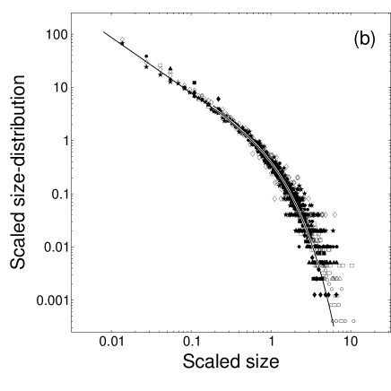
Figure 6: Unified scaling law for school sizes. (a) $\langle N\rangle_{P}$ versus the re-scaled population size. The data in Fig.3 are re-plotted in terms of re-scaled coordinate: the abscissa represents $(\lambda/\phi)\rho/p$. Factors $\lambda/\phi$ for one- ($\blacktriangle$), two-dimensional ($\blacklozenge$), and mean-field ($\bullet$) cases are estimated at 0.163, 0.469, and 0.985, respectively. The solid line is fit with slope 3.08. (b) Simulated school-size distribution plotted on double-logarithmic scale (2D). The data in Figs.4 and 5 are re-plotted with $y=c\rho p^{-1}W(N)$ as a function of the scaling variable $x=N/c\rho p^{-1}$, where $c=1.46$. The frequency distributions are normalized as $\sum_{N=1}^{\Phi}NW(N)=c\rho/p$. The re-scaled distributions collapse onto one another. The data collapse is equivalent to the FSS plot with $A=B=1$ in Eq.(4). The solid line is a prediction of the mean-field theory (Niwa, 2003).

Thus the above two scaling relations can be unified and reduced to

$$W(N;\rho,p)\mbox{d}N=N^{-1}G\left(N/(2c_{0}\lambda\phi^{-1})\rho p^{-1}\right)\mbox{d}\left(N/(2c_{0}\lambda\phi^{-1})\rho p^{-1}\right),$$ (20)

with normalization $\sum_{N=1}^{\Phi}NW(N)=(2c_{0}\lambda\phi^{-1})\rho p^{-1}$, which corresponding to Eq.(17). A scaling function $G(x)$ has a strong drop for $x>1$. To verify this law, the simulated data in Figs.4 and 5 are re-plotted in terms of re-scaled coordinates where the $x$-axis is chosen as $x=N/(2c_{0}\lambda\phi^{-1})\rho p^{-1}$, and the $y$-axis represents $y=(2c_{0}\lambda\phi^{-1})\rho p^{-1}W(N)$. The resulting graph is shown in Fig.6b. The data collapse is very good, implying a unified law for school sizes.

The same numerical results can be obtained with one-dimensional case of the model. Besides, the data-collapse in its mean-field case is depicted in Fig.4 in Niwa (2003). Therefore, the unified scaling law, Eq.(20), holds independently of the space dimension: space does not influence a linear power-law behavior with a crossover to an exponential decay around $\langle N\rangle_{P}$. Figure 7 in the next section showing the comparison of the empirical school-size distribution with simulated distributions in one-, two-dimensional, and mean-field cases directly verifies the irrelevance of space in the scaling law for fish school sizes.

5 The Integrity of Schools

The cut-off size in the scaling law results from the ability of a school to maintain its integrity over only a certain amount of time: $\langle N\rangle_{P}$ varies in proportion as the coalescence rate, and inversely as the breakup rate [see Eq.(19)]. The proposed numerical approach to fish school-size distribution may answer yet another challenging question: how schools split.

Let us analyze the school sizes of Japanese sardine acoustically surveyed in the summer in 1982 (the same data set as Fig.1). Transect sampling was carried out for a length of $\xi=$ 1211.208 kilometers in a survey area of $\omega=26904\;\mbox{km}^{2}$, and 1522 schools (denoted by $\mu$) were observed. The average (horizontal) interception-length of schools was $\overline{\ell}=$ 20.9 meters. We now apply Buffon’s needle problem to the estimation of the dimensional size and the spatial number-density of fish schools (Doi, 1979).

Assume the shape of fish schools be horizontally disk-like with the (average) diameter $\overline{R}$. Let $a$ be the average of inter-school distance, so that the number density of schools, $\tilde{\phi}$, is given by $a^{-2}$. Imagine a disk (instead of a needle) dropping on a lined sheet of paper. The probability of the disk hitting one of the lines is $P_{\mbox{\scriptsize disk}}=\overline{R}/a$. Then the average interception-length of schools is calculated as $\overline{\ell}={\pi(\overline{R}/2)^{2}}/a$. Since we expect to observe one school for a transect sample interval of length $\delta=\xi/\mu$, the average length of successive detections of schools, the strip of width $a$ and length $\delta$ contains $1/P_{\mbox{\scriptsize disk}}$ schools, i.e. $\tilde{\phi}a\delta=1/P_{\mbox{\scriptsize disk}}$. Accordingly, $\delta/a=a/\overline{R}$ is obtained. Then the average diameter of schools and the average inter-school distance are given by

$$\overline{R}=\sqrt[3]{\frac{16}{\pi^{2}}\overline{\ell}^{2}\delta}=82.6\;\mbox{m},$$ (21)

and

$$a=\sqrt[3]{\frac{4}{\pi}\overline{\ell}\delta^{2}}=256.4\;\mbox{m},$$ (22)

respectively. Thus the fine-grained spatial number-density of schools, $\tilde{\phi}$, is estimated at $15.2\;\mbox{km}^{-2}$.

We now return to the coarse-grained model of school aggregation. Let the average diameter of schools, $\overline{R}$, be the lattice constant. The data are normalized to the coarse-grained density of schools, $\phi=\tilde{\phi}\overline{R}^{2}=0.104$:

$$s^{-1}\sum_{i}{\hat{W}}_{i}=\phi,$$ (23)

where $s=2^{22}$ sites ($\approx\omega/\overline{R}^{2}$). Then the coarse-grained population density is estimated at

$$\rho=s^{-1}\sum_{i}N_{i}{\hat{W}}_{i}=0.415,$$ (24)

where unit is half the class width of size histogram (per site). The empirical data yield $\langle N\rangle_{P}=11.7$.

Table 4: Summary of simulations for Japanese sardine schools. Monte-Carlo simulations have been performed with coarse-grained zones of $s=2^{22}$ sites, $\Phi=1.74\times 10^{6}$ individuals, and simulation run $=2^{17}$ time steps.

	$p$	$\phi$ ${}^{\mbox{\scriptsize a}}$	$\langle N\rangle_{P}$ ${}^{\mbox{\scriptsize a}}$	half-life $T$ ${}^{\mbox{\scriptsize b}}$	$\lambda$	$p_{T}\;(=p\cdot T)$
1D ($\vartriangle$)	0.0179	0.105	11.7	23.5	$1.15\times 10^{-2}$	0.421
2D ($\lozenge$)	0.0516	0.092	13.6	7.55	$4.02\times 10^{-2}$	0.390
mf ($\circ$)	0.107	0.109	10.9	3.45 (3.29)${}^{\mbox{\scriptsize c}}$	$9.41\times 10^{-2}$	0.369
${}^{\mbox{\scriptsize a}}$computed from simulation results at the last of run
${}^{\mbox{\scriptsize b}}$Unit is simulation time step.
${}^{\mbox{\scriptsize c}}$predicted by $(\ln 2)/(p+\phi)$ with $\phi=0.104$ (evaluated value from empirical data)

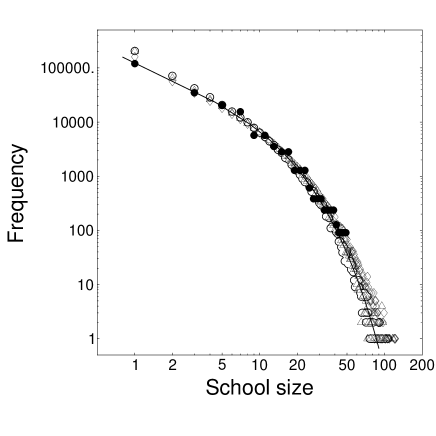
Figure 7: Empirical school-size distribution of sardine observed in the summer in 1982 ($\bullet$), same as Fig.1 but with normalization Eq.(23), compared with simulated distributions after $2^{17}$ time steps in one- ($\vartriangle$), two-dimensional ($\lozenge$), and mean-field ($\circ$) cases of the model. The simulated distributions are in good agreement with empirical data. Different plots for the empirical observation and the numerical simulations fall onto one another. The solid line is a prediction of the mean-field theory [Eq.(11) in Niwa (2003)], with normalization $\Phi\cdot\left[\langle N\rangle_{P}\int_{0}^{\infty}\exp\left[-x\left(1-e^{-x}/2\right)\right]\mbox{d}x\right]^{-1}=1.31\times 10^{5}$, consistent with Eq.(24), where $\langle N\rangle_{P}=11.7$. The simulation parameters are summarized in Table 4. Plotted on double-logarithmic scale.

Now we can numerically experiment on the school size distribution with the population $\Phi=s\rho$ and the breakup rate $p$ listed in Table 4. The breakup probability $p$ at each simulation time step is estimated at $c\rho/\langle N\rangle_{P}$, by using Eq.(13) with prefactors resulting from simulations (Fig.3). A one-sized school of simulated fish ($N=1$) is considered as an atomic object, which contain a certain number of fish correspond to half the class width of frequency data of sardine school sizes observed in the wild. Starting from random initial configurations of eight-sized schools on the lattice, the coarse-grained simulations imitate the fine-grained situation of the real-world, as shown in Fig.7. The remarkable consistency between the empirical data and the model’s prediction unambiguously describes that the space dimension cannot be relevant to the scaling exponent of power-law school-size distribution.

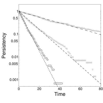
Figure 8: Persistency of simulated sardine schools in one- ($\vartriangle$), two-dimensional ($\lozenge$), and mean-field ($\circ$) cases of the model. Shown is a ratio of the number of schools maintaining their integrity over a certain amount of time steps of simulation run without coalescing or splitting. Broken lines depict the exponential decays with rates $p+\lambda=0.0294$ (1D), $0.0918$ (2D), and $0.201$ (mf) fitting the numerical results, respectively (unit: per time step). The simulation parameters are summarized in Table 4. Plotted on semilogarithmic scale.

Let us investigate the dynamic properties from the numerical results. There are two competing processes in the interacting school system: breakup and coalescence. The disintegration behavior of fish schools consists of these two processes. The breakup and coalescence rates, therefore, combine into the probability of disintegration per unit time per school, which gives the half-life $T$ as its reciprocal:

$$T=\frac{\ln 2}{p+\lambda}.$$ (25)

After time $T$, the number of schools maintaining their integrity is half of the original number (Fig.8). In the mean-field case of the model, the coalescence probability per simulation time step is given by the density of schools, $\lambda=\phi$, which is tested numerically. The half-life of simulated fish schools is calculated in Table 4. The breakup probability per half-life, $p_{T}\;(=p\cdot T)$, obtained for each case (1D/2D/mf) exhibits the similar value independent of the case of the model. Therefore, if the half-life of sardine school is experimentally determined in the wild [e.g. Lester et al. (1985) or Bayliff (1988) for skipjack tuna], we can estimate the breakup rate and the coalescence rate in the wild at $p_{T}/T$ and $(\ln 2-p_{T})/T$, respectively, with numerically predicted value $p_{T}$.

6 Discussions

Data collapse is a way of establishing the scaling in fish school-size distributions. I have extracted the power-law exponent of size distributions via a minimization of a measure to quantify the nature of finite-size scaling collapse, in contrast to the ‘best-by-eye’ data-collapse method. The number $W(N)$ of $N$-sized schools decays with the truncated power-law form with exponent $-1$, and the power-law cut-off scales with $\langle N\rangle_{P}$, which is a well-defined mean of the population distribution among school sizes, $NW(N)$. In order to explain the observed scaling property, I have chosen a stationary equilibrium model, contrary to a stationary non-equilibrium system of Bonabeau et al.’s (1995, 1998, 1999) model. It has been found that the scaling law for school sizes of pelagic fish is completely independent of the dimension of the space in which the fish move: the space dimension is irrelevant to the power-law exponent of size distributions. This result is contrary to common knowledge in physics that the critical exponents characterizing the scaling behavior observed in phase transitions depend on the dimensionality. The model of school aggregation does not perfectly mirror the interacting school system in the wild (e.g. the size of a school may be relevant to its breakup probability), yet the numerically simulated result conforms almost perfectly to the empirical data. This is a consequence of universality (Stanley, 1995).

The scaling law supports the view that the power-law distribution of fish schools is a self-organized critical phenomenon (Bak, 1996; Jensen, 1998), not merely a reflection of an exponential distribution of population among school sizes, because only critical processes exhibit data-collapse (Yeomans, 1992; Bak et al., 2002, Christensen et al., 2002), known as scaling in critical phenomena. The interacting school system is naturally attracted to the critical value of the spatial number-density of fish schools, without any external adjustment being necessary. In the system there are two competing processes, coalescence and breakup, and the critical density depends crucially on the interplay between the coalescence and breakup time scales. If the school density becomes greater (or less) than the critical value, this increased (or decreased) density in turn increases (or decreases) the probability of coalescence, leading to a shift toward less (or greater) density until it reverts to the critical value.

The relation between dimensional and social sizes of pelagic fish schools, Eq.(1), gives another scaling law for the school size, which is analogous to that used in polymer physics (de Gennes, 1979). What is universal in this law is the exponent $\nu$: it is the same for all schools, supposed to be independent of not only environmental conditions but also species. What is non-universal here is the prefactor. It depends on the details of interactions between individuals. If we want to understand the properties of schooling configurations, the first step is to explain the existence and the value of the exponent $\nu$. The second step is to account for the constant that multiplies $N^{\nu}$, and this involves delicate studies on local properties within a school. In the first stage, the school size $N$ (in number or biomass) must be measured for different values of dimensional size $R$ and compare them. Finding the exact value of $N$ for a given school is not an easy task, whereas acoustic surveys for pelagic species are extensively performed.

By contraries, the exponent $\nu$ may be estimated by hypothesizing FSS in the school-size distribution of pelagic species. Assume the scaling relation, Eq.(1), and choose the suitable value of $\nu$ to achieve the best data-collapse in the FSS analysis, while a dimensional size histogram for acoustic-survey data is transformed into a social size histogram by using Eq.(2). Once the scaling relation between dimensional and social sizes of pelagic fish schools is established, the precision in the stock assessment will be largely improved.

References

- Anderson (1981) Anderson, J. J., 1981. A stochastic model for the size of fish schools. Fish. Bull. 79, 315–323.
- Bak (1996) Bak, P., 1996. How Nature Works. Springer-Verlag, New York.
- Bak et al. (2002) Bak, P., Christensen, K., Danon, L., Scanlon, T., 2002. Unified scaling law for earthquakes. Phys. Rev. Lett. 88, 178501-1–178501-4., doi:10.1103/PhysRevLett.88.178501.
- Bayliff (1988) Bayliff, W., 1988. Integrity of schools of skipjack tuna, Katsuwonus pelamis, in the eastern Pacific Ocean, as determined from tagging data. Fish. Bull. 86, 631–643.
- Binder and Heermann (1988) Binder, K., Heermann, D. W., 1988. Monte Carlo Simulation in Statistical Physics. Springer-Verlag, Berlin.
- Bonabeau and Dagorn (1995) Bonabeau, E., Dagorn, L., 1995. Possible universality in the size distribution of fish schools. Phys. Rev. E 51, R5220–R5223.
- Bonabeau et al. (1998) Bonabeau, E., Dagorn, L., Fréon, P., 1998. Space dimension and scaling in fish school-size distributions. J. Phys. A: Math. Gen. 31, L731–L736.
- Bonabeau et al. (1999) Bonabeau, E., Dagorn, L., Fréon, P., 1999. Scaling in animal group-size distributions. Proc. Natl. Acad. Sci. USA 96, 4472–4477.
- Christensenk et al. (2002) Christensen, K., Danon, L., Scanlon, T., Bak, P., 2002. Unified scaling law for earthquakes. Proc. Natl. Acad. Sci. USA 99, suppl. 1, 2509–2513., doi:10.1073/pnas.012581099.
- de Gennes (1979) de Gennes, P.-G., 1979. Scaling Concepts in Polymer Physics. Cornell University Press, Ithaca.
- Doi (1979) Doi, T., 1979. Measurements and statistics in marine ecology. Mathematical Sciences, No. 198, pp. 7–12.
- Hara (1984) Hara, I., 1984. Distribution and school size of Japanese sardine in the waters off the southeastern coast of Hokkaido on the basis of echo sounder surveys. Bull. Tokai Reg. Fish. Res. Lab., No. 113, pp. 67–78.
- Hara (1990) Hara, I., 1990. Stock Assessment and Migration of Japanese Sardine Schools in the Waters Off the Southeastern Coast of Hokkaido. Ph.D. Thesis, Kyoto University, Kyoto (Japan).
- Inada and Kawachi (2002) Inada, Y., Kawachi, K., 2002. Order and flexibility in the motion of fish schools. J. Theor. Biol. 214, 371–387., doi:10.1006/jtb.2001.2449.
- Jensen (1998) Jensen, H. J., 1998. Self-Organized Criticality. Cambridge University Press, Cambridge (UK).
- Lester et al. (1985) Lester, R. J. G., Barnes, A., Habib, G., 1985. Parasites of skipjack tuna, Katsuwonus pelamis: fishery implications. Fish. Bull. 83, 343–356.
- Lillo et al. (2002) Lillo, F., Farmer, J. D., Mantegna, R. N., 2002. Single curve collapse of the price impact function for the New York Stock Exchange. preprint cond-mat/0207428 at
- Lillo et al. (2003) Lillo, F., Farmer, J. D., Mantegna, R. N., 2003. Master curve for price-impact function. Nature 421, 129–130.
- Matsumoto and Nishimura (1998) Matsumoto, M., Nishimura, T., 1998. Mersenne Twister: a 623-dimensionally equidistributed uniform pseudorandom number generator. ACM Trans. on Modeling and Computer Simulation 8(1), 3–30.
- Misund (1993) Misund, O. A., 1993. Abundance estimation of fish schools based on a relationship between school area and school biomass. Aquat. Living Resour. 6, 235–241.
- Misund and Coetzee (2000) Misund, O. A., Coetzee, J., 2000. Recording fish schools by multi-beam sonar: potential for validating and supplementing echo integration recordings of schooling fish. Fish. Res. 47, 149–159.
- Morgan (1988) Morgan, M. J., 1988. The effect of hunger, shoal size and the presence of a predator on shoal cohesiveness in bluntnose minnows, Pimephales notatus Rafinesque. J. Fish. Biol. 32, 963–971.
- Niwa (1995) Niwa, H.-S., 1995. Configurational statistics of fish schools with reference to collective motion, in: Fundamental Theories of Deterministic and Stochastic Models in Mathematical Biology. Cooperative Research Report, Inst. Stat. Math., Tokyo, No. 76, pp. 132–143.
- Niwa (1996) Niwa, H.-S., 1996. Mathematical model for the size distribution of fish schools. Computers Math. Applic. 32 (11), 79–88.
- Niwa (1998) Niwa, H.-S., 1998. School size statistics of fish. J. Theor. Biol. 195, 351–361.
- Niwa (2003) Niwa, H.-S., 2003. Power-law versus exponential distributions of animal group sizes. J. Theor. Biol. 224, 451–457., doi:10.1016/S0022-5193(03)00192-9.
- Reid et al. (2000) Reid, D., Scalabrin, C., Petitgas, P., Masse, J., Aukland, R., Carrera, P., Georgakarakos, S., 2000. Standard protocols for the analysis of school based data from echo sounder surveys. Fish. Res. 47, 125–136.
- Smith (1970) Smith, P. E., 1970. The horizontal dimensions and abundance of fish schools in the upper mixed layer as measured by sonar, in: Farquhar, G. B. (Ed.), Proceedings of the International Symposium on Biological Sound Scattering in the Ocean, Maury Cent. Ocean Sci., Dep. Navy., Washington, D.C., pp. 563–591.
- Squire (1978) Squire Jr., J. L., 1978. Northern anchovy school shapes as related to problems in school size estimation. Fish. Bull. 76, 443–448.
- Stanley (1995) Stanley, H. E., 1995. Power laws and universality. Nature 378, 554.
- Takayasu (1989) Takayasu, H., 1989. Steady-state distribution of generalized aggregation system with injection. Phys. Rev. Lett. 63, 2563–2565.
- Uda (1936) Uda, M., 1936. Locality of fishing centre and shoals of “Katuwo,” Euthynnus vagans (Lesson), correlated with the contact zone of cold and warm currents. Bull. Jpn. Soc. Sci. Fish. 4, 385–390.
- Uda (1938) Uda, M., 1938. Researches on “Siome” or current rip in the seas and oceans. Geophys. Mag. 11, 307–372.
- Yeomans (1992) Yeomans, J. M., 1992. Statistical Mechanics of Phase Transitions. Oxford University Press, Oxford.