Clone-array pooled shotgun mapping and sequencing:
design and analysis of experiments

Abstract.

This paper studies sequencing and mapping methods that rely solely on pooling and shotgun sequencing of clones. First, we scrutinize and improve the recently proposed Clone-Array Pooled Shotgun Sequencing (CAPSS) method, which delivers a BAC-linked assembly of a whole genome sequence. Secondly, we introduce a novel physical mapping method, called Clone-Array Pooled Shotgun Mapping (CAPS-MAP), which computes the physical ordering of BACs in a random library. Both CAPSS and CAPS-MAP construct subclone libraries from pooled genomic BAC clones.

We propose algorithmic and experimental improvements that make CAPSS a viable option for sequencing a set of BACs. We provide the first probabilistic model of CAPSS sequencing progress. The model leads to theoretical results supporting previous, less formal arguments on the practicality of CAPSS. We demonstrate the usefulness of CAPS-MAP for clone overlap detection with a probabilistic analysis, and a simulated assembly of the Drosophila melanogaster genome. Our analysis indicates that CAPS-MAP is well-suited for detecting BAC overlaps in a highly redundant library, relying on a low amount of shotgun sequence information. Consequently, it is a practical method for computing the physical ordering of clones in a random library, without requiring additional clone fingerprinting. Since CAPS-MAP requires only shotgun sequence reads, it can be seamlessly incorporated into a sequencing project with almost no experimental overhead.

1. Introduction

In a hierarchical approach to large genome sequencing, one first breaks many genome copies into random fragments. A library is constructed by cloning the fragments, typically as Bacterial Artificial Chromosome inserts (BACs). Some BACs in the library are selected for complete sequencing. Each selected BAC sequence is assembled individually using the shotgun method: a subclone library is prepared by cloning short fragments of the BAC. Subsequently, sequence reads are produced from a sufficient number of randomly chosen subclones. The reads are assembled algorithmically into the BAC sequence. An alternative to the hierarchical, or clone-by-clone, strategy is the whole-genome shotgun approach WGS, which employs a few (essentially 1–3) subclone libraries prepared from the entire genome, without resorting to an intermediate BAC library. The main advantage of the whole-genome approach is that it eliminates the need to prepare tens of thousands of subclone libraries to sequence a mammalian genome. However, it is generally an inadequate strategy for finishing the assembly of such large repeat-rich genomes. For a review of contemporary sequencing methodologies, see, e.g., Sequencing.review.

A new BAC-based sequencing strategy, called Clone-Array Pooled Shotgun Sequencing (CAPSS), was proposed recently CAPSS. CAPSS assembles the complete sequences of individual BACs as does the clone-by-clone approach, but requires a much smaller number of subclone library preparations. The strategy is currently being applied for the first time on a genome scale in the context of sequencing the honey bee genome. This paper provides the theory for the design and analysis of pooling-based genome projects. It also introduces the CAPS-MAP method for physical mapping, and transversal pooling designs for both CAPSS and CAPS-MAP, thereby laying the theoretical foundation for pooling-based genome-scale sequencing projects.

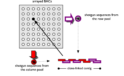
Figure 1. CAPSS strategy for arrayed BACs. DNA extracted from each clone is pooled together with other clones in the same row and column. Subclone libraries are prepared from the pools, and shotgun sequences are collected from the sublibraries. Sequences are assembled into contigs. If a contig contains sequences from a row and a column pool’s sublibrary, the contig is assigned to the BAC at the intersection of the row and the column.

In a clone-by-clone approach, BACs are sequenced independently: one subclone library is constructed for every clone. In contrast, DNA from BACs are pooled together in a CAPSS approach, and subclone libraries are prepared from the pools. A CAPSS experiment is designed so that the number of subclone libraries is much smaller than the number of clones, yet the pooling design enables the assembly of individual clone sequences. In what follows, by pooled shotgun (CAPS) sequences we mean shotgun sequence reads collected from a subclone library that was constructed using pooled BACs. For the computational aspects of sequence assembly, pooled shotgun sequences are random subsequences originating from a set of clone sequences.

The original CAPSS proposal of CAPSS relied on a simple rectangular design defined by an array layout of BACs (Figure 1). The pools correspond to the rows and columns. An array layout reduces the number of shotgun library preparations to the square root of the number of BACs when compared to clone-by-clone sequencing. This reduction can be important in case of a mammalian genome, for which even a minimally overlapping tiling path contains between twenty and thirty thousand clones human.genome.

This paper has two goals. First, after pointing out some shortcomings of the original CAPSS proposal, we propose algorithmic and experimental improvements that make CAPSS a viable option for sequencing a set of BACs. Specifically, we apply transversal pooling designs to increase the accuracy of CAPSS, which we previously developed for the PGI method of comparative physical mapping that also uses pooled shotgun sequencing PGI.conf. We provide the first probabilistic model of CAPSS sequencing progress. The model leads to theoretical results supporting previous, less formal arguments on the practicality of CAPSS.

The paper’s second goal is to introduce the Clone-Array Pooled Shotgun Mapping (CAPS-MAP) method to detect clone overlaps in a random BAC library. The information on clone overlaps is used to compute the physical ordering of clones in the library, without requiring additional clone fingerprinting. CAPS-MAP operates in the same experimental framework as CAPSS. It needs only shotgun sequences, which makes it a cost-effective method that can be seamlessly integrated into a sequencing project with very little experimental overhead. We demonstrate the usefulness of CAPS-MAP for clone overlap detection with a probabilistic analysis. In addition to the theoretical results, we illustrate the method’s performance in a simulated project using the Drosophila genome assembly.

2. Transversal designs

It was proposed by CAPSS that CAPSS be used in hybrid projects, combining whole-genome shotgun (WGS) and pooled shotgun (CAPS) sequences. The motivation is that the pooled shotgun sequences can provide the localization information for the whole-genome shotgun sequences so that the latter can be used for a clone-linked assembly. After WGS and CAPS sequences from a set of pools are assembled into contigs, the contigs need to be mapped to individual BACs. There are a few challenges to contig mapping. We mention here three main problems: false negatives, ambiguities, and false mapping. A false negative refers to a situation where a BAC is not sampled in a pool it is included in, due to the low number of CAPS sequences collected. A false negative for a simple rectangular design means that no contigs can be mapped to the BAC. Ambiguities and false mappings are caused by overlapping clones, or more generally, by clones that have highly similar regions. The mapping of a contig is ambiguous if it is not possible to decide which clones the contig should be assigned to, in cases where two or more clone sets are equally likely choices for the mapping. False mapping occurs when an insufficient number of CAPS sequences are collected, and a contig that covers overlapping BACs gets assigned to the wrong clone or clone set.

One strategy used to overcome the mapping problems involves transversal pooling designs PGI.conf,CGT. For a transversal design with $n$ pool sets, every clone is included in exactly one pool of each pool set, and any subset with two of those pools uniquely identifies the clone. Half of the pool sets are designated as column pools, and the other half as row pools to realize the design with the help of BAC arrays. Using a transversal double-array design (i.e., one with four pool sets), the same set of BACs is independently arrayed twice. Each of the two resulting arrays contains the same set of BACs. Thus, each BAC ends up being sampled in two column-pools and two row-pools. One of the arrays contains an arbitrary arrangement of BACs, while the other is “reshuffled” relative to the first. More generally, clones can be arranged on $d$ reshuffled arrays using a transversal pooling design with $n=2d$ pool sets.

The number of arrays in a transversal design may be adjusted to allow unambiguous and correct contig mapping for any redundancy in a BAC library. Specifically, it can be shown PGI.conf,CGT that a $d$-array transversal design can accurately resolve BACs at up to $(2d-1)$X redundancy. We previously described and analyzed transversal designs in the context of pooled shotgun experiments PGI.conf and compared their performance to other designs. Even though our analysis was performed for the Pooled Genomic Indexing (PGI) method in the context of comparative physical mapping, the results are generally valid for CAPSS and CAPS-MAP as well. Specifically, our results indicate that transversal designs reduce the frequency of false negatives and false mappings when compared to a simple rectangular design. Furthermore, when compared to other more complicated designs, they achieve an optimal balance between the number of shotgun library preparations and the frequency of contig mapping problems. Transversal designs also enjoy a practical advantage over more complicated combinatorial designs, in that they are readily implemented using existing automated clone arraying technologies.

When a transversal design is used, contig mapping can be implemented very efficiently, based on an algorithm that runs in $O(N+M)$ time for mapping $M$ contigs onto $N$ BACs. Without going into details, the main idea is to first build in $O(N)$ time a hash table that maps pool pairs to BACs. Based on the property of transversal designs that two pools identify a clone, this table contains all pool pairs that identify a unique clone. For each contig, it takes $O(1)$ time using the hash table to either identify the most likely clone set to which the contig can be mapped, or to declare the contig ambiguous.

3. Sequence assembly

This section analyzes CAPSS progress in a hybrid project that uses whole-genome and pooled shotgun sequences. CAPS sequences are collected using a transversal design with $n$ pool sets, i.e., $n/2$ arrays. In order to derive a probabilistic model for such experiments, we introduce some standard simplifying assumptions and the following notations. Assume that every clone has the same length $L$ (100–200 thousand base pairs in practice), and that each shotgun sequence has the same length $\ell$ (e.g., 500 bp). The WGS and CAPS sequences are combined and compared to each other to find overlaps between them. Overlapping sequences form islands. Islands with two or more sequences are contigs. An overlap between two shotgun sequences is detected if it is at least of length $\vartheta\ell$ where $0<\vartheta\leq 1$. Statistics for islands, and gaps between islands are well known LanderWaterman,WendlWaterston. We are interested in statistics for clone-linked contigs, those that are assigned to BACs using the pooling information.

Let $a$ be the coverage by CAPS sequences, i.e., if $F_{\mathrm{p}}$ CAPS sequences are collected, then $a=\frac{F_{\mathrm{p}}\ell}{NL}$ where $N$ is the total number of clones. Let $w$ denote the coverage by WGS sequences, i.e., if $F_{\mathrm{w}}$ WGS sequences are collected, then $w=\frac{F_{\mathrm{w}}\ell}{G}$ where $G$ is the genome length. Notice that $w=0$ is possible. Here we consider the simplest case of assembling the sequence of a single clone that does not overlap with any other clone. Such a clone is covered by a total coverage of $(a+w)$. Although we concentrate on sequencing a particular clone, the transversal design allows the simultaneous sequencing of multiple, possibly overlapping clones by combining WGS sequences with CAPS sequences from many (or even all) pools. Regions of overlapping clones have higher coverage since they are covered by more CAPS sequences than a single clone. The sequencing of overlapping regions progresses thus faster than what is suggested by the statistics for a single clone. We examine the case of assigning contigs to overlapping BACs in §4. Two shotgun sequences from different pools suffice to assign a contig to a single BAC. In a practical setting, it may be advantageous to require more stringent criteria in order to avoid false mappings. Theorem 1 can be readily adapted for such criteria, albeit resulting in bulkier formulas.

Figures 2 and 3 compare different experimental designs based on Theorem 1 and simulations. Figure 2 plots the island statistics from the theorem. It illustrates that for lower coverages (about $c<4$), the ratio of pooled shotgun sequences makes a large difference in the sequencing. This difference is mainly shown in the number of clone-linked contigs, as the contig sizes do not differ much. At large coverage levels, when sequencing is nearly completed, the impact of pooled sequences is less, i.e., WGS sequences can make up for a lower pooled coverage.

Figure 3a shows that while more arrays increase the sequencing success, the improvements are very small after the second array. Notice that if the clones are selected from a minimally overlapping tiling path, then no part of the genome is covered by more than two BACs, and thus two arrays suffice for the unambiguous mapping of all contigs that cover clone overlaps. Figure 3b plots the N50 values. The N50 contig length is the value $l$ such that half of the sequenced nucleotides belong to contigs of length at least $l$. The statistics for all designs converge to those of a non-pooled sequencing project as the coverage increases. In other words, the negative effects of pooling diminish and the project progresses just as without pooling: for example, at total coverage 4–5X, 99% of the clone is sequenced.

Theorem 1.

Let $\sigma=1-\vartheta$ where $\vartheta$ is the fraction of length two shotgun sequences must share in order for the overlap to be detected. Consider a BAC that does not overlap with other clones. Define $c=w+a$, the total coverage. Let $X_{1}=\frac{w+\frac{a}{n}}{c}$, $X_{2}=\frac{w}{c}$, and $Y_{i}=1-(1-e^{-c\sigma})X_{i}$ for $i=1,2$.

1. The expected number of clone-linked contigs covering the clone equals

   (1) $$\frac{L}{\ell}ce^{-c\sigma}p_{\mathrm{link}},$$

   where

   (2) $$p_{\mathrm{link}}=\begin{cases}1-e^{-c\sigma}\biggl{(}n\frac{X_{1}}{Y_{1}}-(n-1)\frac{X_{2}}{Y_{2}}\biggr{)}&\text{if $w>0$;}\\ \frac{1-e^{-a\sigma}}{1+\frac{1}{n-1}e^{-a\sigma}}&\text{if $w=0$.}\end{cases}$$

2. The expected number of shotgun sequences in a clone-linked contig is

   (3) $$F_{\mathrm{link}}=\begin{cases}\frac{e^{c\sigma}}{p_{\mathrm{link}}}\Biggl{(}1-e^{-2c\sigma}\biggl{(}n\frac{X_{1}}{Y_{1}^{2}}-(n-1)\frac{X_{2}}{Y_{2}^{2}}\biggr{)}\Biggr{)}&\text{if $w>0$;}\\ e^{a\sigma}+\frac{1+\frac{1}{n-1}}{1+\frac{e^{-a\sigma}}{n-1}}&\text{if $w=0$.}\end{cases}$$

3. Define

   (4) $$F_{\mathrm{nolink}}=\frac{n\frac{X_{1}}{Y_{1}^{2}}-(n-1)\frac{X_{2}}{Y_{2}^{2}}}{n\frac{X_{1}}{Y_{1}}-(n-1)\frac{X_{2}}{Y_{2}}},$$

   and

   (5) $$\lambda_{\mathrm{CBC}}=\frac{e^{c\sigma}-1}{c}+\vartheta.$$

   The expected length of a clone-linked contig can be written as $\ell\lambda_{\mathrm{link}}$ where $\lambda_{\mathrm{link}}$ is bounded as

   (6) $$\frac{\lambda_{\mathrm{CBC}}-\Bigl{(}F_{\mathrm{nolink}}\sigma+\vartheta\Bigr{)}(1-p_{\mathrm{link}})}{p_{\mathrm{link}}}\leq\lambda_{\mathrm{link}}\leq\frac{\lambda_{\mathrm{CBC}}}{p_{\mathrm{link}}}.$$

   Furthermore, when $\mu=a/c$ is kept constant, $F_{\mathrm{nolink}}$ increases monotonically with $c$ and

   (7) $$\lim_{c\to\infty}F_{\mathrm{nolink}}=\begin{cases}\mu^{-1}\frac{(3n^{2}-3n+1)-\mu(2n^{2}-3n+1)}{(2n^{2}-3n+1)-\mu(n^{2}-2n+1)}&\text{if $w>0$;}\\ \frac{n}{n-1}&\text{if $w=0$.}\end{cases}$$

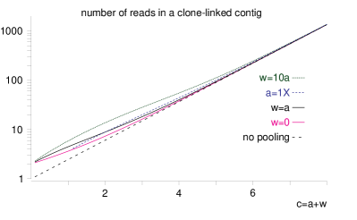
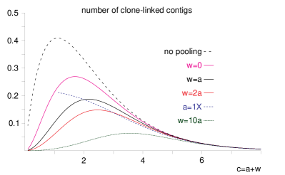
a	b

Figure 2. CAPSS (Theorem 1): clone-linked contig statistics. The values are calculated from Theorem 1 for two-array transversal designs and different pooled coverage levels $a$. Overlaps between shotgun sequences are detected with $\vartheta=0.1$. The number of contigs on the right-hand side is given in multiples of $L/\ell$. The abscissa is the total coverage $c$.

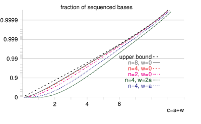
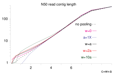
a	b

Figure 3. CAPSS (Theorem 1): sequencing progress. The left-hand side plots the fraction of bases covered by clone-linked contigs as a function of total coverage ($c=a+w$) for different designs. Notice that the improvement from two arrays to four arrays ($n=4$ vs. $n=8$) is marginal. The right-hand side plots the N50 values for different designs with two arrays, as multiples of $\ell$. All values were calculated with shotgun sequence overlap detection $\vartheta=0.1$. The N50 plot was obtained from simulation: each point is an average of 200 measurements.

Proof.

The proof relies on a Poisson process model, following the technique of Waterman. We model the location of the shotgun sequences as a Poisson process with rate $c$. Define $\mu=a/c$, the fraction of CAPS sequences. Every sequence is either a WGS sequence with probability $(1-\mu)$, or comes from each one of the clone’s pools with probability $\mu/n$. First we state the well-known facts LanderWaterman,Waterman about apparent islands, whether or not they are linked to a clone. The event $E$ that a given shotgun sequence is the right-hand end of an apparent island has probability $J=\mathbb{P}E=e^{-c\sigma}$. For the $k$-th read, define $M_{k}$ as the number of reads from its right-hand end until the first gap towards the left. The probability that an island has $j$ sequences in it equals

$${\mathbb{P}}\Bigl{\{}M_{k}=j\Bigm{|}E\Bigr{\}}=(1-J)^{j-1}J.$$

An island can be mapped to a clone if it contains sequences from at least two pools. The probability of mapping the island ending at the $k$-th read (event $D_{k}$) depends on the number of shotgun sequences in the island. Using inclusion-exclusion:

(8) $${\mathbb{P}}\Bigl{\{}D_{k}\Bigm{|}M_{k}=j\Bigr{\}}\\ \begin{aligned} &=1-\sum_{\text{pools}}{\mathbb{P}}\Bigl{\{}\text{CAPS reads from only one pool+WGS}\Bigm{|}M_{k}=j\Bigr{\}}\\ &+(n-1){\mathbb{P}}\Bigl{\{}\text{only WGS reads}\Bigm{|}M_{k}=j\Bigr{\}}\\ &=1-n\Bigl{(}1-\frac{n-1}{n}\mu\Bigr{)}^{j}+(n-1)(1-\mu)^{j}.\end{aligned}$$

By Equation (8), the number of shotgun sequences in a clone-linked island is distributed by the probabilities

(9) $${\mathbb{P}}\Bigl{\{}D_{k},M_{k}=j\Bigm{|}E\Bigr{\}}={\mathbb{P}}\Bigl{\{}D_{k}\Bigm{|}M_{k}=j,E\Bigr{\}}{\mathbb{P}}\Bigl{\{}M_{k}=j\Bigm{|}E\Bigr{\}}\\ \begin{aligned} &=\biggl{(}1-n\Bigl{(}1-\frac{n-1}{n}\mu\Bigr{)}^{j}+(n-1)(1-\mu)^{j}\biggr{)}(1-J)^{j-1}J\\ &=P_{0}(j)-nP_{\mu}^{(n)}(j)+(n-1)P_{\mu}^{(\infty)}(j).\end{aligned}$$

with

(10a) $$P_{0}(j) =(1-J)^{j-1}J;$$

(10b) $$P_{\mu}^{(n)}(j) =\biggl{(}(1-J)\Bigl{(}1-\frac{n-1}{n}\mu\Bigr{)}\biggr{)}^{j-1}J\Bigl{(}1-\frac{n-1}{n}\mu\Bigr{)};$$

(10c) $$P_{\mu}^{(\infty)}(j) =\Bigl{(}(1-J)(1-\mu)\Bigr{)}^{j-1}J(1-\mu).$$

Now, for all $0<z\leq 1$,

(11) $$\sum_{j=1}^{\infty}(1-z)^{j-1}=\frac{1}{z};\quad\sum_{j=1}^{\infty}j(1-z)^{j-1}=\frac{1}{z^{2}}.$$

Using Equation (11),

$${\mathbb{P}}\Bigl{\{}D_{k}\Bigm{|}E\Bigr{\}} =\sum_{j=1}^{\infty}{\mathbb{P}}\Bigl{\{}D_{k},M_{k}=j\Bigm{|}E\Bigr{\}}$$

$$=1-\frac{nJ(1-\frac{n-1}{n}\mu)}{1-(1-J)\Bigl{(}1-\frac{n-1}{n}\mu\Bigr{)}}+\frac{(n-1)J(1-\mu)}{1-(1-J)(1-\mu)}.$$

In Equation (2), $p_{\mathrm{link}}={\mathbb{P}}\Bigl{\{}D_{k}\Bigm{|}E\Bigr{\}}$. Equation (1) follows from the fact that the expected number of shotgun fragments covering the clone equals $cL/\ell$.

By definition of the conditional probability,

$${\mathbb{P}}\Bigl{\{}M_{k}=j\Bigm{|}D_{k},E\Bigr{\}}=\frac{{\mathbb{P}}\Bigl{\{}D_{k},M_{k}=j\Bigm{|}E\Bigr{\}}}{{\mathbb{P}}\Bigl{\{}D_{k}\Bigm{|}E\Bigr{\}}}=\frac{P_{0}(j)-nP_{\mu}^{(n)}(j)+(n-1)P_{\mu}^{(\infty)}(j)}{p_{\mathrm{link}}},$$

where the values can be plugged in from Equations (2) and (10). By Equation (11),

(12) $${\mathbb{E}}\Bigl{[}M_{k}\Bigm{|}D_{k},E\Bigr{]}=\frac{p_{\mathrm{link}}^{-1}}{J}\Biggl{(}1-\frac{nJ^{2}\Bigl{(}1-\frac{n}{n-1}\mu\Bigr{)}}{\Bigl{(}1-(1-J)(1-\frac{n-1}{n}\mu)\Bigr{)}^{2}}+\frac{(n-1)J^{2}(1-\mu)}{\Bigl{(}1-(1-J)(1-\mu)\Bigr{)}^{2}}\Biggr{)},$$

which corresponds to (ii) with $F_{\mathrm{link}}={\mathbb{E}}\Bigl{[}M_{k}\Bigm{|}D_{k},E\Bigr{]}$. It is interesting to notice that when $\mu=1$, in Equation (12),

$$\frac{2}{J(\sigma)}\geq{\mathbb{E}}\Bigl{[}M_{k}\Bigm{|}D_{k},E\Bigr{]}>\frac{1}{J(\sigma)},$$

and that ${\mathbb{E}}\Bigl{[}M_{k}\Bigm{|}D_{k},E\Bigr{]}J^{-1}(\sigma)$ decreases when the coverage $c$ increases.

By Equation (2),

(13) $${\mathbb{P}}\Bigl{\{}\overline{D_{k}}\Bigm{|}E\Bigr{\}}=1-p_{\mathrm{link}}=1-J\frac{1-\Bigl{(}1-J\Bigr{)}\Bigl{(}1-\frac{n-1}{n}\mu\Bigr{)}(1-\mu)}{\biggl{(}1-\Bigl{(}1-J\Bigr{)}\Bigl{(}1-\frac{n-1}{n}\mu\Bigr{)}\biggr{)}\biggl{(}1-\Bigl{(}1-J\Bigr{)}\Bigl{(}1-\mu\Bigr{)}\biggr{)}}.$$

The expected number of shotgun sequences in an island that is not mapped to a clone equals

$${\mathbb{E}}\Bigl{[}M_{k}\Bigm{|}\overline{D_{k}},E\Bigr{]}=\frac{{\mathbb{E}}\Bigl{[}M_{k}\Bigm{|}E\Bigr{]}-{\mathbb{E}}\Bigl{[}M_{k}\Bigm{|}D_{k},E\Bigr{]}{\mathbb{P}}\Bigl{\{}D_{k}\Bigm{|}E\Bigr{\}}}{{\mathbb{P}}\Bigl{\{}\overline{D_{k}}\Bigm{|}E\Bigr{\}}}.$$

Using ${\mathbb{E}}\Bigl{[}M_{k}\Bigm{|}E\Bigr{]}=J^{-1}$ and Equations (12), (2), and (13), we get Equation (4) with the notation $F_{\mathrm{nolink}}={\mathbb{E}}\Bigl{[}M_{k}\Bigm{|}\overline{D_{k}},E\Bigr{]}$.

Let $\ell\lambda_{k}$ be the length of the island ending with the $k$-th sequence. The length of a non-linked island can be bounded as $\ell{\mathbb{E}}\Bigl{[}\lambda_{\mathrm{nolink}}\Bigm{|}\overline{D_{k}},E\Bigr{]}$ with

$$1\leq{\mathbb{E}}\Bigl{[}\lambda_{\mathrm{nolink}}\Bigm{|}\overline{D_{k}},E\Bigr{]}\leq{\mathbb{E}}\Bigl{[}M_{k}\Bigm{|}\overline{D_{k}},E\Bigr{]}\sigma+\vartheta.$$

The bounds of Equation (6) follow from

$${\mathbb{E}}\Bigl{[}\lambda_{k}\Bigm{|}D_{k},E\Bigr{]}=\frac{{\mathbb{E}}\Bigl{[}\lambda_{k}\Bigm{|}E\Bigr{]}-{\mathbb{E}}\Bigl{[}\lambda_{k}\Bigm{|}\overline{D_{k}},E\Bigr{]}{\mathbb{P}}\Bigl{\{}\overline{D_{k}}\Bigm{|}E\Bigr{\}}}{{\mathbb{P}}\Bigl{\{}\overline{D_{k}}\Bigm{|}E\Bigr{\}}},$$

where ${\mathbb{E}}\Bigl{[}\lambda_{k}\Bigm{|}E\Bigr{]}=\lambda_{\mathrm{CBC}}=\frac{J^{-1}-1}{c}+\vartheta$ Waterman. ∎

The value $\lambda_{\mathrm{CBC}}$ in the theorem is the expected island length in a non-pooled sequencing project. By Equation (7), and the fact that $\lim_{c\to\infty}p_{\mathrm{link}}=1$, we have $\lim_{c\to\infty}\lambda_{\mathrm{link}}=\lambda_{\mathrm{CBC}}$ when the ratio of CAPS sequences is kept constant. This limit result is not surprising given that every island can be assigned to a clone with near certainty when the sequence read coverage is large.

4. Clone overlap detection

The key observation for this section is that a transversal design makes it possible to map a contig unambiguously to more than one BAC at once. Now, a contig that is mapped to two clones simultaneously can be viewed as evidence that the two clones overlap. Taking the idea further, an entire set of BACs can be tested for overlaps in this manner, which leads us to the Clone-Array Pooled Shotgun Mapping (CAPS-MAP) method that is described as follows. A redundant collection of random BACs covering a large genome is grouped into subsets of size $q^{2}$. Pooled shotgun sequence reads are collected from each clone group using a transversal design with $d$ arrays of size $q\times q$. Partitioning into subsets may be dictated by the practical concerns of chemistry, biology and robotic automation. For array sizes that are multiples of 8 or 12 or both (yielding standard dimensions of a 96-well microtiter plate), such as $q=24$, or $q=48$, there exist known design.handbook transversal designs. A pooling design with a few ($d=2,3,4$) arrays suffice to compute the physical ordering of BACs in the library, depending on the library’s redundancy and the array sizes. In addition to the CAPS sequences, WGS sequences are used to increase read contig lengths. The shotgun sequences are compared to each other to find the overlaps between them, and are assembled into contigs. Contigs that map unambiguously to more than one clone are taken as evidence that the clones overlap. See Figures 4 and 5 for illustrations. The clone overlap information can then be used to compute the physical ordering of the BACs in the library, and to select a minimal tiling path for complete sequencing, just as if the overlaps were detected using a fingerprinting scheme map.sequenceready.

Theorem 2 considers the case of detecting an overlap between two clones in different clone groups. Similar analyses can be carried out for more general cases with more overlapping clones, or clones in the same clone group, resulting in more cumbersome formulas.

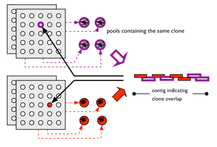
Figure 4. CAPS-MAP detects overlaps between clones by identifying situations where a read contig maps simultaneously to two clones. This figure illustrates a transversal pooling design with two clone groups and two arrays per group. The transversal design guarantees that the intersection of any two pools out of four possible for each BAC (two row and two column pools) uniquely identifies the BAC. Note that overlaps between clones on the same array can also be detected by a transversal design.

Figure 5. Overlaps between clones on the same array can also be detected by a transversal design, even in the presence of false negatives, i.e., situations where a particular BAC is not represented in a particular pool. Specifically, overlap between the two BACs illustrated in the figure is detected despite the fact that each BAC is sampled in only three pools.

Figure 6 plots the overlap detection probabilities in a few scenarios with different amounts of CAPS and WGS sequences. Based on the figure, the probability of detecting an overlap increases exponentially toward 1 with the overlap length. The same exponential behavior is characteristic of clone anchoring methods for overlap detection map.anchor. Consequently, clone contig statistics for CAPS-MAP can be calculated using a clone anchoring model with an appropriate anchoring process intensity. Clone contig statistics can also be estimated using a fingerprinting model LanderWaterman by noticing that clone overlaps above a certain length are detected with near certainty. Figure 6 indicates that using 1X CAPS coverage and 2–5X WGS coverage, BAC overlaps of more than 20000 bp are detected almost certainly. While CAPS-MAP uses only the fact that a contig is mapped to multiple BACs, and not the actual contig sequence, the sequence information is used in the ensuing sequencing phase, and thus CAPS-MAP represents very little overhead in a genome sequencing project.

It is worth pointing out here that CAPS-MAP detects very short, or even negative clone overlaps with non-negligible probability. A short region of the genome that is not covered by BACs in the library can be bridged by WGS sequences. The bridging WGS sequences may form a contig with CAPS sequences from the two BACs at the gap’s ends that can be mapped to the two clones simultaneously. This unique feature of CAPS-MAP among clone overlap detection methods does not interfere with the calculation of the physical ordering of BACs. At the same time, it does decrease the necessary BAC library size for sequencing the genome completely. After the clones are selected for complete sequencing, the already collected WGS sequences are included in the genome sequence assembly. Consequently, negative overlaps detected by CAPS-MAP are already covered by shotgun sequences in the sequencing phase, and pose no additional requirements for shotgun sequence collection.

Theorem 2.

Let two clones from different clone groups share an overlap. Define $c_{2}=2a+w$, the total shotgun sequence coverage for the overlap. Define

$$\begin{aligned} \beta_{1}&=\frac{w+(1+\frac{1}{n})a}{c_{2}}&\beta_{2}&=\frac{w+a}{c_{2}}&\beta_{3}&=\frac{w+\frac{2a}{n}}{c_{2}}&\beta_{4}&=\frac{w+\frac{a}{n}}{c_{2}}&\beta_{5}&=\frac{w}{c_{2}};\end{aligned}$$

$$\gamma_{i}=1-(1-e^{-c_{2}\sigma})\beta_{i}\quad\text{ for $i=1,\dotsc,5$}.$$

1. An apparent island in the overlap consisting of $j>0$ shotgun sequences is mapped to the two clones simultaneously with probability $1-q(j)$ where

   (14) $$q(j)=2n\beta_{1}^{j}-2(n-1)\beta_{2}^{j}-n^{2}\beta_{3}^{j}+2n(n-1)\beta_{4}^{j}-(n-1)^{2}\beta_{5}^{j}<2n\beta_{1}^{j}.$$

2. An apparent island covering the overlap is mapped to the two clones simultaneously with probability

   (15) $$p_{2}=1-e^{-c_{2}\sigma}\biggl{(}2n\frac{\beta_{1}}{\gamma_{1}}-2(n-1)\frac{\beta_{2}}{\gamma_{2}}-n^{2}\frac{\beta_{3}}{\gamma_{3}}+2n(n-1)\frac{\beta_{4}}{\gamma_{4}}-(n-1)^{2}\frac{\beta_{5}}{\gamma_{5}}\biggr{)}.$$

Proof.

The overlap is detected if it is covered by an island that can be simultaneously mapped to the two clones. We model the location of the shotgun sequences as a Poisson process with rate $c_{2}$. Define $\mu_{2}=\frac{2a}{c_{2}}$, the fraction of CAPS sequences covering the overlap. Every shotgun sequence is either a WGS sequence with probability $(1-\mu_{2})$, or comes from each one of the two clones’ pools with probability $\mu_{2}/(2n)$. The event $E_{2}$ that a given shotgun sequence is the right-hand end of an apparent island has probability $J_{2}=\mathbb{P}E_{2}=e^{-c_{2}\sigma}$. For the $k$-th sequence, define $M_{k}$ as the number of sequences from its right-hand end until the first gap towards the left. The probability that an island has $j$ sequences in it equals

$${\mathbb{P}}\Bigl{\{}M_{k}=j\Bigm{|}E_{2}\Bigr{\}}=\Bigl{(}1-J_{2}\Bigr{)}^{j-1}J_{2}.$$

The probability of mapping the island that ends at the $k$-th shotgun sequence (event $D_{k}$) depends on the number of sequences in the island. We calculate the probability of event $\overline{D_{k}}$ in separate cases. Let $p_{0,0}(j)$ denote the event that the island consists of WGS sequence reads only given that it has $j$ reads. Then

(16a) $$p_{0,0}(j)=(1-\mu_{2})^{j}.$$

Let $$p_{0,*}(j) j$$ denote the event that the island consists of CAPS sequences for one clone only and WGS sequences, given that it has  shotgun sequences in it:

(16b) $$p_{0,*}(j)=\Bigl{(}1-\frac{\mu_{2}}{2}\Bigr{)}^{j}.$$

Let $$p_{1,0}(j) j$$ denote the event that the island consists of CAPS sequences from a fixed pool and WGS sequences, given that it has  shotgun sequences in it:

(16c) $$p_{1,0}(j)=\Bigl{(}1-\frac{n-\frac{1}{2}}{n}\mu_{2}\Bigr{)}^{j}-p_{0,0}(j).$$

Let $$p_{1,1}(j) j$$ denote the event that the island consists of CAPS sequences from a fixed pool for one clone, from another fixed pool for the other clone, and WGS sequences, given that it has  shotgun sequences in it:

(16d) $$p_{1,1}(j)=\Bigl{(}1-\frac{n-1}{n}\mu_{2}\Bigr{)}^{j}-2p_{1,0}(j)-p_{0,0}(j).$$

Let $$p_{1,+}(j)$$ denote the event that the island consists of CAPS sequences from a fixed pool for one clone, at least one CAPS sequence for the other clone, and WGS sequences:

(16e) $$p_{1,+}(j)=\Bigl{(}1-\frac{n-1}{2n}\mu_{2}\Bigr{)}^{j}-p_{0,*}(j)-p_{1,0}(j).$$

Using inclusion-exclusion,

$${\mathbb{P}}\Bigl{\{}\overline{D_{k}}\Bigm{|}E_{2},M_{k}=j\Bigr{\}}=\Bigl{(}2p_{0,*}(j)-p_{0,0}(j)\Bigr{)}+2np_{1,+}(j)-n^{2}p_{1,1}(j).$$

By Equations (16a–16e),

(17) $${\mathbb{P}}\Bigl{\{}\overline{D_{k}}\Bigm{|}E_{2},M_{k}=j\Bigr{\}}=2n\Bigl{(}1-\frac{n-1}{2n}\mu_{2}\Bigr{)}^{j}-2(n-1)\Bigl{(}1-\frac{\mu_{2}}{2}\Bigr{)}^{j}\\ -n^{2}\Bigl{(}1-\frac{n-1}{n}\mu_{2}\Bigr{)}^{j}+2n(n-1)\Bigl{(}1-\frac{n-\frac{1}{2}}{n}\mu_{2}\Bigr{)}^{j}-(n-1)^{2}(1-\mu_{2})^{j},$$

which corresponds to Equation (14) with $q(j)={\mathbb{P}}\Bigl{\{}\overline{D_{k}}\Bigm{|}E_{2},M_{k}=j\Bigr{\}}$. Using the same technique as before

$$1-p_{2}={\mathbb{P}}\Bigl{\{}\overline{D_{k}}\Bigm{|}E_{2}\Bigr{\}}=\sum_{j=1}^{\infty}{\mathbb{P}}\Bigl{\{}\overline{D_{k}}\Bigm{|}E_{2},M_{k}=j\Bigr{\}}{\mathbb{P}}\Bigl{\{}M_{k}=j\Bigm{|}E_{2}\Bigr{\}},$$

leading to Equation (15).

Recall that $q(j)$ is the probability of failing to map a contig of $j$ reads to the two clones simultaneously. In order to show that the inequality in Equation (14) holds, we prove that

(18) $$q(j)<2n\beta^{j}-(2n-1)\beta_{3}^{j}<2n\beta_{1}^{j}.$$

Notice that $\beta_{5}<\beta_{4}<\beta_{3}<\beta_{2}<\beta_{1}$ and thus $q(j)\nearrow 2n\beta_{1}^{j}$. Since $\beta_{4}=(\beta_{3}+\beta_{5})/2$, it follows from the convexity of $x^{j}$ that

(19) $$2\beta_{4}^{j}\leq\beta_{3}^{j}+\beta_{5}^{j}.$$

(Alternatively, notice that the same inequality follows from $p_{1,1}(j)\geq 0$ in Equation (16d).) We proceed by rearranging the equality of Equation (14):

$$2n\beta_{1}^{j}-(2n-1)\beta_{3}^{j}-q(j)=2(n-1)\beta_{2}^{j}+(n-1)^{2}\beta_{3}^{j}-2n(n-1)\beta_{4}^{j}+(n-1)^{2}\beta_{5}^{j}\\ =(n-1)^{2}\underbrace{\Bigl{(}\beta_{3}^{j}+\beta_{5}^{j}-2\beta_{4}^{j}\Bigr{)}}_{\text{$>0$ by Eq.~{}\eqref{eq:b345}}}+2(n-1)\underbrace{\Bigl{(}\beta_{2}^{j}-\beta_{4}^{j}\Bigr{)}}_{\text{$>0$ since $\beta_{2}>\beta_{4}$}},$$

which proves Equation (18). ∎

It is difficult to derive useful closed formulas for the probability of overlap detection. For example, based on Equation (15), the number of contigs in the overlap that are simultaneously mapped to the clones can be modeled as arrivals in a Poisson process with intensity $c_{2}e^{-c_{2}\sigma}p_{2}$. For practical values of $c_{2}$, this model seriously underestimates the probability of overlap detection. The problem is similar to the one of using Lander-Waterman statistics [Lander and WatermanLander and Waterman1988] at high coverage levels (see WendlWaterston for a discussion). For a more suitable model, let $G$ be the number of gaps entirely contained in the overlap, and number the islands from 0 to $G$. Let $j_{0},j_{2},\dotsc,j_{G}$ denote the number of shotgun sequences in the islands. The probability that none of the islands can be mapped simultaneously to the two clones can be calculated as

(20) $$p_{\mathrm{nomap}}(j_{0},\dotsc,j_{G})=\prod_{i=0}^{G}q(j_{i}),$$

where $q(j)$ is defined by Equation (14). (Notice that $G$ and the $j_{i}$ are random variables.) We are interested in the expected value $p_{\mathrm{nomap}}=\mathbb{E}p_{\mathrm{nomap}}(j_{0},\dotsc,j_{G})$. In order to get a good assessment of CAPS-MAP performance, we found that it is best to use a Monte-Carlo estimation of this expected value; see Figure 6. For an alternative, observe that the inequality of Equation (14) implies $p_{\mathrm{nomap}}<\mathbb{E}\Bigl{[}\beta_{1}^{R}(2n)^{G+1}\Bigr{]}$ where $R$ is the number of sequences in the overlap, and thus $R=\sum_{i=0}^{G}j_{i}$. Based on this observation, we derived bounds (see Appendix) that are useful for large values of $c_{2}$ (e.g., $c_{2}=7$), but at lower coverages, this approach also underestimates the overlap detection probabilities significantly.

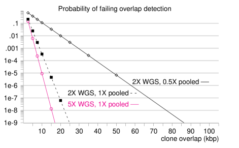
Figure 6. Clone overlap detection. The graph shows the probability of not detecting an overlap between two clones, as a function of the overlap size. The plots were calculated by a Monte-Carlo method using Theorem 2. All plots use $\vartheta=0.1$ for shotgun sequence overlap detection, and $\ell=500$ for shotgun sequence length.

5. BAC ordering

Our analyses so far have focused on detecting BAC overlaps via CAPS-MAP. This localized perspective was partly adopted to ease the theoretical analysis. In practice, mapping is performed based on a global clone-contig incidence matrix. The global approach exploits the dependencies in the collected data for increased accuracy. The algorithmic issues are very similar to those encountered in the context of STS-based physical mapping Gusfield. Define the mapping matrix $\mathbf{M}$ in which the rows correspond to the BACs, the columns correspond to the contigs, and $\mathbf{M}[i,j]=1$ if contig $j$ is linked to clone $i$, otherwise $\mathbf{M}[i,j]=0$. We want to find the true ordering of the rows and columns, defined by their physical locations on the genome. Assume for a moment that the matrix is completely error-free, i.e., all contigs are correctly assembled, and all contig-clone overlaps are detected. It is not hard to see that the row and column permutations corresponding to the correct ordering result in a matrix $\mathbf{M}^{\prime}$ that satisfies the consecutive ones property (C1P) in the rows and the columns: for every row $i$, there exist $a\leq b$ with $\mathbf{M}^{\prime}[i,j]=1$ if and only if $a\leq j\leq b$, and the same property holds for the columns. (A sufficient condition ensuring row-wise (or column-wise) C1P is that if the left endpoint of a contig (or a clone) precedes the left endpoint of another one, the same holds for their right endpoints.) Finding such permutations is a well-known problem C1P, and can be done in linear time. When the matrix is not error-free, one can use techniques introduced for STS-based physical mapping. In §6 we detail a method that relies on traveling salesperson tours.

6. CAPS-MAP simulation of Drosophila assembly

We tested the CAPS-MAP approach by simulating the assembly of the Drosophila melanogaster genome. One of the main goals of the simulated assembly was to predict the performance a hybrid approach combining WGS and CAPS sequences in a project that closely resembles the setup of the honey bee genome project’s (http://www.hgsc.bcm.tmc.edu/projects/honeybee/), currently pursued at the Human Genome Sequencing Center (HGSC) of Baylor College of Medicine.

Concatenating all the Drosophila genome sequence (Release 2.5, 112.6 million bases), 2880 BAC sequences were generated by randomly picking their locations and lengths. The mean BAC insert length was 150 kbp, and its standard deviation was 500 bp. The resulting random BAC library provides 3.6X coverage of the genome. BACs were arrayed by first partitioning them into 5 groups, and then using a two-array $24\times 24$ transversal design for each group. Every BAC was covered by 1.2X CAPS sequences: 0.4X per pool on the first array and 0.2X per pool on the second (reshuffled) array. In addition, WGS sequences were produced at 4X genome coverage. The shotgun sequences were generated using the program wgs-simulator (written by K. James Durbin), which mimics shotgun sequence collection realistically by relying on sequence quality files Phred.error produced in sequencing projects.

Shotgun sequences were assembled into contigs using the Atlas suite of genome assembly tools (http://www.hgsc.bcm.tmc.edu/downloads/software/atlas/) and Phrap (http://www.phrap.org/). A contig was mapped to a clone if it contained sequences from all four clone pools. Contigs that mapped to more than one BACs provided the evidence of BAC overlaps. BACs were grouped into maximal overlapping sets, or bactigs.

We compared the overlap graphs to assess CAPS-MAP overlap detection. The vertices of the overlap graphs are the BACs, and two BACs are connected if there is an overlap between them. The true overlap graph for the original BACs contains 2880 vertices, and 10992 edges in 66 graph components. The overlap graph calculated from the bactigs has 9193 edges in 110 components. Among its edges, 8527 (93%) are correct, and 2465 (22%) of the true overlaps are not discovered. The median length of detected overlaps is 87 kbp, and the median length of undetected overlaps is 42 kbp. There are 666 edges that correspond to no real overlaps. The vast majority of these “false positives” are instances when a long read contig links several BACs, which do not always overlap pairwise. All but two of the CAPS-MAP bactigs are true overlapping sets of BACs. CAPS-MAP links the assembled contigs to BACs correctly even in these two bactigs: the source of the error is the read contig assembly. Table 1 shows statistics on the bactig sizes and genome coverage.

Minimum bactig size	Genome covered	Number of BACs in bactigs
2	97.1%	2758
3	96.7%	2746
5	94.9%	2714
10	88.5%	2565
15	82.4%	2400
20	77.9%	2284
30	65.0%	1945
51	50.9%	1521
60	40.3%	1195

Table 1. Statistics for simulated Drosophila assembly. This table details the genome and BAC library coverage by bactig sizes. More than half of the genome is covered by bactigs with at least 51 BACs in them, defining the N50 statistic for the clone map.

BACs were ordered within each bactig. For every bactig, an overlap matrix $\mathbf{M}$ was calculated, in which the rows correspond to the bactig’s clones, the columns correspond to the contigs linked to at least one bactig clone, and $\mathbf{M}[i,j]=1$ if contig $j$ is linked to clone $i$, otherwise $\mathbf{M}[i,j]=0$. The following traveling salesperson (TSP) formulation is used to find the correct column permutation. We search for a tour in a graph, in which every vertex corresponds to a contig (and thus a column), with an additional vertex $u_{0}$. The weight of an edge between vertices $u$ and $u^{\prime}$, corresponding to contigs $j$ and $j^{\prime}$, is the number of rows in which they differ: $w(u,u^{\prime})=\sum_{i}\chi\Bigl{\{}\mathbf{M}[i,j]\neq\mathbf{M}[i,j^{\prime}]\Bigr{\}}$, where $\chi\{\cdot\}$ is the indicator function. The weight of an edge between $u$ and $u_{0}$ is the sum of ones in the column $j$ that corresponds to $u$: $w(u,u_{0})=\sum_{i}\mathbf{M}[i,j]$. Now, a Hamilton path with the minimum weight in this graph gives the best column permutation in the sense that it minimizes the number of gaps between blocks of ones within rows [Alizadeh, Karp, Newberg, and WeisserAlizadeh et al.1995]. The best row ordering could be found in an analogous manner, but we used a simpler method which worked better in practice. Clones are ordered relatively to the contig order by placing clone $B$ before $B^{\prime}$ if the first contig $B$ is linked to is before the first contig $B^{\prime}$ is linked to, or if their first contigs are identical but $B$ has its last contig before $B^{\prime}$.

We used the concorde program concorde to solve the TSP instances. The resulting row permutation is then further analyzed to find clones, for which the permutation arbitrarily enforces an order. Specifically, if consecutive rows of the permuted matrix $\mathbf{M}^{\prime}$ are identical, then the order of the corresponding clones is not resolved. Subsequently, we compared the TSP orders to the true orders, which is known since the BAC sequences are generated artificially. Figure 7 shows the outcome of the comparison for two bactigs. The TSP order is very close to the true order.

Figure 7. Correctness of BAC ordering in Drosophila simulation. The top (Loc) of each graph shows the relative physical location of each BAC, the middle (True) shows the correct BAC order, and the bottom (TSP) shows the TSP order, and the BAC identifiers. Identical BACs are connected in order to display the differences between the two permutations. The order of BACs at the bottom is not resolved when they are connected with a horizontal line. By resolving them optimally, bactig 23 produces the order of 72 BACs with 12 breakpoints and bactig 16 orders 50 BACs with 9 breakpoints. (Breakpoints are neighbors in the TSP order that are not neighbors in the true order.)

7. Discussion

The experimental expedience of shotgun sequencing has been essential for the success of genome-scale sequencing projects in the past decade. The power of the concept comes from the now established fact that the loss of information about read localization incurred by random subcloning can be largely recovered in the assembly step using sequence information. Clone pooling is similar in spirit to shotgun sequencing in that it introduces experimental expedience by dramatically reducing the number of subclone library preparations. The clone pooling step leads to a temporary loss of information about localization of shotgun sequences on individual BAC clones. We have demonstrated that sequence information can be used to successfully recover most of the information lost in pooling.

Our analyses presented here indicate the theoretical feasibility of the CAPS-MAP method and provide guidance for the design of genome-scale CAPS-MAP experiments. In particular, our analysis indicates that transversal pooling designs can accommodate high levels of clone redundancy and perform well even at low levels of shotgun sequence coverage of clone pools.

Practical biological and technical considerations may set a limit to the array size. In case of large genomes, the limitations may imply that the set of BACs is partitioned and that pooling is applied separately to individual subsets. This results in a lower clone redundancy within individual arrays and a larger number of pools. Our analysis allows for the partitioning of clones. It also allows for the possibility of including whole-genome shotgun sequence reads. It thus covers realistic and practical scenarios of the CAPSS and CAPS-MAP methods’ application.

Appendix

Here we expand our discussion on the probability of overlap detection in CAPS-MAP. In particular, we derive formulas that show the exponential decay of the probability of not detecting an overlap when the coverage $c_{2}$ is not too small. We start with the bound

(21) $$p_{\mathrm{nomap}}<\mathbb{E}\Bigl{[}\beta_{1}^{R}(2n)^{G+1}\Bigr{]}$$

Define

$$\mathcal{G}_{r}(z)={\mathbb{E}}\Bigl{[}z^{G}\Bigm{|}R\Bigr{]},$$

the probability generating function for the distribution of the number of gaps conditioned on the number of shotgun sequences. Define the events $A_{i}$ for $i=1,\dotsc,r-1$: $A_{i}$ denotes the event that the $i$-th sequence is followed by a gap, conditioned on the event $\{R=r\}$. For arbitrary $g$, and set of indexes $i_{1}<i_{2}<\dotsb<i_{g}$,

$$\mathbb{P}\Bigl{\{}A_{i_{1}}A_{i_{2}}\dotsm A_{i_{g}}\Bigr{\}}=(1-g\delta)_{+}^{r},$$

where $\delta=\frac{\sigma\ell}{\Theta L}$, and $(x)_{+}=\max\{0,x\}$ EG,WendlWaterston. Let

$$S_{0} =1$$

$$S_{g} =\sum_{i_{1}<\dotsb<i_{g}}\mathbb{P}\Bigl{\{}A_{i_{1}}A_{i_{2}}\dotsm A_{i_{g}}\Bigr{\}}=\binom{r-1}{g}(1-g\delta)_{+}^{r}.$$

Using inclusion-exclusion,

$${\mathbb{P}}\Bigl{\{}G=g\Bigm{|}R=r\Bigr{\}}=\sum_{j=g}^{r-1}\binom{j}{g}(-1)^{j-g}S_{j}.$$

Hence,

$$\mathcal{G}_{r}(z) =\sum_{g=0}^{r-1}z^{g}\sum_{j=g}^{r-1}\binom{j}{g}(-1)^{j-g}S_{j}$$

$$=\sum_{j=0}^{r-1}S_{j}\sum_{g=0}^{j}(-1)^{j-g}\binom{j}{g}z^{g}$$

$$=\sum_{j=0}^{r-1}S_{j}(z-1)^{j}.$$

Substituting the $S_{j}$ values:

(22) $$\mathcal{G}_{r}(z)=\sum_{j=0}^{r-1}\binom{r-1}{j}(1-j\delta)_{+}^{r}(z-1)^{j},$$

a result interesting on its own.

Returning to Equation (21), we have

(23) $$p_{\mathrm{nomap}}<\mathbb{E}\biggl{[}2n\beta_{1}^{R}\sum_{j=0}^{R-1}\binom{R-1}{j}(1-j\delta)_{+}^{R}(2n-1)^{j}\biggr{]},$$

where $R$ is a Poisson random variable with mean

$$\lambda=\frac{c_{2}\Theta L}{\ell}$$

For every $r\geq 0$, $(1-j\delta)_{+}^{r}\leq e^{-jr\delta}$, hence

$$\sum_{j=0}^{r-1}\binom{r-1}{j}(1-j\delta)_{+}^{r}(2n-1)^{j}\leq\Bigl{(}1+(2n-1)e^{-r\delta}\Bigr{)}^{r-1}.$$

Consequently, by Equation (23),

$$p_{\mathrm{nomap}}<\mathbb{E}\biggl{[}2n\beta_{1}^{R}\Bigl{(}1+(2n-1)e^{-R\delta}\Bigr{)}^{R-1}\biggr{]}.$$

Recall that the random value we take the expectation of is an upper bound on $p_{\mathrm{nomap}}(j_{0},\dotsc,j_{G})$, and thus if it is larger than one, it is useless. Let

$$f(r)=\min\Bigl{\{}1,2n\beta_{1}^{r}\Bigl{(}1+(2n-1)e^{-r\delta}\Bigr{)}^{r-1}\Bigr{\}}.$$

So we have in fact the bound

(24) $$p_{\mathrm{nomap}}<\mathbb{E}f(R).$$

In order to achieve exponential decay in the bound, we would like to have

$$\beta_{1}\Bigl{(}1+(2n-1)e^{-r_{0}\delta}\Bigr{)}<1$$

for some $r_{0}<\lambda$. Rearranging the inequality, we have

(25) $$(2n-1)\frac{n(a+w)+a}{(n-1)a}<e^{(2a+w)\sigma},$$

which is satisfied when $a$ and $w$ are not too small (see Figure 8).

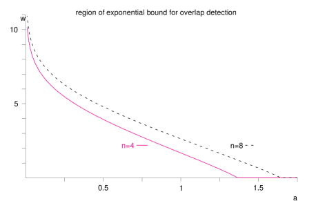
Figure 8. Values of the pooled shotgun coverage $a$ and WGS coverage $w$, for which the clone overlap detection bound applies, are above the graphs (see Equation (25))

.

There are several possible ways to exploit the fact that the exponential component of $f(r)$ becomes for $r$ less than the expected value $\lambda$. The main idea is that when evaluating $\mathbb{E}f(R)=\sum f(r)\mathbb{P}\{R=r\}$ in Equation (24), either the probability of $R=r$ is small, or the value of $f(r)$ is small. Let $0<k<\lambda$ be a threshold (that we specify later), and let $\alpha=k/\lambda$. To proceed with Equation (24), we condition on the event $\{R\leq\alpha\lambda\}$. We use the bound

(26) $$\mathbb{P}\{R\leq\alpha\lambda\}<\frac{e^{-\lambda(1-\alpha)^{2}/2}}{(1-\alpha)\sqrt{2\pi\alpha\lambda}},$$

which we prove here quickly. By definition,

$$\mathbb{P}\{R\leq\alpha\lambda\} \leq\sum_{r=0}^{k}\frac{{\lambda}^{r}}{r!}e^{-\lambda}<e^{-\lambda}\frac{{\lambda}^{k}}{k!}\sum_{r=0}^{k}\Bigl{(}\frac{k}{\lambda}\Bigr{)}^{r}$$

$$<e^{-\lambda}\frac{{\lambda}^{k}}{k!}(1-\alpha)^{-1}<e^{-\lambda(1-\alpha+\alpha\ln\alpha)}\frac{1}{(1-\alpha)\sqrt{2\pi\alpha\lambda}},$$

where we used a Stirling approximation: $k!>(k/e)^{k}/\sqrt{2\pi k}$. Using a Taylor series expansion,

$$1-\alpha+\alpha\ln\alpha=\frac{1}{2}(1-\alpha)^{2}+\frac{1}{6}(1-\alpha)^{3}+\frac{1}{12}(1-\alpha)^{4}\dotsc$$

and thus $1-\alpha+\alpha\ln\alpha>\frac{1}{2}(1-\alpha)^{2}$ for $0<\alpha<1$, and Equation (26) follows.

Now,

$$\mathbb{E}f(R) ={\mathbb{E}}\Bigl{[}f(R)\Bigm{|}R\leq\alpha\lambda\Bigr{]}\mathbb{P}\{R\leq\alpha\lambda\}+{\mathbb{E}}\Bigl{[}f(R)\Bigm{|}R>\alpha\lambda\Bigr{]}\mathbb{P}\{R>\alpha\lambda\}$$

$$\leq\mathbb{P}\{R\leq\alpha\lambda\}+{\mathbb{E}}\Bigl{[}f(R)\Bigm{|}R>\alpha\lambda\Bigr{]}$$

$$<\frac{e^{-\lambda(1-\alpha)^{2}/2}}{(1-\alpha)\sqrt{2\pi\alpha\lambda}}+\frac{2ne^{-\lambda}\sum_{r=0}^{\infty}\frac{\Bigl{(}\beta_{1}(1+(2n-1)e^{-\alpha\delta\lambda})\Bigr{)}^{r}}{r!}}{1+(2n-1)e^{-\alpha\delta\lambda}}$$

$$=\frac{\exp\Bigl{(}-\lambda(1-\alpha)^{2}/2\Bigr{)}}{(1-\alpha)\sqrt{2\pi\alpha\lambda}}+\frac{2n\exp\biggl{(}-\lambda\Bigl{(}1-\beta_{1}(1+(2n-1)e^{-\alpha c_{2}\sigma})\Bigr{)}\biggr{)}}{1+(2n-1)e^{-\alpha c_{2}\sigma}},$$

where we used $\delta\lambda=c_{2}\sigma$. Figure 9 shows values of $\alpha$ for different $a,w$ pairs that balance the exponents in the two terms.

Figure 9. Balanced $\alpha$ values for our exponential bound.

After choosing a balancing $\alpha$ value for a given $(a,w)$ pair, we obtain

$$\mathbb{E}f(R)<X_{1}\exp(-X_{2}\sigma L),$$

where $X_{1}$ and $X_{2}$ are constants that do not depend on $\sigma$. The bound becomes small ($<10^{-8}$) for larger $c_{2}$ values (e.g., $c_{2}=7$), but even then, it is not very tight. Based on simulation results, the tightness is lost with the inequality of Equation (21), and not in the following steps. For example, we evaluated the bounds of Equations (23) and (24) numerically. While they are fairly close to each other, and to the exponential bound using $\alpha$, they already bound the expected value of Equation (20) rather loosely in many cases. Furthermore, even for $(a,w)$ pairs for which we cannot establish exponential decay using the inequality of Equation (21), the overlap detection probability may get very close to one. For instance, a two-array design with $a=0.5$ and $w=2$ falls below the curve of Figure 8, yet can be employed efficiently in CAPS-MAP as shown in Figure 6. Therefore, we prefer using a Monte-Carlo evaluation of Equation (20) to predict the experimental performance of CAPS-MAP.

References

- [\citeauthoryearAlizadeh, Karp, Newberg, and WeisserAlizadeh et al.1995] Alizadeh, F., R. M. Karp, L. A. Newberg, and D. K. Weisser (1995). Physical mapping of chromosomes: a combinatorial problem in molecular biology. Algorithmica 13, 52–76.
-
[\citeauthoryearApplegate, Bixby, Chvátal, and
CookApplegate et al.1999]
Applegate, D., R. Bixby, V. Chvátal, and W. Cook (1999).
Concorde 99.12.15 release.
http://www.math.princeton.edu/tsp/concorde.html. - [\citeauthoryearArratia, Lander, Tavaré, and WatermanArratia et al.1991] Arratia, R., E. S. Lander, S. Tavaré, and M. S. Waterman (1991). Genomic mapping by anchoring random clones: A mathematical analysis. Genomics 11, 806–827.
- [\citeauthoryearBooth and LuekerBooth and Lueker1976] Booth, K. S. and G. S. Lueker (1976). Testing for the Consecutive Ones Property, interval graphs, and graph planarity using PQ-tree algorithms. Journal of Computer and System Sciences 13, 335–379.
- [\citeauthoryearCai, Chen, Gibbs, and BradleyCai et al.2001] Cai, W.-W., R. Chen, R. A. Gibbs, and A. Bradley (2001). A clone-array pooled strategy for sequencing large genomes. Genome Research 11, 1619–1623.
- [\citeauthoryearColbourn and DinitzColbourn and Dinitz1996] Colbourn, C. J. and J. H. Dinitz (Eds.) (1996). The CRC Handbook of Combinatorial Designs. Boca Raton: CRC Press.
- [\citeauthoryearCsűrös and MilosavljevicCsűrös and Milosavljevic2002] Csűrös, M. and A. Milosavljevic (2002). Pooled genomic indexing (PGI): mathematical analysis and experiment design. In Algorithms in Bioinformatics: Second International Workshop, Volume 2452 of LNCS, pp. 10–28. Berlin Heidelberg: Springer-Verlag.
- [\citeauthoryearDu and HwangDu and Hwang2000] Du, D.-Z. and F. K. Hwang (2000). Combinatorial Group Testing and Its Applications (2nd ed.). Singapore: World Scientific.
- [\citeauthoryearEwens and GrantEwens and Grant2001] Ewens, W. J. and G. R. Grant (2001). Statistical Methods in Bioinformatics: An Introduction. New York: Springer-Verlag.
- [\citeauthoryearEwing and GreenEwing and Green1998] Ewing, B. and P. Green (1998). Base-calling of automated sequencer traces using phred: II. error probabilities. Genome Research 8, 186–194.
- [\citeauthoryearGreenGreen2001] Green, E. D. (2001). Strategies for the systematic sequencing of complex genomes. Nature Reviews Genetics 2, 573–583.
- [\citeauthoryearGusfieldGusfield1997] Gusfield, D. (1997). Algorithms on Strings, Trees, and Sequences: Computer Science and Computational Biology. UK: Cambridge University Press.
- [\citeauthoryearIHGSCIHGSC2001] IHGSC (2001). Initial sequencing and analysis of the human genome. Nature 609(6822), 860–921.
- [\citeauthoryearLander and WatermanLander and Waterman1988] Lander, E. S. and M. S. Waterman (1988). Genomic mapping by fingerprinting random clones: a mathematical analysis. Genomics 2, 231–239.
- [\citeauthoryearMarra, Kucaba, Dietrich, Green, Brownstein, Wilson, McDonald, Hillier, McPherson, and WaterstonMarra et al.1997] Marra, M. A., T. A. Kucaba, N. L. Dietrich, E. D. Green, B. Brownstein, R. K. Wilson, K. M. McDonald, L. W. Hillier, J. D. McPherson, and R. H. Waterston (1997). High throughput fingerprint analysis of large-insert clones. Genome Research 7, 1072–1084.
- [\citeauthoryearWatermanWaterman1995] Waterman, M. S. (1995). Introduction to Computational Molecular Biology: Maps, Sequences and Genomes. Boca Raton: Chapman & Hall.
- [\citeauthoryearWeber and MyersWeber and Myers1997] Weber, J. L. and E. W. Myers (1997). Human whole-genome shotgun sequencing. Genome Research 7, 401–409.
- [\citeauthoryearWendl and WaterstonWendl and Waterston2002] Wendl, M. C. and R. H. Waterston (2002). Generalized gap model for bacterial artificial chromosome clone fingerprint mapping and shotgun sequencing. Genome Research 12, 1943–1949.