Modelling of SARS for Hong Kong

Abstract

A simplified susceptible-infected-recovered (SIR) epidemic model and a small-world model are applied to analyse the spread and control of Severe Acute Respiratory Syndrome (SARS) for Hong Kong in early 2003. From data available in mid April 2003, we predict that SARS would be controlled by June and nearly 1700 persons would be infected based on the SIR model. This is consistent with the known data. A simple way to evaluate the development and efficacy of control is described and shown to provide a useful measure for the future evolution of an epidemic. This may contribute to improve strategic response from the government. The evaluation process here is universal and therefore applicable to many similar homogeneous epidemic diseases within a fixed population. A novel model consisting of map systems involving the Small-World network principle is also described. We find that this model reproduces qualitative features of the random disease propagation observed in the true data. Unlike traditional deterministic models, scale-free phenomena are observed in the epidemic network. The numerical simulations provide theoretical support for current strategies and achieve more efficient control of some epidemic diseases, including SARS.

During 2003 SARS killed 916 and infected 8422 globallyWHO1 . In Hong Kong (HK), one of the most severely affected regions, 1755 individuals were infected and 299 diedHK1 . SARS is caused by a coronavirus, which is more dangerous and tenacious than the AIDS virus because of its strong ability to survive in moist air and considerable potential to infect through close personal contactLawrence1 ; Ksiazek1 ; Drosten1 ; Peiris1 . Unlike other well-known epidemic diseases, such as AIDS, SARS spreads quickly. Although significant, its mortality rate is, fortunately, relatively low (approximately 11%)WHO1 . Researchers have decoded the genome of SARS coronavirus and developed prompt diagnostic tests and some medicines, a vaccine is still far from being developed and widely usedMarra1 ; Rota1 ; Stadler1 . The danger of a recurrence of SARS remains.

Irrespective of pharmacological research, the epidemiology study of SARS will help to prevent possible spreading of similar future contagions. Generally, current epidemiological models are of two types. First, the well-known Susceptible-Infected-Recovered (SIR) model proposed in 1927Kermack1 ; Daley1 . Second, the concept of Small-World (SW) networksWatts1 . Arousing a new wave of epidemiological research, the SW model has made some progress recentlyDamian1 ; Holl1 ; Mode1 . Our work aims to model SARS data for HK. Practical advice for a better control are drawn from both the SIR and SW models. In particular, a generalized method to evaluate control of an epidemic is promoted here based on the SIR model with fixed population. Using this method, measuring the spread and control of various epidemics among different countries becomes simple. Quick action in the early stage is highlighted for both government and individuals to prevent rapid propagation.

I Susceptible-Infected-Recovered model

In the SIR model, the fixed population $N$ is divided into three distinct groups: Susceptible $S$, Infected $I$ and Removed $R$. Those at risk of the disease are susceptible, those that have it are infected and those that are either quarantined, dead, or have acquired immunity are removed. The following flow chart shows the basic procession of the SIR model Daley1 .

$$\begin{array}[]{ccccc}&rSI&&aI&\\ S&\rightarrow&I&\rightarrow&R\end{array}$$ (1)

Here $r$ and $a$ are the infection coefficient and removal rate, respectively. A discrete model was adapted by Gani from the original SIR model through the coarse-graining process and was applied to successfully predict outbreak of influenza epidemics in England and WalesGani1 ; Spicer1 .

$$S_{i+1} = S_{i}\left(1-rI_{i}\right)$$

$$I_{i+1} = \left[rS_{i}+\left(1-a\right)\right]I_{i}$$ (2)

$$R_{i+1} = R_{i}+aI_{i}$$

During the epidemic process, $N=S_{i}+I_{i}+R_{i}$ is fixed.

Initially, we examine the data for the first 15 days to estimate the parameters $r$ and $a$ of SARS for HK. The only data are new cases (removal $R$) announced everyday by HK Dept. of Health from March 12, 2003 followed by a revised version laterHK1 . To avoid inadvertently using future information we do not use the revised data at this stage. Population $N=7.3\times 10^{6}$; since $I+R\ll N$ it is reasonable to let $S_{i}=N$ in right hand side of (2). $I_{1}=1$ and $R_{1}=0$ is set as the initial condition. $I_{i}$ is replaced with $R_{i-1}$ whereas $I_{i}$ is uncertain. This assumption implies the incubation period is only one day, in spite of the fact that the true incubation period of the coronavirus is 2-7 daysRota1 . The parameters $r$ and $a$ are scanned for the best fit for the stage. For every $\left(r,a\right)$, a sequence of $R_{i+1}^{\prime}$ is obtained by numerical simulations. An Euclidean norm of $\sum_{i=1}^{15}\left(R_{i+1}-R_{i+1}^{\prime}\right)^{2}$, which indicates a distance between the true and simulated data, is applied to measure the fit. In Fig. 1 $\left(r,a\right)$ of the lowest point is the best fit parameters for this stage and this value is used for the following prediction. We get $r=2.05\times 10^{-7}$ and $a=1.444$. The method is applied to get parameters of $a$ and $r$ in Figs. 2 and 3.

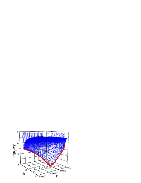
Figure 1: The quantity $\sum_{i=1}^{15}\left(R_{i+1}-R_{i+1}^{\prime}\right)^{2}$ vs. $r$ and $a$ is plotted as dots for the first 15 days SARS data for HK. The natural logarithm is applied. $R$ and $R^{\prime}$ are original and simulated data, respectively. The thick red curve shows the bottom of the sharp valley clearly. The lowest point of the valley is according to the best fit: $r=2.05\times 10^{-7}$ and $a=1.444$.

The prediction is available for the trend based on parameters $r$ and $a$ of this stage, the middle day (March 20, 2003) of the stage is applied as the first day and $\overline{R}=\frac{1}{15}\sum_{i=1}^{15}R_{i+1}$ is assumed as $\overline{I}$. A curve of squares is plotted in Fig. 2 for the first stage prediction. In the same way the best fit and prediction is applied for the next two stages and plotted in Fig. 2. The best fit is also processed weekly for detail discussion later.

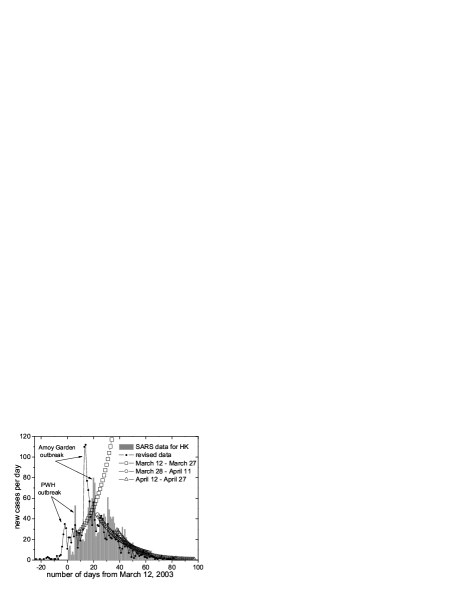
Figure 2: SARS data announced daily by the Hong Kong Dept. of Heath, the epidemic curve is plot as column graph. The curves of squares ($r=2.05\times 10^{-7}$ and $a=1.444$), circles ($r=1.55\times 10^{-7}$ and $a=1.172$) and triangles ($r=1.09\times 10^{-7}$ and $a=0.868$) are prediction for the 3 stages described in the text. Each stage has 15 days. The curve of black dots is for revised data.

The curves for prediction clearly shows the 3 stages in Fig. 2. The first stage (March 12 - 27, 2003) exhibits dangerous exponential growth. It shows that the extremely infectious SARS coronavirus spread quickly in the public with few protections during this early stage. More seriously, it leads to a higher infection peak although in this stage the averaged number of new cases $\overline{R}$ is below 30. This prediction gets confirmation in the second stage (March 28 - April 11, 2003). The peak characterized by the Amoy Garden outbreak comes earlier and higher. It indicates appearance of a new transmission mode that differs from intimate contact route observed in the first stage. We name the new transmission mode $explosive$ growth in the contrast to transmission in the first stage which we refer to as $burning$ growth. Outbreaks at Prince Wales Hospital (PWH) (where SARS patients received treatment) and Amoy Gardens (a high-density housing estate in Hong Kong) represent infections of $burning$ and $explosive$ modes in the full epidemic, respectively. The revised data provided by HK Dept. of Health in Fig. 2 present a clearer indication for these two transmission modes. The outbreak of PWH sent the clear message that intimate contacts with SARS patient led to infectionTomlinson1 . Detailed investigations of the propagation at Amoy Garden suggested that faulty of sewerage pipes allowed droplets containing the coronavirus to enter neighboring units vertically in the buildingRiley1 . Furthermore, poor ventilation of lifts and rat infestation where also suggested as possible modes of contamination Normile1 ; Ng1 ; Helen1 ; Donnelly1 . However, control measures bring the spread of the disease under control in the second stage. Contrary to the increasing trend in the first stage, the prediction curve of the 2nd stage (circle) declines. And it anticipates that new cases drop below 10 before the 60th day (May 10, 2003). Also on April 12, 2003 we predicted number of whole infection cases would reach 1700. Up to April 11, 2003 there were 32 deaths and 169 recoveriesHK1 . We calculated the mortality of SARS as the ratio of death to sum of both deathes and recoveries, and it was 15.9%. Therefore we predicted approximately 270 fatalities in total. In the third stage (April 12 - 27, 2003), triangle curve in Fig. 2 refines results and gives more accurate prediction. This stage predicts that new cases per day drops to 5 before the 62th day, May 12, 2003. The travel warning for HK was cancelled by WHO because HK had kept new cases below 5 for 10 days since May 15, 2003. And, finally, we predict that the total cases reaches 1730 and nearly 287 deaths (up to April 27, 2003 there were 668 recovered and 133, the mortality increased to 16.6%). These numbers are very close to the true dataHK1 . Precisely the method drawn from the SIR model has been verified for prediction for full epidemic. However, the accuracy is only possible by the first dividing the epidemic into separate ”stages”.

This problem of determining to what extent an epidemic is under control is of greater strategic significance. Information on the efficacy of epidemic control will help determine whether to apply more control policies or not, and balance cost and benefit from them. For each individual the same question will also inform the degree to which precautions are taken: i.e. wearing a surgical mask to prevent the spread (acquisition) of SARS. Obviously a way to estimate control level is required. Actually this is a difficult problem because of significant statistical fluctuations in the data. A quite simple method to evaluate control efficiency is discussed below.

In the SIR model (2), if $\Delta I=I_{i+1}-I_{i}\leq 0$ a disease is regards as being controlled as new cases will decrease. This inequality leads to a control criterion for some diseases in epidemiology research. Applying the approximation of $S_{i}=N$ we get a threshold $Nr\leq a$ from (2). We rescale $rN\rightarrow r$ ($r$ is called infection rate in place of infection coefficient now) and then get the threshold that is free from population $N$.

$$r\leq a$$ (3)

This indicates that the removal rate $a$ exceeds the infection rate $r$. In Fig. 3 the circles show the 3 stages evaluations with dash line of $r=a$. And the parameters $r$ and $a$ of SARS data for HK are estimated weekly as squares also in Fig. 3. The line of $r=a$ is regarded as the critical line since number of infected cases increases when $\left(r,a\right)$ passes through it from below. It is possible to apply the diagram of $r$ and $a$ to compare control level for different countries and areas even for different diseases. This provides organizations like WHO with a simple and standard method to supervise infection level of any disease. The limitation of the method comes from the assumptions of the SIR model. More accurate models may provide better estimate of epidemic state and future behaviours.

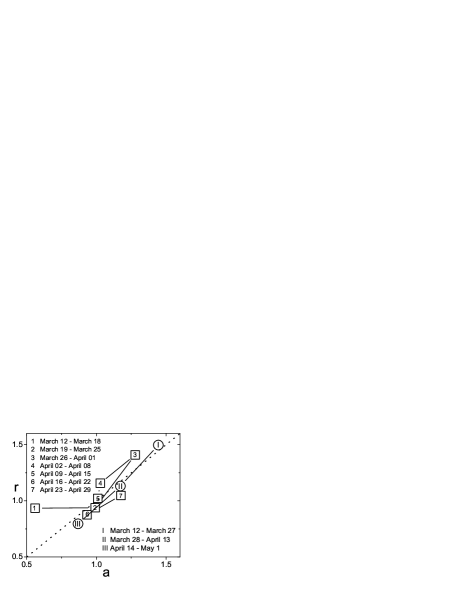
Figure 3: The best fit parameters estimated week by week from SARS data of HK are plotted as squares. The circles are for 3-stage analysis mentioned in Fig. 2. In this panel the line of dots $r=a$ is regarded as “alert line” or “critical line”. The parameters of $r$ and $a$ below it indicate that the epidemic is controlled, above the line indicates uncontrolled growth. The parameter $r$ is rescaled by $rN\rightarrow r$.

In summary, a discrete SIR model gives good predictions for epidemic of SARS for HK. Two distinct methods are described for the disease propagation dynamics. Particularly the $explosive$ mode is much more hazardous than the $burning$ mode. We have introduced a simple method to evaluate control levels. The method is generic and can be widely applied to various epidemiological data.

II The small-world model

Contrary to the long established SIR model, epidemiology research using Small-World (SW) network models is young and growing area. The concept of SW was imported from the study of social network into nature sciences in 1998Watts1 . However, it provides a novel insight for networks and arouses a lot of explorations in the brain, social networks and the Internet.Laughlin1 ; Albert1 ; Ebel1 ; Liljeros1 . Some SW networks also exhibit a scale-free (power law) distribution: a node in this network has probability $P(k)\sim k^{-\gamma}$ to connect $k$ nodes, $\gamma$ is one basic character for the systemAlbert1 ; Newman1 ; Ebel1 ; Liljeros1 . Most researches of “virus” spreading with the SW model, concern the propagation of computer viruses on the Internet, however, a few studies have been published relating to epidemiologyEbel1 ; Liljeros1 ; Strogatz1 ; Kuperman1 ; Huerta1 . The dynamics of SW models enriches our realization of epidemic and possibly provides better control policiesMiramontes1 . From the first SARS patient to the last one, an epidemic chain is embedded on the scale free SW network of social contacts. It is of great importance to discover the underlying structure of the epidemic network because a successful quarantine of all possible candidates for infection will lead to a rapid termination of the epidemic. In HK e-SARS, an electronic database to capture on-line and in real time clinical and administrative details of all SARS patients, provided invaluable quarantine information by tracing contactsHK1 ; Brower1 . Unfortunately a full epidemic network of SARS for HK is still unavailable. Because data representing the underlying network structure is currently not available, we have no choice other than numerical simulations. Therefore, our analysis of the SW model is largely theoretical. The only confirmation of our model we can offer is that the data appear to be realistic and exhibit the same features as the true epidemic data.

To simulate an epidemic chain, a simple model of social contacts is proposed . The model is established on a grid network weaved by $m$ parallel and $m$ vertical lines. Every node in the network represents a person. We set $m=2700$ with population $N=m^{2}=7.29\times 10^{6}$. All nodes are initiated with a value of 0 (named $good$ nodes). Every node has 2, 3 or 4 nearest neighbors as short range contacts for corner, edge and center, respectively. For every node there are two long range contacts with 2 other nodes randomly selected in the whole system everyday. These linkages model the social contact between individuals (i.e. social contacts that are sufficiently intimate to bring individuals at risk of spreading the disease). One random node of the system is set to 1 (called the $bad$ node), through its short and long range contacts, the value of the nodes linked with it turns into 1 according to probability of $p_{1}$ and $p_{2}$, respectively. An infection happens if a node changes its value from 0 to 1. This change is irreversible. During the full simulation process, the bad node is not removed from the whole system. We make this assumption because the number of deaths is small in comparision of the population, and there is no absolute quarantine—even the SARS patient in hospital can affect the medical workers. Moreover, the treatment period for SARS is relatively length, and during this time infected indviduals are highly infectious. To reflect the true variation in control strategy and individual behaviour, the control parameters $p_{1,2}$ ($0\leq p_{1,2}\leq 1$) vary with time.

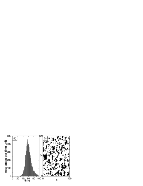
Figure 4: A plague is simulated in a geographical map with $100\times 100$ nodes with fixed infection probability $p_{1,2}=0.005$ which eventually leads to a full infection. a). The full epidemic curve of the simulated epidemic. b). While time is 45, the infection cases clusteringly scatter in the map. The infection happens in full scale map because of random connections. The clusters show effect from the nearest neighbour connections.

In same model it would be interesting to compare with the complete infection epidemic. A small system with $100\times 100$ nodes is chosen. A fixed probability $p_{1}=p_{2}=0.05$ leads to eventual infection of the entire population since all nodes are linked and the infected are not removed. The epidemic curve for this process is plotted in Fig. 4 a) and is typical of many plagues. In Fig. 4 b) various sizes of clusters with infected nodes (black dots) scatter over the geographical map. It contains all infection facts in first 45 days. Comparing to the true SARS infection distribution in HK only slight similarity is observed. The short and long range linkages give good infection dynamics as we expected. The epidemic chain is easily drawn by recording infection fact from the seed to last patient. However, during simulations there is a problem: for a $good$ node linked by more than one $bad$ nodes, which $bad$ node infects it? A widely accepted preferential attachment of rich-get-richer is a good answerAlbert1 ; Newman1 ; Watts2 . A linear preference function is applied here. With presence of both growth and preferential attachment, it is general to ask whether the chain is a scale-invariant SW network. We plot the distribution in Fig. 5 a) and b) in log-log and log-linear coordinates, respectively. The hollow circle is for the system with $100\times 100$ nodes. The scaling behaviour of it looks more like a piecewise linear (i.e. bilinear) in b) rather than a power law in a). To confirm this we tried a larger system with $1000\times 1000$ nodes and the same fixed $p_{1,2}$ in the rest curves in Figs. 5. The solid square curve is distribution of the whole epidemic network. The linear fit for the solid square gives a correlation coefficient $R$ of $-0.956$ in Fig. 5 a). In b) piecewise linear fits have $R$ of $-0.997$ and $-0.994$. These provide positive support for the original model. The ratio of the cases of first 30% and 1% of whole process for this bigger system are plotted as hollow triangle and solid circle curves in Figs. 5, respectively. The case of 1%, early stage of full infection epidemic, suggests a better fit for scale-free than the other cases since it has correlation coefficients $R$ of $-0.983$ and ratio $\gamma=-2.89$ for linear fit in a). For the solid circle curve piecewise linear fits give $R$ of $-0.995$ and $-0.977$ in Fig. 5 b). So, what scaling behaviour is true during full infection process? With absence of rigorous proof this problem is hard to answer correctly in simulations. We may only draw conclusions based on which simulations most closely matches the qualitative features of the observed data.

Figure 5: The scaling behaviour for a full infection epidemic network is plotted in log-log and log-linear coordinates in a) and b), respectively. The circle is for a full infection epidemic network simulated in a geographical map with $100\times 100$ nodes. The curves are for one with $1000\times 1000$ nodes. The curves of dots, triangles and squares are for the epidemic networks of 1% , 30% and 100% for full infection process. The two dash lines are piecewise linear fits for the full infection process with $1000\times 1000$ nodes. The ratio is $-0.31$ and $-0.07$ with $R=-0.997$ and $-0.994$, respectively. It clearly shows the curves of full epidemic has two piecewise linear parts in log-linear graph. In the early stage of a full infection, the scaling behaviour of 1% infected (dots) has a part which might be regards as a log-log linear. The ratio of it is $-2.89$ with $R=-0.983$. In other words, it has scale-free part with $\gamma=-2.89$.

Let’s return to the system with $2700\times 2700$ nodes for modelling SARS for HK. The probability $p_{1,2}$ is fitted to the true epidemic data. However, it is fruitless to obtain an exact coincidence between the simulated results and the true data as the model evolution is highly random (moreover this would result in overfitting). The control parameters $p_{1,2}$ (dots and dashes curves) and a simulated epidemic curve (black dots) with column diagram of SARS for HK is plotted in Figs. 6 a) and b), respectively. For the simulated data, the total number of cases is 1830 that has a 4.3% deviation from the true data of 1755. Contrary to the above full infection with fixed parameters, $p_{1,2}$ are believed to drop exponentially and lead to small part infection epidemic without quarantine or removal. In any case, the high probability of infection in the early stage is indicative of the critical ability of the SARS coronavirus to attack an individual without protection. If SARS returns, the same high initial infection level is likely to occur. The only hope to avoid a repeat of the SARS crisis of 2003 is to shorten the high infection stage by quick identification, wide protection and sufficient quarantining. In other words, the best time to eliminate possible epidemic is the moment that the first patient surfaces. Any delay may lead to a worsening crisis. The long range infections in the model and the world also imply an efficient mechanism to respond rapidly to any infectious disease is required to establish global control.

Figure 6: Control parameters and epidemic curve is plotted for the model with $2700\times 2700$ nodes. a) The short and long range linkages infection probability $p_{1,2}$ generally declines exponentially. b) The simulated epidemic curve (black dots) in the model is plotted with the original SARS data (grey column) for HK.

Figure 7: The distribution of infected nodes in simulations in two dimensional map. a). the whole geographical map; b). an amplified window of a cluster marked in circle of a).

Data on the geographical distribution of SARS cases in HK is much easier to collect than the full epidemic chain. Numerical simulations provide both simply. The full geographical map marked with all infected nodes (black dots) and an amplified window of a cluster is plotted in Figs. 7 a) and b), respectively. Similarity is expected and verified in cluster patterns of Figs. 4 b). The scaling behaviour of the epidemic chain is plotted in Figs. 8. The curve in log-log diagram exhibits a power-law coefficient of $\gamma=-3.55$ and gives the linear fit correlation coefficient $R=-0.989$. The piecewise linear fit for the log-linear case gives correlation coefficients $R$ of $-0.987$ and $-0.959$, respectively.

Figure 8: The scaling behaviour for the simulated epidemic network. In log-log coordinates, the scaling $P(k)\sim k^{-\gamma}$, $\gamma=-3.55$, where the linear fit exhibits a correlation coefficient $R=-0.989$.

For a SW network often few vertexes play more important roles than othersWatts2 . SARS super-spreaders found in HK, Singapore and China are consistent with thisRiley1 ; Leo1 . Data for the early spreading of SARS in SingaporeLeo1 show definite SW structure with a small number of nodes with a large number of links. The average number of links per node also shows a scale-free structure Leo1 , but the available data is extremely limited (the linear scaling can only be estimated from three observations).

This character is also verified in our model. The first few nodes have a high chance of infecting a large number of individuals. In Fig. 8, a single node has 40 links. Clearly the index node has many long range linkages. It has been suggested that travelling in crowded public places (train, hospital, even an elevator) without suitable precautions can cause an ordinary SARS patient to infect a significant number of others. Again, this is an indication that to increase an individual’s (especially a probable SARS patient’s) personal protection is key to rapidly control an epidemic. Actually, in our model, if duration of the early stage with high probability $p_{1,2}$ is reduced to less than 10, the infection scale decreases sharply.

An engrossing phenomenon is the points of inflection in curves in log-linear diagrams of Figs. 8 and Figs. 5 b). All are located near linkages number of 6-7. On average a nodes has about 6 contacts (2-4 short plus 2 long range) every day, although in whole process there is no limitation for linkages. For a growing random network, a general problem always exists among its scaling behaviour, preferential attachment and dynamics, even embedding a geographical mapCohen1 ; Warren1 ; Krapivsky1 ; Dorogovtsev1 ; Moore1 . More work is required to address this issue.

In conclusion a SW epidemic network is simulated to model SARS spreading in HK. A comparison of the simulations with full infection data is presented. Our discussion of the infection probability and occurrence of super spreaders lead to the obvious conclusion: rapid response of an individual and government is a key to eliminating an epidemic with limited impact and at minimal cost.

- (1) World Health Organization, Consensus Document on the Epidemiology of SARS, 17 Oct., 2003, http://www.who.int/csr/sars/en/WHOconsensus.pdf.
- (2) Report of the Severe Acute Respiratory Syndrome Expert Committee, 2 Oct., 2003, HK. http://www.sars-expertcom.gov.hk/english/reports/reports.html.
- (3) D. Lawrence, The Lancet 361, 1712 (2003).
- (4) T. G. Ksiazek, et al. New Engl. J. Med. 348, 1953 (2003).
- (5) C. Drosten, et al. New Engl. J. Med.; 348, 1967 (2003).
- (6) J. S. M. Peiris, et al. The Lancet 361, 1319 (2003).
- (7) M. A. Marra, et al. Science 300, 1399 (2003).
- (8) P. A. Rota, et al. Science 300, 1394 (2003).
- (9) K. Stadler, et al. Nature Rev. Microbio. 1, 209 (2003).
- (10) W. O. Kermack & A. G. McKerdrick, Proc. Roy. Soc. Lond. A 115, 700 (1927).
- (11) D. J. Daley, & J. Gani, Epidemic Modelling: An Introduction, (Cambridge Univ. press, Cambridge, 1999).
- (12) D. J. Watts, & S. H. Strogatz, Nature 393, 440 (1998).
- (13) H. Z. Damián & K. Marcelo, Physica A 309, 445 (2002).
- (14) J. Holl, et al. Nature 423, 605 (2003).
- (15) C. J. Mode & C. K. Sleeman, Math. Biosc. 156, 95 (1999).
- (16) J. Gani, J. Roy. Statist. Soc. Ser. A 141, 323 (1978).
- (17) C. C. Spicer, Brit. Med. Bull. 35, 23 (1979).
- (18) B. Tomlinson, & C. Cockram, The Lancet 361, 1486 (2003).
- (19) S. Riley, et al. Science 300, 1961 (2003).
- (20) D. Normile, Science 300, 714 (2003).
- (21) S. K C. Ng, The Lancet 362, 570 (2003).
- (22) C. A. Donnelly, et al. The Lancet 361, 1761 (2003).
- (23) P. Helen, Nature, 15 April (2003). http://www.nature.com/nsu/030414/030414-5.html.
- (24) S. B. Laughlin, & T. J. Sejnowski, Science 301, 1870 (2003).
- (25) R. Albert, & A.-L. Barabási, Rev. Mod. Phys. 74, 47 (2002).
- (26) M. Newman, Phys. Rev. E 64, 025102 (2001).
- (27) H. Ebel, et al. Phys. Rev. E 66, 035103 (2002).
- (28) F. Liljeros, et al. Nature 411, 907 (2001).
- (29) S. H. Strogatz, Nature 410, 268 (2001)
- (30) M. Kuperman, & G. Abramson, Phys. Rev. Lett. 86, 2909 (2001).
- (31) R. Huerta, & L. S. Tsimring, Phys. Rev. E 66, 056115 (2002).
- (32) O. Miramontes, & B. Luque, Physica D 168-169, 379 (2002).
- (33) V. Brower, EMBO Reports 4, 649 (2003).
- (34) R. Cohen, & S. Havlin, Phys. Rev. Lett. 90, 058701 (2003).
- (35) D. J. Watts, Small Worlds: The Dynamics of Networks between Order and Randomness, (Princeton Univ. press, Princeton, 1999).
- (36) Y. S. Leo, MMWR Weekly 52, 405 (2003).
- (37) C. P. Warren, et al. Phys. Rev. E 66, 056105 (2002).
- (38) P. L. Krapivsky, et al. Phys. Rev. Lett. 85, 4629 (2000).
- (39) S. N. Dorogovtsev, & J. F. F. Mendes, Phys. Rev. E 63, 056125 (2001).
- (40) C. Moore, & M. E. J. Newman, Phys. Rev. E 62, 7059 (2000).