Noise-driven transition to quasi-deterministic limit cycle dynamics in excitable systems

Abstract

The effect of small-amplitude noise on excitable systems with large time-scale separation is analyzed. It is found that small random perturbations of the fast excitatory variable result in the onset of a quasi-deterministic limit cycle behavior, absent without noise. The limit cycle is established at a critical value of the amplitude of the noise, and its period is nontrivially determined by the relationship between the noise amplitude and the time scale ratio. It is argued that this effect might provide a mechanism by which the function of biological systems operating in noisy environments can be robustly controlled by the level of the noise.

Understanding the effect of random perturbations in dynamical systems is a fundamental problem with a large number of applications in physical, chemical, and biological sciences. When these perturbations are small, noise-driven systems may often exhibit rare events which lead to switching-like dynamics on long time-scales Freidlin and Wentzell (1984). This behavior is well understood in systems obeying detailed balance, which is typical of systems close to thermal equilibrium (see, for example, Gardiner (1985)).

Systems far from equilibrium often fail to obey detailed balance. Even in the absence of noise, these systems are capable of having complex dynamical behaviors. One example of such a behavior is limit cycle oscillations. Another example is excitability: in excitable systems, small perturbations of the unique stable steady state decay, while sufficiently large perturbations lead to large-amplitude dynamical excursions before the system returns to the steady state (see, for example, Mikhailov (1990)). Excitable systems are very common in biology, with nerve cells being just one example (see, for example, Keener and Sneyd (1998)).

The purpose of this Letter is to show that under certain conditions small noise may transform the dynamics of an excitable system into a quasi-deterministic limit cycle, signifying a transition from excitable to oscillatory behavior under the action of the noise. This transition occurs at a critical value of the noise amplitude. Furthermore, the frequency and other parameters of the limit cycle are controlled by the amplitude of the noise, which distinguishes this mechanism from other mechanisms of noise-induced coherence (see, e.g., Gang et al. (1993); Pikovsky and Kurths (1997); Osipov and Ponizovskaya (2000)).

The key to our argument is the existence of a strong time scale separation in the system’s dynamics. In biology, this is typically the case: excitability often arises as a result of the competition of positive and negative feedbacks operating on different time-scales, with fast excitatory and slow recovery variables Keener and Sneyd (1998). In this situation it is possible to have an interplay between the slow deterministic time-scale of the recovery variable and the exponentially long time-scale associated with rare events induced by the noise. It is precisely this interplay that makes the considered effect possible.

Consider a general dynamical system

$$\dot{u} = f(u,v)+\sqrt{\varepsilon}\,\eta,$$ (1)

$$\dot{v} = \alpha g(u,v).$$ (2)

In the context of excitable systems, $u$ and $v$ (generally, vectors) will be sets of excitatory and recovery variables, respectively; $f$ and $g$ are the nonlinearities, $\alpha$ is the ratio of the time-scales, $\eta$ is some external noise perturbing the excitatory variables, and $\varepsilon\ll 1$ measures its amplitude. If $\alpha\ll 1$, there is a large time-scale separation in the deterministic part of the dynamics governed by $f$ and $g$, with $u$ and $v$ being the “fast” and the “slow” variables, respectively . That is, on the time-scale of order 1 the dynamics of $u$ is governed by (1) with $v$ frozen. Therefore, in the absence of the noise, the trajectory quickly approaches the slow manifold defined by the solutions of $f(u,v)=0$ for fixed $v$, and then proceeds on the time scale $\alpha^{-1}$ along this slow manifold and into the globally attracting equilibrium point.

With the introduction of the noise, the situation changes. Indeed, the trajectory may escape the slow manifold in the $u$ direction via a noise-activated process on the Arrhenius time-scale $\tau=\nu^{-1}\exp(\beta(v)/\varepsilon)\gg 1$, where $\beta(v)$ is some energy barrier to be crossed to initiate the escape and $\nu$ is some characteristic frequency Freidlin and Wentzell (1984). As a result, the system can perform a large excursion driven by the deterministic part of the dynamics, after which the trajectory can land again somewhere on the slow manifold. The dynamics can then proceed along the slow manifold until another escape event happens, and so on. This process may lead to a bona-fide limit cycle because of the following two ingredients. First, the interplay between the escape events and the motion along the slow manifold requires that their time-scales be comparable. But since the escape rate is a rapidly varying function of $v$, escape from the slow manifold will occur with overwhelming probability in the small vicinity of point $v=v_{\star}$ on this manifold, where $v_{\star}$ satisfies

$$\beta(v_{\star})=\varepsilon\log\alpha^{-1}.$$ (3)

Here we assumed that $\alpha,\varepsilon\to 0$ in a way that $\varepsilon\log\alpha^{-1}$ remains finite and neglected higher order terms. The next ingredient to obtain a limit cycle behavior is then a mechanism of reset. It requires that after a large excursion initiated from $v_{\star}$, the trajectory returns to the slow manifold to a point which leads again to $v_{\star}$ by the slow motion. Then the process will repeat itself indefinitely and the dynamics of the system will indeed be a limit cycle. Let us point out that the mechanism of escape at a fixed $v_{\star}$ is related to the phenomenon of stochastic resonance (for a review, see Gammaitoni et al. (1998)). Also note that the possibility of limit cycle behavior under the action of small noise in systems lacking such behavior in the absence of the noise was recently pointed out by Freidlin Freidlin (2001).

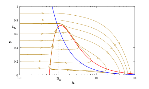
Figure 1: Deterministic flow generated by the nonlinearities from Eq. (4). Results of the numerical solution of Eqs. (1) and (2) in the $u-v$ plane for $A=0.7$ and $\alpha=0.01.$ Thick red and blue curves are the $u$- and $v$-nullclines, respectively.

To demonstrate the feasibility of the scenario above, we will consider the Brusselator Nicolis and Prigogine (1977). This is a prototypical model of a system far from equilibrium in which the nonlinearities take on the following form

$$f=1+u^{2}v-(1+A)u,\quad g=Au-u^{2}v.$$ (4)

Here $u$ and $v$ are scalars and $A$ is a control parameter. For simplicity we will assume that $\eta$ is external white Gaussian noise, with $\langle\eta(t)\eta(t^{\prime})\rangle=\delta(t-t^{\prime})$.

The Brusselator is an excitable system when $\alpha\ll 1$ and $A<1$. This can be seen from its phase portrait shown in Fig. 1. When $A<1$, the nullclines of Eqs. (1) and (2) intersect on the stable branch of the $u$-nullcline, so the flow is always into the unique equilibrium point

$$u_{0}=1,\qquad v_{0}=A.$$ (5)

Note that the slow manifold here is the rising part of the $u$-nullcline (see Fig. 1). It is also clear from the figure that sufficiently large increases in the $u$ variable away from equilibrium will result in large excursions.

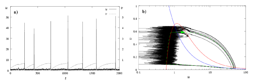
Figure 2: Numerical solution of the stochastic differential equation. The parameters are: $A=0.7,\alpha=0.01,\varepsilon=0.1$. (a) The time series with the quasi-periodic spike train. (b) The phase plane plot showing the quasi-deterministic limit cycle. Red and blue lines are the $u$- and $v$-nullclines, respectively. Solid green line is the predicted escape path and dashed green line is the excursion following the escape.

We performed numerical simulations of the stochastic differential equations given by Eqs. (1), (2), and (4). Fig. 2(a) shows the time series for one realization of the noise. This figure shows a train of large amplitude spikes in the excitatory variable. What is striking is that the spikes are occurring in an almost periodic fashion, with their amplitude and other characteristics being approximately the same. This can be better seen from the phase plane, Fig. 2(b). In fact, Fig. 2(b) strongly suggests a nearly limit cycle behavior in the $u$ and $v$ variables. To verify this, we computed the stationary probability distribution function (PDF) for this process (not shown). The PDF is found to be concentrated around a part of the slow manifold. One can also see a pronounced loop in the PDF for large values of $u$. Importantly, the PDF has a maximum at some value of $v=v_{\star}<v_{0}$. Let us point out that this result shows that our system lies beyond the region of applicability of the large deviations theory (if the latter were true, the PDF would be monotonically decreasing away from the equilibrium point Freidlin and Wentzell (1984)).

To further investigate the effect of the noise, we have analyzed the statistics of the interspike time intervals for different values of the noise amplitude $\varepsilon$. For the purpose of this analysis, we defined as a spike any excursion with an amplitude $u_{\mathrm{max}}\geq 10$. Fig. 3 shows the mean interspike distance $T$ and its standard deviation $\sigma_{T}$ obtained from the numerical solution of Eqs. (1), (2) and (4) for different value of the amplitude of the noise. Also, in the inset we show the ratio $\sigma_{T}/T$ as a function of $\varepsilon$, which characterizes the “signal-to-noise ratio” for the interspike distance.

First, observe that for very small $\varepsilon$ the spikes are exceedingly rare and have the character of a Poisson process (see the inset). They represent rare large-amplitude fluctuations away from the equilibrium point. Then, at some critical value of $\varepsilon\simeq 0.02$ the increase in the noise amplitude results in a rapid decrease in the interspike distance. Furthermore, the ratio $\sigma_{T}/T$ rapidly decreases and stays low in a broad range $0.05\lesssim\varepsilon\lesssim 0.5$, signifying high degree of signal coherence (see Fig. 2). Let us emphasize that in this range $T$ shows significant dependence on $\varepsilon$, while $\sigma_{T}$ does not (as seen from the errorbars). In other words, the noise amplitude really acts as a control parameter for the deterministic oscillatory behavior of the system. Finally, for larger noise amplitude, the spike train looses coherence again, since then the noise is no longer weak.

To explain these observations and corroborate the general scenario given above, let us consider the limit of strong time-scale separation. On the fast time-scale the value of $v$ is fixed, hence Eq. (1) describes the motion of a particle in the potential well of the form $V(u)=-\frac{1}{3}vu^{3}+\frac{1}{2}(1+A)u^{2}-u$. This is the classical escape problem of Kramers, for which the average escape time $\tau$ is given by the following formula Gardiner (1985)

$$\tau={2\pi\over\sqrt{(1+A)^{2}-4v}}\exp\left\{{[(1+A)^{2}-4v]^{3/2}\over 3v^{2}\varepsilon}\right\}.$$ (6)

From this equation, we obtain explicitly $\beta(v)={[(1+A)^{2}-4v]^{3/2}/3v^{2}}$. This $\beta(v)$ is inserted into Eq. (3), which fixes $v_{\star}$ as a function of $\alpha$ and $\varepsilon$.

Figure 3: Mean interspike distance $T$ and its standard deviation $\sigma_{T}$ (shown as errorbars) as a function of the noise amplitude. Inset: the plot of the ratio of the standard deviation to the mean. Except for the noise, the parameters are as in Fig. 2.

After the trajectory escapes the neighborhood of the stable nullcline at $v=v_{\star}$, it continues moving toward increasing values of $u$. At this point the effect of the noise becomes negligible. With the increase of $u$, the effective time-scale of $v$ decreases [see Eq. (2)], so when the system undergoes a large excursion, the time-scales of these two variables can no longer be separated. On the other hand, when $u\gg 1$ and $v\sim 1$, Eqs. (1) and (2) can be simplified by neglecting all the terms except $u^{2}v$. The resulting system of equations with the asymptotic boundary conditions $u(-\infty)=0$, $v(-\infty)=v_{\star}$ can be integrated to give $v=v_{\star}-\alpha u$ and $\dot{u}=u^{2}(v_{\star}-\alpha u)$. This equation can be solved exactly to give the transition layer for the rising part of the spike. It shows that in the spike $u$ rises to $u_{\mathrm{max}}=\alpha^{-1}v_{\star}\gg 1$ on the time-scale of $\alpha\ll 1$, while $v$ approaches zero asymptotically. This is then followed by the fall of the trajectory onto the $u$-nullcline with fixed (small) $v$ on the slower time scale of order 1, see Eq. (1) with $v=0$ (a more precise layer analysis of the solution can be performed Lubashevskii et al. ).

Following the excursion, on the slow time-scale the trajectory moves along the $u$-nullcline, starting at $v=0$ (asymptotically). After a little algebra we obtain for the slow motion:

$$\dot{v}={2\alpha(A-v)\over 1+A-2v+\sqrt{(1+A)^{2}-4v}}.$$ (7)

From Eq. (7), $\dot{v}>0$ for $0<v<v_{0}$, so the trajectory will reach the point $v=v_{\star}$ on the $u$-nullcline in time $T=T(v_{\star})$, which can be explicitly calculated by integrating Eq. (7). Upon reaching $v_{\star}$, the trajectory jumps off from the nullcline and returns onto the $u$-nullcline at the point where $v=0$, thus completing the loop [cf. Fig. 2(b)]. In summary, we obtain a limit cycle whose amplitude and period are asymptotically determined by the value of $v_{\star}$, which is in turn a function of $\alpha$ and $\varepsilon$.

Since the system spends most of the time on the slow manifold, asymptotically the period of the limit cycle will be equal to $T(v_{\star})$. This prediction can be compared with the mean interspike distance obtained from the simulations of Fig. 3. We found that the two are in qualitative agreement for $0.05\lesssim\varepsilon\lesssim 0.5$, but $T(v_{\star})$ consistently underestimates the observed value of $T$ by a factor of about 1.5. This is not unexpected, since the small parameter of the asymptotics is $1/\ln\alpha^{-1}$, which in practice is not very small. We verified that the accuracy increases with decrease of $\alpha$.

The above analysis also predicts the existence of a critical amplitude of the noise for the establishment of the limit cycle behavior. Indeed, the attainable values of $v$ on the $u$-nullcline lie in the interval $0<v<v_{0}$. Therefore, the solution of Eq. (3) may lie in this interval only if $\varepsilon>\varepsilon_{c}$, where

$$\varepsilon_{c}={(1-A)^{3}\over 3A^{2}\log\alpha^{-1}}.$$ (8)

No limit cycle behavior is possible when $\varepsilon<\varepsilon_{c}$. As $\varepsilon$ approaches $\varepsilon_{c}$ from above, we have $v_{\star}\to v_{0}$, and $T(v_{\star})\to\infty$. Therefore, for fixed deterministic part of the dynamics there is a transition to a limit cycle behavior at a critical value of the amplitude of the noise. We verified that the predicted value of $\varepsilon_{c}$ gives the correct order of magnitude for the onset of the oscillatory behavior.

Let us emphasize that the mechanism described above is robust: it does not require fine-tuning of the system’s parameters. This is in contrast with other mechanisms, by which noise can induce coherence (see, for example, Gang et al. (1993); Pikovsky and Kurths (1997); Osipov and Ponizovskaya (2000)). Those mechanisms require that in the absence of the noise the system is near the threshold between excitable and oscillatory behavior.

Now we discuss the potential implications of the observed phenomena. First of all, our results suggest that in systems with strong time-scale separation one should be careful in identifying the class of dynamical models for explaining the observations of oscillatory behaviors. Real systems are always noisy, and our analysis indicates that oscillatory behavior can be obtained in systems with intrinsically non-oscillatory dynamics. In particular, this may be relevant to the identification of cell types in model neural networks (see for example the discussions in Terman and Lee (1997); Vilar et al. (2002)). We note that the noise-induced transition similar to the one discussed in this Letter was recently observed in the numerical simulations of randomly forced Hodgkin-Huxley neuron Takahata et al. (2002).

Another possible implication has to do with coupled excitable systems. Our analysis indicates that in such systems the level of the noise, both extrinsic and intrinsic, may be used as an information carrier and transformed into (quasi-)deterministic signal. As a prototype, consider a system of all-to-all positively coupled excitable cells. Under the action of the noise of sufficiently small amplitude each cell will occasionally generate a spike. These spikes will have random phases, so their total input on each individual cell may average to a stationary random signal of low intensity. Now, if the noise level suddenly increases due to an external disturbance, the cells may switch to the noise-assisted oscillatory mode. This will further increase the effective noise amplitude, so that the oscillatory mode may persist even after the disturbance is removed. In colloquial terms, the system in a dormant state may wake up from the outside rattle.

In a similar way, our results may be applied to spatially distributed excitable media Mikhailov (1990). In these systems the analogue of the noise-activated event will be the formation of the radially-symmetric nucleus, leading to the consequent initiation of the radially-divergent wave Osipov and Muratov (1995); Muratov and Osipov (2001). In the wake of such a wave the system will undergo recovery. It is clear, then, that the system will be most recovered at the position where the wave was initiated. Hence, the new wave will be initiated again at the same spot, with the dynamics repeating periodically. This suggests that the well-known phenomenon of target pattern formation in two-dimensional excitable media Mikhailov (1990) might have an alternative interpretation in terms of noise-driven quasi-periodic wave generation.

C. B. M. is partially supported by NSF via grant DMS02-11864. E. V.-E. is partially supported by NSF via grants DMS01-01439, DMS02-09959 and DMS02-39625. W. E is partially supported by NSF via grant DMS01-30107.

References

- Freidlin and Wentzell (1984) M. I. Freidlin and A. D. Wentzell, Random Perturbations of Dynamical Systems (Springer-Verlag, New York, 1984).
- Gardiner (1985) C. W. Gardiner, Handbook of stochastic methods for physics, chemistry and the natural sciences (Springer-Verlag, Berlin, 1985).
- Mikhailov (1990) A. S. Mikhailov, Foundations of Synergetics (Springer-Verlag, Berlin, 1990).
- Keener and Sneyd (1998) J. Keener and J. Sneyd, Mathematical Physiology (Springer-Verlag, New York, 1998).
- Pikovsky and Kurths (1997) A. S. Pikovsky and J. Kurths, Phys. Rev. Lett. 78, 775 (1997).
- Gang et al. (1993) H. Gang, T. Ditzinger, C. Z. Ning, and H. Haken, Phys. Rev. Lett. 71, 807 (1993).
- Osipov and Ponizovskaya (2000) V. V. Osipov and E. V. Ponizovskaya, Phys. Rev. E 61, 4603 (2000).
- Gammaitoni et al. (1998) L. Gammaitoni, P. Hänggi, P. Jung, and F. Marchesoni, Rev. Mod. Phys. 70, 223 (1998).
- Freidlin (2001) M. I. Freidlin, J. Stat. Phys. 103, 283 (2001).
- Nicolis and Prigogine (1977) G. Nicolis and I. Prigogine, Self-Organization in Non-Equilibrium Systems (Wiley Interscience, New York, 1977).
- (11) I. A. Lubashevskii, C. B. Muratov, and V. V. Osipov, unpublished.
- Terman and Lee (1997) D. Terman and E. Lee, SIAM J. Appl. Math. 57, 252 (1997).
- Vilar et al. (2002) J. M. G. Vilar, H. Y. Kueh, N. Barkai, and S. Leibler, Proc. Natl. Acad. Sci. USA 99, 5988 (2002).
- Takahata et al. (2002) T. Takahata, S. Tanabe, and K. Pakdaman, Biol. Cybern. 86, 403 (2002).
- Muratov and Osipov (2001) C. B. Muratov and V. V. Osipov, Eur. Phys. J. B 22, 213 (2001).
- Osipov and Muratov (1995) V. V. Osipov and C. B. Muratov, Phys. Rev. Lett. 75, 338 (1995).