Material forces in the context of biotissue remodelling

Abstract

Remodelling of biological tissue, due to changes in microstructure, is treated in the continuum mechanical setting. Microstructural change is expressed as an evolution of the reference configuration. This evolution is expressed as a point-to-point map from the reference configuration to a remodelled configuration. A “preferred” change in configuration is considered in the form of a globally incompatible tangent map. This field could be experimentally determined, or specified from other insight. Issues of global compatibility and evolution equations for the resulting configurations are addressed. It is hypothesized that the tissue reaches local equilibrium with respect to changes in microstructure. A governing differential equation and boundary conditions are obtained for the microstructural changes by posing the problem in a variational setting. The Eshelby stress tensor, a separate configurational stress, and thermodynamic driving (material) forces arise in this formulation, which is recognized as describing a process of self-assembly. An example is presented to illustrate the theoretical framework.

1 Introduction

The development of biological tissue consists of distinct processes of growth, remodelling and morphogenesis—a classification suggested by Taber (1995). In our treatment of the problem, growth is defined as the addition or depletion of mass through processes of transport and reaction coupled with mechanics. As a result there is an evolution of the concentrations of the various species that make up the tissue. Nominally, these include the solid phase (cells and extra cellular matrix), the fluid phase (interstitial fluid), various amino acids, enzymes, nutrients, and byproducts of reactions between them. The stress and deformation state of the tissue also evolve due to mechanical loads, and the coupling between transport, reaction and mechanics.

Remodelling is the process of microstructural reconfiguration within the tissue. It can be viewed as an evolution of the reference configuration to a “remodelled” configuration. While it usually occurs simultaneously with growth, it is an independent process. For the purpose of conceptual clarity we will ignore growth in this paper, and focus upon a continuum mechanical treatment of remodelling.

The microstructural reconfiguration that underlies remodelling is a motion of material points in material space. An example of remodelling driven by stress is provided by the micrographs of Figure 1 from Calve et al. (2003).

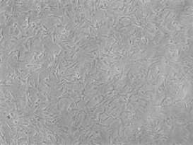
(a)

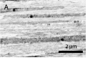
(b)

Figure 1: (a) Micrograph taken 3 days after plating of cells, shows a random distribution and orientation of tendon fibroblast cells in engineered tendon. (b) As growth occurs the cells organize into a more ordered microstructure seen in this micrograph taken about a month after plating of cells. The horizontal alignment of cells corresponds to the orientation of a uniaxial stress that was imposed externally on the growing tendon construct. The alignment of cells along the stress axis is evidence of remodelling due to stress in the engineered tendon during growth.

Remodelling also can be driven by the local density of the tissue’s solid or fluid phases, availability of various chemical factors, temperature, etc. We assume that it is possible (through experiments or other approaches) to define a phenomenological law that specifies this evolution. Since any conditions that could drive remodelling vary pointwise through the tissue, such a “preferred” remodelled state will, in general, be globally incompatible. However, in its final remodelled state, the tissue is virtually always free of such incompatibilities (see Figure 1). We therefore propose that a further, compatibilty-restoring material motion occurs, carrying material points to the remodelled configuration.

Taber and Humphrey (2001) and Ambrosi and Mollica (2002) have previously referred to remodelling. However, the treatments in these papers are based upon concentration (or density) changes in growing tissue and the mechanics—mainly internal stress—that is associated with them. By our definitions, these papers describe growth rather than remodelling. In a largely descriptive paper, Humphrey and Rajagopal (2002) have proposed the evolution of “natural configurations” that seems closest to our ideas. To our knowledge, however, no quantitative treatment exists paralleling the ideas of microstructural reconfiguration, material motion, material/configurational forces and their relation to remodelling, as described in the present paper.

2 Variational formulation: Material motion and material forces

Figure 2 depicts the kinematics associated with remodelling. The preferred remodelled state is given by a tangent map of material motion $\mbox{\boldmath$K$}^{\mathrm{r}}\colon\Omega_{0}\times[0,T]\mapsto\mathbb{GL}^{3}$, where $\mathbb{GL}^{3}$ is the space of $3\times 3$ matrices. The reference configuration is $\Omega_{0}\subset\mathbb{R}^{3}$. Our first assumption is that $\mbox{\boldmath$K$}^{\mathrm{r}}$ is given. Future communications will address the derivation of such an evolution law from our experiments (see Calve et al. (2003) for preliminary results). Since $\mbox{\boldmath$K$}^{\mathrm{r}}$ is generally incompatible (see Section 1), a further tangent map of material motion, $\mbox{\boldmath$K$}^{\mathrm{c}}\colon\Omega_{0}\times[0,T]\mapsto\mathbb{R}^{3}$, acts to render the tissue of interest, $\mathcal{B}$, compatible in its remodelled configuration, $\Omega^{\ast}_{t}$. The point-to-point map $\mbox{\boldmath$\kappa$}\colon\Omega_{0}\times[0,T]\mapsto\mathbb{R}^{3}$ carries material points from $\Omega_{0}$ to $\Omega^{\ast}_{t}\subset\mathbb{R}^{3}$, the remodelled configuration. It is a material motion, and its compatible tangent map, $\mbox{\boldmath$K$}=\partial\mbox{\boldmath$\kappa$}/\partial\mbox{\boldmath$X$}$ satisfies $\mbox{\boldmath$K$}=\mbox{\boldmath$K$}^{\mathrm{c}}\mbox{\boldmath$K$}^{\mathrm{r}}$. The placement of material points in $\Omega^{\ast}_{t}$ is $\mbox{\boldmath$X$}^{\ast}=\mbox{\boldmath$\kappa$}(\mbox{\boldmath$X$},t)$. Further deformation, brought about by the displacement, $\mbox{\boldmath$u$}^{\ast}$, carries material points from $\Omega^{\ast}_{t}$ to the spatial configuration $\Omega_{t}$. The deformation gradient is $\mbox{\boldmath$F$}^{\ast}={\bf 1}+\partial\mbox{\boldmath$u$}^{\ast}/\partial\mbox{\boldmath$X$}^{\ast}$. In this initial treatment we do not consider any further decompositions of $\mbox{\boldmath$F$}^{\ast}$. The overall motion of a point is $\mbox{\boldmath$\varphi$}(\mbox{\boldmath$X$},t)=\mbox{\boldmath$\kappa$}(\mbox{\boldmath$X$},t)+\mbox{\boldmath$u$}^{\ast}(\mbox{\boldmath$X$}^{\ast},t)\circ\mbox{\boldmath$\kappa$}(\mbox{\boldmath$X$},t)$, and the corresponding tangent map is $\mbox{\boldmath$F$}={\bf 1}+\partial\mbox{\boldmath$\varphi$}/\partial\mbox{\boldmath$X$}$. It admits the multiplicative decomposition $\mbox{\boldmath$F$}=\mbox{\boldmath$F$}^{\ast}\mbox{\boldmath$K$}^{\mathrm{c}}\mbox{\boldmath$K$}^{\mathrm{r}}$. To reiterate upon the foregoing distinction between the material motion and deformation components of the kinematics, we emphasize that $\mbox{\boldmath$u$}^{\ast}$ is a displacement, while $\kappa$ is a motion in material space. The corresponding tangent maps are $\mbox{\boldmath$F$}^{\ast}$ (a classical deformation gradient) and $K$ (a material motion gradient).

\psfrag{A}{\small$\Omega_{0}$}\psfrag{B}{\small$\Omega^{\ast}$}\psfrag{C}{\small$\Omega_{t}$}\psfrag{D}{\small$\mbox{\boldmath$\varphi$}$}\psfrag{G}{\small$\mbox{\boldmath$u$}^{\ast}$}\psfrag{E}{\small$\mbox{\boldmath$\kappa$}$}\includegraphics[width=284.52756pt]{remodel1.eps}

Figure 2: The kinematics of remodelling

2.1 A variational formulation

We consider the following energy functional:

$$\Pi[\mbox{\boldmath$u$}^{\ast},\mbox{\boldmath$\kappa$}] := \int\limits_{\Omega^{\ast}_{t}}\hat{\psi}^{\ast}(\mbox{\boldmath$F$}^{\ast},\mbox{\boldmath$K$}^{\mathrm{c}},\mbox{\boldmath$X$}^{\ast})\mathrm{d}V^{\ast}$$ (1)

$$-\int\limits_{\Omega^{\ast}_{t}}\mbox{\boldmath$f$}^{\ast}\cdot(\mbox{\boldmath$u$}^{\ast}+\mbox{\boldmath$\kappa$})\mathrm{d}V^{\ast}-\int\limits_{\partial\Omega^{\ast}_{t}}\bar{\mbox{\boldmath$t$}}^{\ast}\cdot(\mbox{\boldmath$u$}^{\ast}+\mbox{\boldmath$\kappa$})\mathrm{d}A^{\ast},$$

where $\psi^{\ast}=\hat{\psi}^{\ast}(\mbox{\boldmath$F$}^{\ast},\mbox{\boldmath$K$}^{\mathrm{c}},\mbox{\boldmath$X$}^{\ast})$ is the stored energy function. Observe that $\psi^{\ast}$ is assumed to depend upon the compatibility-restoring material motion, $\mbox{\boldmath$K$}^{\mathrm{c}}$, in addition to the usual dependence on $\mbox{\boldmath$F$}^{\ast}$. Furthermore, material heterogeneity is allowed. The body force per unit volume in $\Omega^{\ast}_{t}$ is $\mbox{\boldmath$f$}^{\ast}$, and the surface traction per unit area on $\partial\Omega^{\ast}_{t}$ is $\bar{\mbox{\boldmath$t$}}^{\ast}$. Since the total motion of a material point is $\mbox{\boldmath$\kappa$}+\mbox{\boldmath$u$}^{\ast}$, the potential energy of the external loads is as seen in the second and third terms.

Recall that the Euler-Lagrange equations obtained by imposing equilibrium with respect to $\mbox{\boldmath$u$}^{\ast}$ (stationarity of $\Pi$ with respect to variations in $\mbox{\boldmath$u$}^{\ast}$) represent the quasistatic balance of linear momentum in $\Omega^{\ast}_{t}$.

$$\frac{\mathrm{d}}{\mathrm{d}\varepsilon}\Pi[\mbox{\boldmath$u$}^{\ast}_{\varepsilon},\mbox{\boldmath$\kappa$}]\Big{|}_{\varepsilon=0}=0\;\mathrm{where}\;\mbox{\boldmath$u$}^{\ast}_{\varepsilon}=\mbox{\boldmath$u$}^{\ast}+\varepsilon\delta\mbox{\boldmath$u$}^{\ast}$$ (2)

$$\Longrightarrow\mathrm{Div}^{\ast}\mbox{\boldmath$P$}^{\ast}+\mbox{\boldmath$f$}^{\ast}=\hbox{\bf 0},\;\mathrm{in}\;\Omega^{\ast};\;\mbox{\boldmath$P$}^{\ast}\mbox{\boldmath$N$}^{\ast}=\bar{\mbox{\boldmath$t$}}^{\ast}\;\mathrm{on}\;\partial\Omega^{\ast};\;\mbox{\boldmath$P$}^{\ast}:=\frac{\partial\psi^{\ast}}{\partial\mbox{\boldmath$F$}^{\ast}},$$ (3)

Observe that the definition of $\mbox{\boldmath$P$}^{\ast}$ resembles the constitutive relation for the first Piola-Kirchhoff stress if $\Omega^{\ast}_{t}$ were the reference configuration.

A final assumption is that the tissue also reaches local equilibrium with respect to $\kappa$ (stationarity of $\Pi$ with respect to variations in $\kappa$). The variational statement is:

$$\frac{\mathrm{d}}{\mathrm{d}\varepsilon}\Pi[\mbox{\boldmath$u$}^{\ast},\mbox{\boldmath$\kappa$}_{\varepsilon}]\Big{|}_{\varepsilon=0}=0,\;\mathrm{where}\,\mbox{\boldmath$\kappa$}_{\varepsilon}=\mbox{\boldmath$\kappa$}+\varepsilon\delta\mbox{\boldmath$\kappa$},\;\mathrm{and}\,\mbox{\boldmath$\varphi$}\;\mathrm{is}\;\mathrm{fixed}.$$ (4)

The calculations are lengthy, but entirely standard, and yield the following Euler-Lagrange equations:

$$-\mathrm{Div}^{\ast}\left[\psi^{\ast}{\bf 1}-\mbox{\boldmath$F$}^{\ast^{\mathrm{T}}}\mbox{\boldmath$P$}^{\ast}+\frac{\partial\psi^{\ast}}{\partial\mbox{\boldmath$K$}^{\mathrm{c}}}\mbox{\boldmath$K$}^{\mathrm{c}^{\mathrm{T}}}\right]+\frac{\partial\psi^{\ast}}{\partial\mbox{\boldmath$X$}^{\ast}} = {\bf 0}\;\mathrm{in}\;\Omega^{\ast}$$ (5)

$$\left[\psi^{\ast}{\bf 1}-\mbox{\boldmath$F$}^{\ast^{\mathrm{T}}}\mbox{\boldmath$P$}^{\ast}+\frac{\partial\psi^{\ast}}{\partial\mbox{\boldmath$K$}^{\mathrm{c}}}\mbox{\boldmath$K$}^{\mathrm{c}^{\mathrm{T}}}\right]\mbox{\boldmath$N$}^{\ast} = {\bf 0}\;\mathrm{on}\;\partial\Omega^{\ast}.$$ (6)

Observe that the Eshelby stress $\psi^{\ast}{\bf 1}-\mbox{\boldmath$F$}^{\ast^{\mathrm{T}}}\mbox{\boldmath$P$}^{\ast}$ makes its appearance. Hereafter, it will be denoted ${\cal E}$. The term $\frac{\partial\psi^{\ast}}{\partial\mbox{\boldmath$K$}^{\mathrm{c}}}\mbox{\boldmath$K$}^{\mathrm{c}^{\mathrm{T}}}$ is a thermodynamic driving quantity giving the change in stored energy, $\psi^{\ast}$, corresponding to a change in configuration, $\mbox{\boldmath$K$}^{\mathrm{c}}$. It is stress-like in its physical dimensions and tensorial form, and we therefore refer to it as a configurational stress. Hereafter we will write $\mbox{\boldmath$\Sigma$}^{\ast}=\frac{\partial\psi^{\ast}}{\partial\mbox{\boldmath$K$}^{\mathrm{c}}}\mbox{\boldmath$K$}^{\mathrm{c}^{\mathrm{T}}}$.

Remark 1: A distinct class of variations can be considered than those in (4). Specifically, consider

$$\frac{\mathrm{d}}{\mathrm{d}\varepsilon}\Pi[\mbox{\boldmath$u$}^{\ast},\mbox{\boldmath$\kappa$}_{\varepsilon}]\Big{|}_{\varepsilon=0}=0,\;\mathrm{where}\,\mbox{\boldmath$\kappa$}_{\varepsilon}=\mbox{\boldmath$\kappa$}+\varepsilon\delta\mbox{\boldmath$\kappa$},\;\mathrm{and}\,\mbox{\boldmath$\varphi$}_{\varepsilon}=\mbox{\boldmath$X$}+\mbox{\boldmath$\kappa$}+\varepsilon\delta\mbox{\boldmath$\kappa$}+\mbox{\boldmath$u$}^{\ast},$$ (7)

which is distinct from (4) in that variations on the material motion result in variations on the final placement as well. In this case too, the Euler-Lagrange equations (5) and (6) are arrived at. This is an important property: The system of equations governing the evolution of the microstructural configuration must be independent of the particular class of variations considered.

2.2 Restrictions from the dissipation inequality

The dissipation inequality written per unit volume in the reference configuration takes the familiar form,

$$\mbox{\boldmath$\tau$}\colon(\dot{\mbox{\boldmath$F$}}\mbox{\boldmath$F$}^{-1})-\frac{\partial}{\partial t}\left(\mathrm{det}[\mbox{\boldmath$K$}]\psi^{\ast}\right)\geq 0,$$ (8)

where $\tau$ is the Kirchhoff stress defined in $\Omega_{t}$. Observe that $\mathrm{det}[\mbox{\boldmath$K$}]\psi^{\ast}$ is the stored energy per unit volume in $\Omega_{0}$. Using the multiplicative decomposition $\mbox{\boldmath$F$}=\mbox{\boldmath$F$}^{\ast}\mbox{\boldmath$K$}^{\mathrm{c}}\mbox{\boldmath$K$}^{\mathrm{r}}$, and the defining relation for the configurational stress $\mbox{\boldmath$\Sigma$}^{\ast}=\frac{\partial\psi^{\ast}}{\partial\mbox{\boldmath$K$}^{\mathrm{c}}}\mbox{\boldmath$K$}^{\mathrm{c}^{\mathrm{T}}}$, standard manipulations result in the following equivalent form:

$$\left(\mbox{\boldmath$\tau$}\mbox{\boldmath$F$}^{\ast^{-\mathrm{T}}}-\mathrm{det}[\mbox{\boldmath$K$}]\frac{\partial\psi^{\ast}}{\partial\mbox{\boldmath$F$}^{\ast}}\right)\dot{\mbox{\boldmath$F$}}^{\ast}-\mathrm{det}[\mbox{\boldmath$K$}]\left(\mbox{\boldmath${\cal E}$}+\mbox{\boldmath$\Sigma$}^{\ast}\right)\colon\left(\dot{\mbox{\boldmath$K$}}^{\mathrm{c}}{\mbox{\boldmath$K$}^{\mathrm{c}}}^{-1}\right)$$

$$-\mathrm{det}[\mbox{\boldmath$K$}]\mbox{\boldmath${\cal E}$}\colon\left(\mbox{\boldmath$K$}^{\mathrm{c}}\dot{\mbox{\boldmath$K$}}^{\mathrm{r}}\mbox{\boldmath$K$}^{-1}\right)-\mathrm{det}[\mbox{\boldmath$K$}]\frac{\partial\psi^{\ast}}{\partial\mbox{\boldmath$X$}^{\ast}}\cdot\dot{\mbox{\boldmath$\kappa$}}\geq 0.$$ (9)

Adopting the constitutive relation, $\mbox{\boldmath$\tau$}=\mathrm{det}[\mbox{\boldmath$K$}]\frac{\partial\psi^{\ast}}{\partial\mbox{\boldmath$F$}^{\ast}}\mbox{\boldmath$F$}^{\ast^{\mathrm{T}}}$ (this is consistent with the observation that $\mbox{\boldmath$P$}^{\ast}=\frac{\partial\psi^{\ast}}{\partial\mbox{\boldmath$F$}^{\ast}}$ is related to the first Piola-Kirchhoff stress with $\Omega^{\ast}_{t}$ as the reference configuration), results in the reduced dissipation inequality

$$-\mathrm{det}\mbox{\boldmath$K$}\left(\mbox{\boldmath${\cal E}$}+\mbox{\boldmath$\Sigma$}^{\ast}\right)\colon\left(\dot{\mbox{\boldmath$K$}}^{\mathrm{c}}{\mbox{\boldmath$K$}^{\mathrm{c}}}^{-1}\right)$$

$$-\mathrm{det}[\mbox{\boldmath$K$}]\mbox{\boldmath${\cal E}$}\colon\left(\mbox{\boldmath$K$}^{\mathrm{c}}\dot{\mbox{\boldmath$K$}}^{\mathrm{r}}\mbox{\boldmath$K$}^{-1}\right)-\mathrm{det}[\mbox{\boldmath$K$}]\frac{\partial\psi^{\ast}}{\partial\mbox{\boldmath$X$}^{\ast}}\cdot\dot{\mbox{\boldmath$\kappa$}}\geq 0,$$ (10)

which places restrictions on the evolution law for $\mbox{\boldmath$K$}^{\mathrm{r}}$, and on the functional dependencies $\hat{\psi}^{\ast}(\bullet,\mbox{\boldmath$K$}^{\mathrm{c}},\bullet)$ through $\mbox{\boldmath$\Sigma$}^{\ast}$, and $\hat{\psi}^{\ast}(\bullet,\bullet,\mbox{\boldmath$X$}^{\ast})$.

3 Remodelling of one-dimensional bars

In general, the examples of remodelling encountered in soft and hard biological tissue involve complex microstructural changes. Evolution laws for $\mbox{\boldmath$K$}^{\mathrm{r}}$ and the functional form, $\hat{\psi}^{\ast}(\bullet,\mbox{\boldmath$K$}^{\mathrm{c}},\bullet)$, to model these complexities are critical components for the successful application of the theoretical framework outlined in this paper. In future communications we will describe our experimental program to extract such constitutive information. However, the working of the formulation can be demonstrated by academic, but illuminating, examples. In the interest of brevity we restrict ourselves to a single example in this paper.

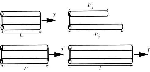
Figure 3: One-dimensional remodelling of bars.

Consider two parallel bars, that may represent adjacent strips of a long bone (Figure 3). We wish to consider a scenario in which each bar undergoes a preferred material motion to change its length from $L$ to $L_{i}^{\mathrm{r}},\;i=1,2$. In general, this configuration is incompatible as the bars can attain different lengths. If they are required to remain of the same length in the remodelled configuration, further material motion occurs, resulting in a length $L^{\ast}$ for each bar. This is the remodelled configuration, $\Omega^{\ast}_{t}$, in which the total material motion of each bar is $\kappa=L^{\ast}-L$. If the remodelling takes place under an external load, $T$, the bars each stretch to a final length $l$. The deformation is $u^{\ast}=l-L^{\ast}$. We examine the equations that govern the deformation and material motion by considering the following energy functional:

$$\Pi[u^{\ast},\kappa]=\frac{1}{2}k^{\ast}(\kappa+L-L^{\mathrm{r}}_{1})^{2}+\frac{1}{2}k^{\ast}(\kappa+L-L^{\mathrm{r}}_{2})^{2}+2\cdot\frac{1}{2}k{u^{\ast}}^{2}-T(u^{\ast}+\kappa),$$ (11)

where $k^{\ast}$ and $k$ are spring constants for the material motion- and stretch-dependent portions of the stored energy, respectively. These portions are assumed to be separable. The theory of Section 2 results in the following relations:

$$\frac{\partial\Pi}{\partial u^{\ast}}=0\quad\Rightarrow\;2ku^{\ast}=T,$$ (12)

$$\frac{\partial\Pi}{\partial\kappa}=0\quad\Rightarrow\;\mbox{\boldmath$\kappa$}=\frac{k}{k^{\ast}}u^{\ast}-\left(L-\frac{L^{\mathrm{r}}_{1}+L^{\mathrm{r}}_{2}}{2}\right).$$ (13)

In (12) the standard relation is seen for the stretch of a linear spring with effective stiffness $2k$. The more interesting result is (13). Observe that when $L=\frac{1}{2}(L_{1}^{\mathrm{r}}+L_{2}^{\mathrm{r}})$, material motion can occur, driven by stress, since $u^{\ast}=T/2k$ from (12). In this case remodelling can be incompatible if $L_{1}^{\mathrm{r}}\neq L_{2}^{\mathrm{r}}$. However, remodelling does not drive material motion, $\kappa$ in this case. Instead there is stress-driven remodelling as described in Section 1. On the other hand, in the absence of an external load, material motion is obtained when $L\neq\frac{1}{2}(L_{1}^{\mathrm{r}}+L_{2}^{\mathrm{r}})$. In this case the compatibility-restoring remodelling, motivated in Section 1 and described by the tangent map, $\mbox{\boldmath$K$}^{\mathrm{c}}$, also leads to overall material motion, $\kappa$.

4 Discussion and conclusion

This paper has presented a theoretical framework for remodelling in biological tissue, where this phenomenon is understood as an evolution of the microstructural configuration of the material. The assumption that the material attains local equilibrium with respect to the evolution of its microstructure results in Euler-Lagrange relations in the form of a governing partial differential equation and boundary conditions. The final form of the equations and the results themselves depend critically upon the specified constitutive relations for the preferred remodelled state of the material, and the dependence of the stored energy upon the compatibility-restoring component of remodelling. These are open problems, and will be addressed in future papers by our group. The following points are noteworthy at this stage of the development of the theory:

• This work does not deal with the approach to local equilibrium, which may take time on the order of days in biological tissue. Furthermore, the equilibrium state, being defined by the external loads, evolves upon perturbation of these conditions: Additional remodelling occurs in biological tissue when the load is altered.

• The energy functionals in (1) and (11) generalize to the Gibbs free energy of the body under constant loads and isothermal conditions. Further contributions that drive the process, such as chemistry or electrical stimuli, can be encompassed by the Gibbs energy. In such a setting the process we have described here would be termed a “self-assembly” in the realms of materials science or physics.

References

- Ambrosi and Mollica (2002) Ambrosi, D., Mollica, F., 2002. On the mechanics of a growing tumor. Int. J. Engr. Sci. 40, 1297–1316.
- Calve et al. (2003) Calve, S., Dennis, R., Kosnik, P., Baar, K., Grosh, K., Arruda, E., 2003. Engineering of functional tendon, submitted to Tissue Engineering.
- Humphrey and Rajagopal (2002) Humphrey, J. D., Rajagopal, 2002. A constrained mixture model for growth and remodeling of soft tissues. Math. Meth. Mod. App. Sci. 12 (3), 407–430.
- Taber (1995) Taber, L. A., 1995. Biomechanics of growth, remodelling and morphogenesis. Applied Mechanics Reviews 48, 487–545.