A continuum treatment of growth in biological tissue: The coupling of mass transport and mechanics

Abstract

Growth (and resorption) of biological tissue is formulated in the continuum setting. The treatment is macroscopic, rather than cellular or sub-cellular. Certain assumptions that are central to classical continuum mechanics are revisited, the theory is reformulated, and consequences for balance laws and constitutive relations are deduced. The treatment incorporates multiple species. Sources and fluxes of mass, and terms for momentum and energy transfer between species are introduced to enhance the classical balance laws. The transported species include: (i) a fluid phase, and (ii) the precursors and byproducts of the reactions that create and break down tissue. A notable feature is that the full extent of coupling between mass transport and mechanics emerges from the thermodynamics. Contributions to fluxes from the concentration gradient, chemical potential gradient, stress gradient, body force and inertia have not emerged in a unified fashion from previous formulations of the problem. The present work demonstrates these effects via a physically-consistent treatment. The presence of multiple, interacting species requires that the formulation be consistent with mixture theory. This requirement has far-reaching implications. A preliminary numerical example is included to demonstrate some aspects of the coupled formulation.

1 Background

Development of biological tissue, when described in the biomechanics literature, is generally broken down into the distinct processes of growth, remodelling and morphogenesis. Growth, or conversely, resorption, involves the addition or loss of mass. Remodelling results from a change in microstructure, which could manifest itself as an evolution of macroscopic quantities such as state of internal stress, stiffness or material symmetry. It also appears sometimes as fibrosis or hypertrophy. Morphogenesis involves both growth and remodelling, as well as more complex changes in form. A classical example of morphogenesis is the development of an embryo from a fertilized egg. These terms are based on the definitions developed by Taber (1995), and will be followed in this work. In the present communication we will focus exclusively on growth, its continuum formulation, and the implications that the process holds for the standard machinery of continuum mechanics. Remodelling is treated in an accompanying paper (Garikipati et al., 2003). The larger and more complex problem of morphogenesis will not be treated in this body of work.

The ideas here are applicable to soft (e.g., tendon, muscle) and hard (e.g., bone) tissue. In this paper, growth of biological tissue will be treated at a macroscopic scale. The continuum formulation (e.g., constitutive laws) at this scale may be motivated by cellular, sub-cellular or molecular processes. However, we will not explicitly model processes at this fine a scale. The formulation can be applied with a specific tissue e.g., muscle, as the body of interest. Our experiments, described separately, are on self-organizing tendon (Calve et al., 2003) and cardiac muscle constructs (Baar et al., 2003), engineered in vitro.

The principal notion to be borne in mind while developing a continuum formulation for growth is that one is presented with a system that is open with respect to mass. Scalar mass sources and sinks, and vectorial mass fluxes must be considered. A mass source was first introduced in the context of biological growth by Cowin and Hegedus (1976). The mass flux is a more recent addition of Epstein and Maugin (2000), who, however, did not elaborate on the specific nature of the transported species. Kuhl and Steinmann (2002) also incorporated the mass flux and specified a Fickean diffusive constitutive law for it. In their paper the diffusing species is the material of the tissue itself. The approach to mass transport that is followed in our paper is outlined in the next two paragraphs.

In order to be precise about the physiological relevance of our formulation, we have found it appropriate to adopt a different approach from the papers in the preceding paragraph in regard to mass transport. We do not consider mass transport of the material making up any tissue during growth. Instead, it is the nutrients, enzymes and amino acids necessary for growth of tissue, byproducts of metabolic reactions, and the tissue’s fluid phase (Swartz et al., 1999) that undergo diffusion in our treatment. There do exist certain physiological processes in which cells or the surrounding matrix migrate within a tissue. One such process is observed when leukocytes (white blood cells) such as neutrophils and monocytes are signalled to pass through a capillary wall and are induced, by specific chemical attractors, to migrate to a site of infection. This is the process of chemotaxis (Guyton and Hall, 1996; Widmaier et al., 2003). The migrant cells or matrix then participate in some form of cell proliferation or death. Fibroblasts also migrate within the extra cellular matrix during wound healing. A third example is the migration of stem cells to different locations during the embryonic development of an animal. These processes involve very short range diffusion, and can be treated by the approach described in this paper. We have chosen to focus upon homeostasis, defined by Widmaier et al. (2003) as “…a state of reasonably stable balance between the physiological variables…”. Since, to the best of our knowledge, processes of the type just described are not observed during homeostatic tissue growth, we will ignore transport of the solid phase of the tissue.

The processes of cell proliferation and death, hypertrophy and atrophy, are complex and involve several cascades of biochemical reactions. We will treat them in an elementary fashion, using source/sink terms that govern inter-conversion of species, and the mass fluxes that supply reactants and remove byproducts. The treatment will be mathematical; specific constituents will not be identified with any greater detail than to say that they are either the tissue’s solid phase, the interstitial fluid phase, precursors of the solid phase (these would include amino acids, nutrients and enzymes), or byproducts of reactions. We will return to explicitly incorporate biochemical and cellular processes within our description of mass transport in a subsequent paper.

Virtually all biological tissue consists of a solid and fluid phase and can be treated in the context of mixture theory (Truesdell and Toupin, 1960; Truesdell and Noll, 1965; Bedford and Drumheller, 1983). When growth is of interest, additional species (reactants and byproducts) must be considered as outlined above. The solid phase is an anisotropic composite that is inhomogeneous at microscopic and macroscopic scales. The fluid, being mostly water, may be modelled as incompressible, or compressible with a very large bulk modulus. This level of complexity will be maintained throughout our treatment. The use of mixture theory leads to difficulties associated with partitioning the boundary traction into portions corresponding to each species. Rajagopal and Wineman (1990), suggested a resolution to this problem that holds in the case of saturated media—a condition that is applicable to soft biological tissue. An alternative is to apply the theory of porous media that grew out of the classical work of Fick and Darcy in the 1800s (Terzaghi, 1943; de Boer, 2000). In this approach fluxes are introduced for each species. Since a species that diffuses must do so within some medium, one may think of the various constituents diffusing through the solid phase. This strategy has been adopted in the present work.

1.1 Recent work

In a simplification that avoided the complexity of mixture theory or porous media, Cowin and Hegedus (1976) accounted for the fluid phase via irreversible sources and fluxes of momentum, energy and entropy. This approach was also followed by Epstein and Maugin (2000) and Kuhl and Steinmann (2002). While the approach followed in the present paper, i.e. derivation of a mass balance law with mass source and flux, and postulating sources and fluxes for momentum, energy and entropy, has been attempted recently by Epstein and Maugin (2000), and Kuhl and Steinmann (2002), there are important differences between those works and our paper. Epstein and Maugin conclude that the mass flux vanishes unless the internal energy depends upon strain gradient terms (a second-order theory). This view ignores Fickean diffusion (where the flux is linearly dependent upon concentration of the relevant species). Our treatment also results in the dependence of mass flux upon strain gradient, but without the requirement of a strain gradient dependence of the internal energy. Instead, the dissipation inequality motivates a constitutive relation for the mass flux of each transported species. When properly formulated in a thermodynamic setting, the mass flux can be constrained to depend upon the strain/stress gradient and the gradient in concentration (mass per unit system volume) of the corresponding species. The latter term is the Fickean contribution to the mass flux. The form obtained is essentially identical to de Groot and Mazur (1984).

While modelling hard biological tissue, it is common to assume a Fickean flux, and a mass source that depends upon the strain energy density (Harrigan and Hamilton, 1993), and therefore upon the strain. This introduces coupling between mass transport and mechanics. One possible difficulty with this approach is that one could conceive of a mass source that satisfies other requirements, such as the dissipation inequality, but does not depend upon any mechanical quantities. Strain- or stress-mediated mass transport would then be absent in the boundary value problems solved with such a formulation.

The present paper is aimed at a complete treatment of mass transport, coupled with mechanics, for the growth problem. Initial sections (Sections 2–5) treat the balance of mass, balance of linear and angular momenta, the forms of the First and Second Laws for this problem, and kinematics of growth, respectively. The Clausius-Duhem inequality and its implications for constitutive relations are the subject of Section 6. Examples are provided as appropriate to illustrate the important results. A preliminary numerical example appears in Section 7. A discussion and conclusion are provided in Section 8.

2 Balance of mass for an open system

The body of interest, ${\mathcal{B}}$, occupies the open region $\Omega_{0}\subset\mathbb{R}^{3}$ in the reference configuration. Points in ${\mathcal{B}}$ are parameterized by their reference positions, $X$. The deformation of ${\mathcal{B}}$ is a point-to-point map, $\mbox{\boldmath$\varphi$}(\mbox{\boldmath$X$},t)\in\mathbb{R}^{3}$, of $\Omega_{0}$, carrying the point at $X$ to its current position $\mbox{\boldmath$x$}=\mbox{\boldmath$\varphi$}(\mbox{\boldmath$X$},t)$, at time $t\in[0,T]$. In its current configuration, ${\mathcal{B}}$ occupies the open region $\Omega_{t}=\mbox{\boldmath$\varphi$}_{t}(\Omega_{0}),\;\Omega_{t}\subset\mathbb{R}^{3}$ (see Figure 1). The tangent map of $\varphi$ is the deformation gradient $\mbox{\boldmath$F$}:=\partial\mbox{\boldmath$\varphi$}/\partial\mbox{\boldmath$X$}$.

\psfrag{BIGX}{\small$\mbox{\boldmath$X$}$}\psfrag{SMX}{\small$\mbox{\boldmath$x$}$}\psfrag{PI}{\small$\Pi^{\mathrm{\iota}}$}\psfrag{PPI}{\small$\pi^{\mathrm{\iota}}$}\psfrag{MN}{\small$\mbox{\boldmath$N$}\cdot\mbox{\boldmath$M$}^{\iota}$}\psfrag{MMN}{\small$\mbox{\boldmath$n$}\cdot\mbox{\boldmath$m$}^{\mathrm{\iota}}$}\psfrag{SN}{\small$\mbox{\boldmath$P$}\mbox{\boldmath$N$}$}\psfrag{SSN}{\small$\mbox{\boldmath$\sigma$}\mbox{\boldmath$n$}$}\psfrag{PHI}{\small$\mbox{\boldmath$\varphi$}$}\psfrag{WO}{\small$\Omega_{0}$}\psfrag{WT}{\small$\Omega_{t}$}\includegraphics[width=398.33858pt]{growth1.eps}

Figure 1: The continuum body with diffusing species and under stress.

The body consists of several species, of which the solid phase of the tissue is denoted $\mathrm{s}$, and the fluid phase is $\mathrm{f}$. The remaining species, $\alpha,\dots,\omega$, are precursors of the tissue or byproducts of its breakdown in chemical reactions. The index $\iota$ will be used to indicate an arbitrary species. (Where appropriate, we will use the term “system” to refer to the species collectively. Where the presence of several species is an unimportant fact, we will use the term “body”. ) The system is open with respect to mass. Species $\alpha,\dots,\omega$ have sources/sinks, $\Pi^{\alpha},\dots,\Pi^{\omega}$, and mass fluxes, $\mbox{\boldmath$M$}^{\alpha},\dots,\mbox{\boldmath$M$}^{\omega}$, respectively. The sources specify mass production rates per unit volume of the body in its reference configuration, $\Omega_{0}$. The fluxes specify mass flow rates per unit cross-sectional area in $\Omega_{0}$. Importantly, these flux vectors are defined relative to the solid phase. As discussed in Section 1, the solid tissue phase has only a mass source/sink associated with it, and no flux. The fluid tissue phase has only a mass flux, and no source/sink.

Since the solid phase, $\mathrm{s}$, does not undergo transport, its motion is specified entirely by $\mbox{\boldmath$\varphi$}(\mbox{\boldmath$X$},t)$. We describe the remaining species $\mathrm{f},\alpha,\dots,\omega$ as convecting with the solid phase and diffusing with respect to it. They therefore have a velocity relative to $\mathrm{s}$. Since the remaining species convect with $\mathrm{s}$, it implies a local homogenization of deformation. The modelling assumption is made that at each point, $X$, the individual phases undergo the same deformation.

We define concentrations of the species $\rho_{0}^{\iota}=\bar{\rho}_{0}^{\iota}f^{\iota}$ as masses per unit volume in $\Omega_{0}$. The intrinsic species density is $\bar{\rho}_{0}^{\iota}$, and $f^{\iota}$ is the volume fraction of $\iota$, for $\iota=\mathrm{s,f},\alpha,\dots,\omega$. In an experiment it is far easier to measure the concentration, $\rho_{0}^{\iota}$, rather than the intrinsic species density, $\bar{\rho}_{0}^{\iota}$. The concentrations also have the property $\sum\limits_{\iota}\rho_{0}^{\iota}=\rho_{0}$, the total material density of the tissue, with the sum being over all species $\mathrm{s,f},\alpha,\dots,\omega$. The concentrations, $\rho_{0}^{\iota}$, change as a result of mass transport and inter-conversion of species, implying that the total density in the reference configuration, $\rho_{0}$, changes with time. They are parameterized as $\rho_{0}^{\iota}(\mbox{\boldmath$X$},t)$.

2.1 Balance of mass in the reference configuration

Recall that $\Omega_{0}$ is a fixed volume. The statement of balance of mass of the solid phase of the tissue, written in integral form over $\Omega_{0}$, is

$$\frac{\mathrm{d}}{\mathrm{d}t}\int\limits_{\Omega_{0}}\rho_{0}^{\mathrm{s}}(\mbox{\boldmath$X$},t)\mathrm{d}V=\int\limits_{\Omega_{0}}\Pi^{\mathrm{s}}(\mbox{\boldmath$X$},t)\mathrm{d}V.$$ (1)

Since the solid phase of the tissue does not undergo mass transport, there is no associated flux. Localizing the result gives

$$\frac{\partial\rho_{0}^{\mathrm{s}}}{\partial t}=\Pi^{\mathrm{s}},$$ (2)

where the explicit dependence upon position and time has been suppressed.

The fluid phase of the tissue, $\mathrm{f}$, may be thought of as the interstitial or lymphatic fluid that perfuses the tissue. As explained above, we do not consider sources of fluid in the region of interest. The fluid therefore enters and leaves $\Omega_{0}$ as a flux, $\mbox{\boldmath$M$}^{\mathrm{f}}$. The balance of mass in integral form is

$$\frac{\mathrm{d}}{\mathrm{d}t}\int\limits_{\Omega_{0}}\rho_{0}^{\mathrm{f}}(\mbox{\boldmath$X$},t)\mathrm{d}V=-\int_{\partial\Omega_{0}}\mbox{\boldmath$M$}^{\mathrm{f}}(\mbox{\boldmath$X$},t)\cdot\mbox{\boldmath$N$}\mathrm{d}A,$$ (3)

where $N$ is the unit outward normal to the boundary, $\partial\Omega_{0}$. Applying the Divergence Theorem to the surface integral and localizing the result gives

$$\frac{\partial\rho_{0}^{\mathrm{f}}}{\partial t}=-\mbox{\boldmath$\nabla$}\cdot\mbox{\boldmath$M$}^{\mathrm{f}},$$ (4)

where $\mbox{\boldmath$\nabla$}(\bullet)$ is the gradient operator defined on $\Omega_{0}$, and $\mbox{\boldmath$\nabla$}\cdot(\bullet)$ denotes the divergence of a vector or tensor argument on $\Omega_{0}$.

For the precursor and byproduct species, $\iota=\alpha,\dots,\omega$, the balance of mass in integral form is

$$\frac{\mathrm{d}}{\mathrm{d}t}\int\limits_{\Omega_{0}}\rho_{0}^{\iota}(\mbox{\boldmath$X$},t)\mathrm{d}V=\int\limits_{\Omega_{0}}\Pi^{\iota}(\mbox{\boldmath$X$},t)\mathrm{d}V-\int_{\partial\Omega_{0}}\mbox{\boldmath$M$}^{\iota}(\mbox{\boldmath$X$},t)\cdot\mbox{\boldmath$N$}\mathrm{d}A.$$ (5)

In local form it is

$$\frac{\partial\rho_{0}^{\iota}}{\partial t}=\Pi^{\iota}-\mbox{\boldmath$\nabla$}\cdot\mbox{\boldmath$M$}^{\iota},\;\forall\,\iota=\alpha,\dots,\omega.$$ (6)

Of course, this last equation is the general form of mass balance for any species $\iota$, recalling that in particular, $\mbox{\boldmath$M$}^{\mathrm{s}}={\bf 0}$ and $\Pi^{\mathrm{f}}=0$. This form will be used in the development that follows.

The fluxes, $\mbox{\boldmath$M$}^{\iota},\;\forall\,\iota=\mathrm{f},\alpha,\dots,\omega$, represent mass transport of the fluid, of precursors to the reaction site, and of byproducts from sites of tissue breakdown. The sources, $\Pi^{\iota},\;\forall\iota=\mathrm{s},\alpha,\dots,\omega$, arise from inter-conversion of species. The sources/sinks in (2) and (6) are therefore related, as tissue and byproducts are formed by consuming precursors (amino acids and nutrients, for instance). To maintain a degree of simplicity in this initial exposition, we will restrict our description of tissue breakdown to the reverse of this reaction.

The sources, $\Pi^{\iota}$ for various species, satisfy a relation that is arrived as follows: Summing (6) over all species leads to the law of mass balance for the system,

$$\sum\limits_{\iota}\frac{\partial\rho_{0}^{\iota}}{\partial t}=\sum\limits_{\iota}\left(\Pi^{\iota}-\mbox{\boldmath$\nabla$}\cdot\mbox{\boldmath$M$}^{\iota}\right),$$ (7)

where the sum runs over all species, with $\Pi^{\mathrm{f}}=0$ and $\mbox{\boldmath$M$}^{\mathrm{s}}={\bf 0}$. Alternatively, in writing the mass balance equation for the system, the interconversion terms (sources/sinks) play no role, and only the fluxes at the boundaries need be accounted for. In integral form we have

$$\frac{\mathrm{d}}{\mathrm{d}t}\sum\limits_{\iota}\int\limits_{\Omega_{0}}\rho_{0}^{\iota}\mathrm{d}V=-\sum\limits_{\iota}\int\limits_{\partial\Omega_{0}}\mbox{\boldmath$M$}^{\iota}\cdot\mbox{\boldmath$N$}\mathrm{d}A.$$

Applying the Divergence Theorem and localizing leads to

$$\sum\limits_{\iota}\frac{\partial\rho_{0}^{\iota}}{\partial t}=\sum\limits_{\iota}(-\mbox{\boldmath$\nabla$}\mbox{\boldmath$M$}^{\iota}).$$ (8)

Comparing the equivalent forms (7) and (8) it emerges that the sources and sinks satisfy

$$\sum\limits_{\iota}\Pi^{\iota}=0,$$ (9)

a conclusion that is consistent with classical mixture theory (Truesdell and Noll, 1965). The section that follows contains an example in which the Law of Mass Action is invoked to describe a set of inter-related sources, $\Pi^{\iota}$.

2.1.1 Sources, sinks and stoichiometry: An example based upon the Law of Mass Action

The conversion of precursors to tissue and the reverse process of its breakdown are governed by a series of chemical reactions. The stoichiometry of these reactions varies in a limited range. Continuing in the simple vein adopted above, it is assumed that the formation of tissue and byproducts from precursors, and the breakdown of tissue, are governed by the forward and reverse directions of a single reaction:

$$\sum\limits_{\iota=\alpha}^{\omega}n_{\iota}[\iota]\longrightarrow[\mathrm{s}].$$ (10)

Here, $n_{\iota}$ is the (possibly fractional) number of moles of species $\iota$ in the reaction. For a tissue precursor, $n_{\iota}>0$, and for a byproduct, $n_{\iota}<0$. By the Law of Mass Action for this reaction, the rate of the forward reaction (number of moles of $\mathrm{s}$ produced per unit time, per unit volume in $\Omega_{0}$) is $k_{\mathrm{f}}\prod\limits_{\iota=\alpha}^{\omega}[\rho_{0}^{\iota}]^{n_{\iota}}$, where $\prod$ on the right hand-side denotes a product, not to be confused with the source, $\Pi$. The rate of the reverse reaction (number of moles of $\mathrm{s}$ consumed per unit time, per unit volume in $\Omega_{0}$) is $k_{\mathrm{r}}[\rho_{0}^{\mathrm{s}}]$, where $k_{f}$ and $k_{r}$ are the corresponding reaction rates. Assuming, for the purpose of this example, that the solid phase is a single compound, let the molecular weight of $\mathrm{s}$ be ${\mathcal{M}}_{\mathrm{s}}$. From the above arguments the source term for $\mathrm{s}$ is

$$\Pi^{\mathrm{s}}=\left(k_{\mathrm{f}}\prod\limits_{\iota=\alpha}^{\omega}[\rho_{0}^{\iota}]^{n_{\iota}}-k_{\mathrm{r}}[\rho_{0}^{\mathrm{s}}]\right){\mathcal{M}}_{\mathrm{s}},$$ (11)

Since the formation of one mole of $\mathrm{s}$ requires consumption of $n_{\iota}$ moles of $\iota$, we have

$$\Pi^{\iota}=-\left(k_{\mathrm{f}}\prod\limits_{\vartheta=\alpha}^{\omega}[\rho_{0}^{\vartheta}]^{n_{\vartheta}}-k_{\mathrm{r}}[\mathrm{s}]\right)n_{\iota}{\mathcal{M}}_{\iota},$$ (12)

where ${\mathcal{M}}_{\iota}$ is the molecular weight of species $\iota$. Since, due to conservation of mass, ${\mathcal{M}}_{\mathrm{s}}=\sum\limits_{\iota=\alpha}^{\omega}n^{\iota}{\mathcal{M}}_{\iota}$ the sources satisfy $\sum\limits_{\iota=\mathrm{s},\alpha}^{\omega}\Pi^{\iota}=0$.

2.2 Balance of mass in the current configuration

In the current configuration, $\Omega_{t}$, the concentration, source and mass flux of species $\iota$ are $\rho^{\iota}(\mbox{\boldmath$x$},t),\,\pi^{\iota}\mathrm{(}\mbox{\boldmath$x$},t)$, and $\mbox{\boldmath$m$}^{\iota}(\mbox{\boldmath$x$},t)$ respectively. The boundary is $\partial\Omega_{t}$, and has outward normal $n$ (Figure 1). Since the deformation, $\mbox{\boldmath$\varphi$}(\mbox{\boldmath$X$},t)$, is applied to the body (the system), standard arguments yield $\rho^{\iota}=\rho_{0}^{\iota}(\mathrm{det}\mbox{\boldmath$F$})^{-1}$, and $\pi^{\iota}=\Pi^{\iota}(\mathrm{det}\mbox{\boldmath$F$})^{-1}$. By Nanson’s formula, the normals satisfy $\mbox{\boldmath$n$}\mathrm{d}a=\mbox{\boldmath$F$}^{-\mathrm{T}}\mbox{\boldmath$N$}\mathrm{d}A$, where $\mathrm{d}A$ and $\mathrm{d}a$ are the area elements on the boundaries $\partial\Omega_{0}$ and $\partial\Omega_{t}$ respectively. The Piola transform then gives $\mbox{\boldmath$m$}^{\iota}=(\mathrm{det}\mbox{\boldmath$F$})^{-1}\mbox{\boldmath$F$}\mbox{\boldmath$M$}^{\iota}$.

The balance of mass in integral form for the solid tissue phase is

$$\frac{\mathrm{d}}{\mathrm{d}t}\int\limits_{\Omega_{t}}\rho^{\mathrm{s}}(\mbox{\boldmath$x$},t)\mathrm{d}v=\int\limits_{\Omega_{t}}\pi^{\mathrm{s}}(\mbox{\boldmath$x$},t)\mathrm{d}v.$$ (13)

Applying Reynolds’ Transport Theorem to the left hand-side, localizing the result and employing the product rule gives,

$$\frac{\partial\rho^{\mathrm{s}}}{\partial t}+\mbox{\boldmath$v$}\cdot\mbox{\boldmath$\nabla$}_{x}\rho^{\mathrm{s}}+\rho^{\mathrm{s}}\mbox{\boldmath$\nabla$}_{x}\cdot\mbox{\boldmath$v$}=\pi^{\mathrm{s}},$$

or,

$$\frac{\mathrm{d}\rho^{\mathrm{s}}}{\mathrm{d}t}=\pi^{\mathrm{s}}-\rho^{\mathrm{s}}\mbox{\boldmath$\nabla$}_{x}\cdot\mbox{\boldmath$v$},$$ (14)

where $\mbox{\boldmath$v$}(\mbox{\boldmath$x$},t)=\mbox{\boldmath$V$}(\mbox{\boldmath$X$},t)\circ\mbox{\boldmath$\varphi$}^{-1}(\mbox{\boldmath$x$},t)$ is the spatial velocity, $\mbox{\boldmath$\nabla$}_{x}(\bullet)$ is the spatial gradient operator, and $\mbox{\boldmath$\nabla$}_{x}\cdot(\bullet)$ is the spatial divergence. The time derivative on the left hand-side in (14) is the material time derivative, that may be written explicitly as $(\partial\rho^{\mathrm{s}}(\mbox{\boldmath$x$},t)/\partial t)_{X}$, implying that the reference position is held fixed.

For the fluid tissue phase, $\mathrm{f}$, the integral form is,

$$\frac{\mathrm{d}}{\mathrm{d}t}\int\limits_{\Omega_{t}}\rho^{\mathrm{f}}(\mbox{\boldmath$x$},t)\mathrm{d}v = -\int\limits_{\partial\Omega_{t}}\mbox{\boldmath$m$}^{\mathrm{f}}(\mbox{\boldmath$x$},t)\cdot\mbox{\boldmath$n$}\mathrm{d}a.$$ (15)

Invoking the Divergence Theorem in addition to the arguments used above for the solid phase now gives

$$\frac{\mathrm{d}\rho^{\mathrm{f}}}{\mathrm{d}t}=-\mbox{\boldmath$\nabla$}_{x}\cdot\mbox{\boldmath$m$}^{\mathrm{f}}-\rho^{\mathrm{f}}\mbox{\boldmath$\nabla$}_{x}\cdot\mbox{\boldmath$v$}.$$ (16)

Finally, for the precursor and byproduct species, $\iota=\alpha,\dots,\omega$, proceeding as above gives the local form in $\Omega_{t}$:

$$\frac{\mathrm{d}\rho^{\iota}}{\mathrm{d}t}=\pi^{\iota}-\mbox{\boldmath$\nabla$}_{x}\cdot\mbox{\boldmath$m$}^{\iota}-\rho^{\iota}\mbox{\boldmath$\nabla$}_{x}\cdot\mbox{\boldmath$v$},\;\forall\,\iota=\alpha,\dots,\omega.$$ (17)

3 Balance of linear and angular momenta

3.1 Balance of linear momentum

We first write the balance of linear momentum in the reference configuration, $\Omega_{0}$. The body, ${\mathcal{B}}$, is subject to surface traction, $T$, and body force per unit mass, $g$. The natural boundary condition then implies that $\mbox{\boldmath$T$}=\sum_{\iota}\mbox{\boldmath$P$}^{\iota}\mbox{\boldmath$N$}$ on $\partial\Omega_{0}$, where $\mbox{\boldmath$P$}^{\iota}$ is the partial first Piola-Kirchhoff stress tensor corresponding to species $\iota$, and the index runs over all species. Thus, $\mbox{\boldmath$P$}^{\iota}\mbox{\boldmath$N$}$ is the corresponding partial traction. The mass fluxes, $\mbox{\boldmath$M$}^{\iota},\;(\iota=\mathrm{f},\alpha,\dots,\omega)$, and mass sources, $\Pi^{\iota},\;(\iota=\mathrm{s},\alpha,\dots,\omega)$ make important contributions to the balance of linear momentum, as shown below.

The body undergoes deformation, $\mbox{\boldmath$\varphi$}(\mbox{\boldmath$X$},t)$, and has a material velocity field $\mbox{\boldmath$V$}(\mbox{\boldmath$X$},t)=\partial\mbox{\boldmath$\varphi$}(\mbox{\boldmath$X$},t)/\partial t$. In discussing momentum and energy, it proves convenient to define a material velocity of species $\iota$ relative to the solid phase as $\mbox{\boldmath$V$}^{\iota}=(1/\rho_{0}^{\iota})\mbox{\boldmath$F$}\mbox{\boldmath$M$}^{\iota}$. Recall (from Section 2) that the remaining species are described as deforming with the solid phase and diffusing relative to it. Therefore $F$ is common to all species. The spatial velocity corresponding to $\mbox{\boldmath$V$}^{\iota}$ is $\mbox{\boldmath$v$}^{\iota}=(1/\rho^{\iota})\mbox{\boldmath$m$}^{\iota}=\mbox{\boldmath$V$}^{\iota}$, by the Piola transform. Since fluxes are defined relative to the solid tissue phase, which does not diffuse, the total material velocity of the solid phase is $V$, and for each of the remaining species it is $\mbox{\boldmath$V$}+\mbox{\boldmath$V$}^{\iota}$, $\iota=\mathrm{f},\alpha,\dots,\omega$. Formally, we can write the material velocity as $\mbox{\boldmath$V$}+\mbox{\boldmath$V$}^{\iota}$, $\iota=\mathrm{s},\mathrm{f},\alpha,\dots,\omega$ with the understanding that $\mbox{\boldmath$V$}^{\mathrm{s}}={\bf 0}$. Likewise, $\Pi^{\mathrm{f}}=0$. This convention has been adopted in the remainder of the paper.

The balance of linear momentum of species $\iota$ written in integral form over $\Omega_{0}$ is,

$$\frac{\mathrm{d}}{\mathrm{d}t}\int\limits_{\Omega_{0}}\rho_{0}^{\iota}(\mbox{\boldmath$V$}+\mbox{\boldmath$V$}^{\iota})\mathrm{d}V = \int\limits_{\Omega_{0}}\rho^{\iota}_{0}\mbox{\boldmath$g$}\mathrm{d}V+\int\limits_{\Omega_{0}}\rho^{\iota}_{0}\mbox{\boldmath$q$}^{\iota}\mathrm{d}V+\int\limits_{\Omega_{0}}\Pi^{\iota}(\mbox{\boldmath$V$}+\mbox{\boldmath$V$}^{\iota})\mathrm{d}V$$ (18)

$$+\int\limits_{\partial\Omega_{0}}\mbox{\boldmath$P$}^{\iota}\mbox{\boldmath$N$}\mathrm{d}A-\int\limits_{\partial\Omega_{0}}(\mbox{\boldmath$V$}+\mbox{\boldmath$V$}^{\iota})\mbox{\boldmath$M$}^{\iota}\cdot\mbox{\boldmath$N$}\mathrm{d}A,$$

where $g$ is the body force per unit mass, and $\mbox{\boldmath$q$}^{\iota}$ is the force per unit mass exerted upon $\iota$ by the other species present. Attention is drawn to the fact that the mass source distributed through the volume, and the influx over the boundary affect the rate of change of momentum in (18). Summing over all species, the balance of linear momentum for the system is obtained:

$$\sum\limits_{\iota}\frac{\mathrm{d}}{\mathrm{d}t}\int\limits_{\Omega_{0}}\rho_{0}^{\iota}(\mbox{\boldmath$V$}+\mbox{\boldmath$V$}^{\iota})\mathrm{d}V = \sum\limits_{\iota}\int\limits_{\Omega_{0}}\rho^{\iota}_{0}\mbox{\boldmath$g$}\mathrm{d}V+\sum\limits_{\iota}\int\limits_{\Omega_{0}}\rho^{\iota}_{0}\mbox{\boldmath$q$}^{\iota}\mathrm{d}V$$ (19)

$$+\sum\limits_{\iota}\int\limits_{\Omega_{0}}\Pi^{\iota}(\mbox{\boldmath$V$}+\mbox{\boldmath$V$}^{\iota})\mathrm{d}V+\sum\limits_{\iota}\int\limits_{\partial\Omega_{0}}\mbox{\boldmath$P$}^{\iota}\mbox{\boldmath$N$}\mathrm{d}A$$

$$-\sum\limits_{\iota}\int\limits_{\partial\Omega_{0}}(\mbox{\boldmath$V$}+\mbox{\boldmath$V$}^{\iota})\mbox{\boldmath$M$}^{\iota}\cdot\mbox{\boldmath$N$}\mathrm{d}A,$$

The interaction forces, $\rho_{0}^{\iota}\mbox{\boldmath$q$}^{\iota}$, satisfy a relation with the mass sources, $\Pi^{\iota}$, that is elucidated by the following argument: The rate of change of momentum of the entire system is affected by external agents only, and is independent of internal interactions of any nature ($\mbox{\boldmath$q$}^{\iota}$ and $\Pi^{\iota}$). This observation leads to the following equivalent expression for the rate of change of linear momentum of the system:

$$\sum\limits_{\iota}\frac{\mathrm{d}}{\mathrm{d}t}\int\limits_{\Omega_{0}}\rho_{0}^{\iota}(\mbox{\boldmath$V$}+\mbox{\boldmath$V$}^{\iota})\mathrm{d}V = \int\limits_{\Omega_{0}}\rho_{0}\mbox{\boldmath$g$}\mathrm{d}V+\int\limits_{\partial\Omega_{0}}\mbox{\boldmath$P$}\mbox{\boldmath$N$}\mathrm{d}A$$ (20)

$$-\sum\limits_{\iota}\int\limits_{\partial\Omega_{0}}(\mbox{\boldmath$V$}+\mbox{\boldmath$V$}^{\iota})\mbox{\boldmath$M$}^{\iota}\cdot\mbox{\boldmath$N$}\mathrm{d}A.$$

Here, $\mbox{\boldmath$P$}=\sum\limits_{\iota}\mbox{\boldmath$P$}^{\iota}$ and $\rho_{0}=\sum\limits_{\iota}\rho_{0}^{\iota}$. Since both (19) and (20) represent the balance of linear momentum of the system, it follows that,

$$\sum\limits_{\iota}\int\limits_{\Omega_{0}}\rho^{\iota}_{0}\mbox{\boldmath$q$}^{\iota}\mathrm{d}V+\sum\limits_{\iota}\int\limits_{\Omega_{0}}\Pi^{\iota}(\mbox{\boldmath$V$}+\mbox{\boldmath$V$}^{\iota})\mathrm{d}V=0$$ (21)

Recalling the relation between the sources (9), and localizing leads to

$$\sum\limits_{\iota}\left(\rho^{\iota}_{0}\mbox{\boldmath$q$}^{\iota}+\Pi^{\iota}\mbox{\boldmath$V$}^{\iota}\right)=0,$$ (22)

a result that is also consistent with classical mixture theory (Truesdell and Noll, 1965).

Having established (22) we return to the balance of linear momentum for a single species (18) in order to simplify it. Writing $(\mbox{\boldmath$V$}+\mbox{\boldmath$V$}^{\iota})[\mbox{\boldmath$M$}^{\iota}\cdot\mbox{\boldmath$N$}]$ as $((\mbox{\boldmath$V$}+\mbox{\boldmath$V$}^{\iota})\otimes\mbox{\boldmath$M$}^{\iota})\mbox{\boldmath$N$}$, and using the Divergence Theorem,

$$\int\limits_{\Omega_{0}}\left(\frac{\partial\rho_{0}^{\iota}}{\partial t}\left(\mbox{\boldmath$V$}+\mbox{\boldmath$V$}^{\iota}\right)+\rho_{0}^{\iota}\frac{\partial}{\partial t}\left(\mbox{\boldmath$V$}+\mbox{\boldmath$V$}^{\iota}\right)\right)\mathrm{d}V=\int\limits_{\Omega_{0}}\rho^{\iota}_{0}\left(\mbox{\boldmath$g$}+\mbox{\boldmath$q$}^{\iota}\right)\mathrm{d}V\qquad$$

$$+\int\limits_{\Omega_{0}}\left(\Pi^{\iota}\left(\mbox{\boldmath$V$}+\mbox{\boldmath$V$}^{\iota}\right)+\mbox{\boldmath$\nabla$}\cdot\mbox{\boldmath$P$}^{\iota}\right)\mathrm{d}V$$

$$-\int\limits_{\Omega_{0}}\mbox{\boldmath$\nabla$}\cdot\left(\left(\mbox{\boldmath$V$}+\mbox{\boldmath$V$}^{\iota}\right)\otimes\mbox{\boldmath$M$}^{\iota}\right)\mathrm{d}V$$ (23)

Using the mass balance equation (6), and applying the product rule to the last term gives

$$\int\limits_{\Omega_{0}}\rho_{0}^{\iota}\frac{\partial}{\partial t}\left(\mbox{\boldmath$V$}+\mbox{\boldmath$V$}^{\iota}\right)\mathrm{d}V = \int\limits_{\Omega_{0}}\rho^{\iota}_{0}\left(\mbox{\boldmath$g$}+\mbox{\boldmath$q$}^{\iota}\right)\mathrm{d}V$$ (24)

$$+\int\limits_{\Omega_{0}}\left(\mbox{\boldmath$\nabla$}\cdot\mbox{\boldmath$P$}^{\iota}-\left(\mbox{\boldmath$\nabla$}\left(\mbox{\boldmath$V$}+\mbox{\boldmath$V$}^{\iota}\right)\right)\mbox{\boldmath$M$}^{\iota}\right)\mathrm{d}V$$

Localizing this result gives the balance of linear momentum for a single species in the reference configuration:

$$\rho_{0}^{\iota}\frac{\partial}{\partial t}\left(\mbox{\boldmath$V$}+\mbox{\boldmath$V$}^{\iota}\right)=\rho^{\iota}_{0}\left(\mbox{\boldmath$g$}+\mbox{\boldmath$q$}^{\iota}\right)+\mbox{\boldmath$\nabla$}\cdot\mbox{\boldmath$P$}^{\iota}-\left(\mbox{\boldmath$\nabla$}\left(\mbox{\boldmath$V$}+\mbox{\boldmath$V$}^{\iota}\right)\right)\mbox{\boldmath$M$}^{\iota}$$ (25)

The balance of linear momentum for a single species in the current configuration, $\Omega_{t}$, is obtained via similar arguments and the Reynolds Transport Theorem:

$$\rho^{\iota}\frac{\partial}{\partial t}\left(\mbox{\boldmath$v$}+\mbox{\boldmath$v$}^{\iota}\right) = \rho^{\iota}\left(\mbox{\boldmath$g$}+\mbox{\boldmath$q$}^{\iota}\right)+\mbox{\boldmath$\nabla$}_{x}\cdot\mbox{\boldmath$\sigma$}^{\iota}$$ (26)

$$-\left(\mbox{\boldmath$\nabla$}_{x}\left(\mbox{\boldmath$v$}+\mbox{\boldmath$v$}^{\iota}\right)\right)\mbox{\boldmath$m$}^{\iota}-\rho^{\iota}\left(\mbox{\boldmath$\nabla$}_{x}\left(\mbox{\boldmath$v$}+\mbox{\boldmath$v$}^{\iota}\right)\right)\mbox{\boldmath$v$},$$

where $\mbox{\boldmath$\sigma$}^{\iota}=(\mathrm{det}\mbox{\boldmath$F$})^{-1}\mbox{\boldmath$P$}^{\iota}\mbox{\boldmath$F$}^{\mathrm{T}}$ is the partial Cauchy stress of species $\iota$.

3.2 Angular Momentum

For the purely mechanical theory, balance of angular momentum implies that the Cauchy stress is symmetric: $\mbox{\boldmath$\sigma$}^{\iota}=\mbox{\boldmath$\sigma$}^{\iota^{\mathrm{T}}}$. We now re-examine this result in the presence of mass transport. At the outset one might expect a statement on the symmetry of some stress or stress-like quantity. We derive this result for any species, $\iota$, beginning with the integral form of balance of angular momentum written over $\Omega_{0}$.

$$\frac{\mathrm{d}}{\mathrm{d}t}\int\limits_{\Omega_{0}}\mbox{\boldmath$\varphi$}\times\rho^{\iota}_{0}(\mbox{\boldmath$V$}+\mbox{\boldmath$V$}^{\iota})\mathrm{d}V = \int\limits_{\Omega_{0}}\mbox{\boldmath$\varphi$}\times\left[\rho^{\iota}_{0}\left(\mbox{\boldmath$g$}+\mbox{\boldmath$q$}^{\iota}\right)+\Pi^{\iota}\left(\mbox{\boldmath$V$}+\mbox{\boldmath$V$}^{\iota}\right)\right]\mathrm{d}V$$ (27)

$$+\int\limits_{\partial\Omega_{0}}\mbox{\boldmath$\varphi$}\times\left(\mbox{\boldmath$P$}^{\iota}-\left(\mbox{\boldmath$V$}+\mbox{\boldmath$V$}^{\iota}\right)\otimes\mbox{\boldmath$M$}^{\iota}\right)\mbox{\boldmath$N$}\mathrm{d}A$$

Applying properties of the cross product, the Divergence Theorem and product rule gives

$$\int\limits_{\Omega_{0}}\mbox{\boldmath$V$}\times\rho^{\iota}_{0}\mbox{\boldmath$V$}^{\iota}+\mbox{\boldmath$\varphi$}\times\left(\frac{\partial\rho^{\iota}_{0}}{\partial t}\left(\mbox{\boldmath$V$}+\mbox{\boldmath$V$}^{\iota}\right)+\rho^{\iota}_{0}\frac{\partial}{\partial t}\left(\mbox{\boldmath$V$}+\mbox{\boldmath$V$}^{\iota}\right)\right)\mathrm{d}V=\qquad\quad$$

$$\int\limits_{\Omega_{0}}\mbox{\boldmath$\varphi$}\times\rho^{\iota}_{0}\left(\mbox{\boldmath$g$}+\mbox{\boldmath$q$}^{\iota}+\Pi^{\iota}\left(\mbox{\boldmath$V$}+\mbox{\boldmath$V$}^{\iota}\right)\right)\mathrm{d}V$$

$$+\int\limits_{\Omega_{0}}\left(\mbox{\boldmath$\varphi$}\times\mbox{\boldmath$\nabla$}\cdot\mbox{\boldmath$P$}^{\iota}-\mbox{\boldmath$\varphi$}\times\left(\mbox{\boldmath$\nabla$}\left(\mbox{\boldmath$V$}+\mbox{\boldmath$V$}^{\iota}\right)\mbox{\boldmath$M$}^{\iota}\right)\right)\mathrm{d}V$$

$$\int\limits_{\Omega_{0}}\left(-\mbox{\boldmath$\varphi$}\times\left(\mbox{\boldmath$V$}+\mbox{\boldmath$V$}^{\iota}\right)\mbox{\boldmath$\nabla$}\cdot\left(\mbox{\boldmath$M$}^{\iota}\right)\right)\mathrm{d}V$$

$$-\int\limits_{\Omega_{0}}\mbox{\boldmath$\epsilon$}\colon\left(\left(\mbox{\boldmath$P$}^{\iota}-\left(\mbox{\boldmath$V$}+\mbox{\boldmath$V$}^{\iota}\right)\otimes\mbox{\boldmath$M$}^{\iota}\right)\mbox{\boldmath$F$}^{\mathrm{T}}\right)\mathrm{d}V,$$ (28)

where $\epsilon$ is the permutation symbol, and $\mbox{\boldmath$\epsilon$}\colon\mbox{\boldmath$A$}$ is written as $\epsilon_{ijk}A_{jk}$ in indicial form, for any second-order tensor $A$. Using the mass balance equation (6), and balance of linear momentum (25), we have

$$\int\limits_{\Omega_{0}}\mbox{\boldmath$V$}\times\rho^{\iota}_{0}\mbox{\boldmath$V$}^{\iota}\mathrm{d}V=-\int\limits_{\Omega_{0}}\mbox{\boldmath$\epsilon$}\colon\left(\left(\mbox{\boldmath$P$}^{\iota}-\left(\mbox{\boldmath$V$}+\mbox{\boldmath$V$}^{\iota}\right)\otimes\underbrace{\mbox{\boldmath$M$}^{\iota}}_{\rho_{0}^{\iota}\mbox{\boldmath$F$}^{-1}\mbox{\boldmath$V$}^{\iota}}\right)\mbox{\boldmath$F$}^{\mathrm{T}}\right)\mathrm{d}V.$$

Recalling the relation of the permutation symbol to the cross product, and the indicated relation between $\mbox{\boldmath$M$}^{\iota}$ and $\mbox{\boldmath$V$}^{\iota}$ leads to

$${\bf 0}=-\int\limits_{\Omega_{0}}\mbox{\boldmath$\epsilon$}\colon\left(\left(\mbox{\boldmath$P$}^{\iota}-\mbox{\boldmath$V$}^{\iota}\otimes\rho_{0}^{\iota}\mbox{\boldmath$F$}^{-1}\mbox{\boldmath$V$}^{\iota}\right)\mbox{\boldmath$F$}^{\mathrm{T}}\right)\mathrm{d}V.$$ (29)

Localizing this result and again applying the properties of the permutation symbol we are led to the symmetry condition,

$$\left(\mbox{\boldmath$P$}^{\iota}-\mbox{\boldmath$V$}^{\iota}\otimes\rho^{\iota}_{0}\mbox{\boldmath$F$}^{-1}\mbox{\boldmath$V$}^{\iota}\right)\mbox{\boldmath$F$}^{\mathrm{T}}=\mbox{\boldmath$F$}\left(\mbox{\boldmath$P$}^{\iota}-\mbox{\boldmath$V$}^{\iota}\otimes\rho^{\iota}_{0}\mbox{\boldmath$F$}^{-1}\mbox{\boldmath$V$}^{\iota}\right)^{\mathrm{T}}.$$ (30)

But, $(\mbox{\boldmath$V$}^{\iota}\otimes\mbox{\boldmath$F$}^{-1}\mbox{\boldmath$V$}^{\iota})\mbox{\boldmath$F$}^{\mathrm{T}}=\mbox{\boldmath$V$}^{\iota}\otimes\mbox{\boldmath$V$}^{\iota}$. Thus, the symmetry $\mbox{\boldmath$P$}^{\iota}\mbox{\boldmath$F$}^{\mathrm{T}}=\mbox{\boldmath$F$}(\mbox{\boldmath$P$}^{\iota})^{\mathrm{T}}$ that results from conservation of angular momentum for the purely mechanical theory, is retained in this case. The partial Cauchy stresses are therefore symmetric: $\mbox{\boldmath$\sigma$}^{\iota}=\mbox{\boldmath$\sigma$}^{\iota^{\mathrm{T}}}$. This is in contrast with the non-symmetric Cauchy stress arrived at by Epstein and Maugin (2000). The origin of this difference lies in the fact that these authors use a single species with $\mbox{\boldmath$V$}=\partial\mbox{\boldmath$\varphi$}/\partial t$ as the material velocity, rather than multiple species with material velocities $\mbox{\boldmath$V$}+\mbox{\boldmath$V$}^{\iota}$.

4 Balance of energy and the entropy inequality

4.1 Balance of energy

Since mass is undergoing transport with respect to ${\mathcal{B}}$, and inter-conversion between species $\iota=\mathrm{s},\alpha,\dots,\omega$, it is appropriate to work with energy and energy-like quantities per unit mass. In addition to the terms introduced in previous sections, the internal energy per unit mass of species $\iota$ is denoted $e^{\iota}$; the heat supply to species $\iota$ per unit mass of that species is $r^{\iota}$; and the partial heat flux vector of $\iota$ is $\mbox{\boldmath$Q$}^{\iota}$, defined on $\Omega_{0}$. An interaction energy appears between species: The energy transferred to $\iota$ by all other species is $\tilde{e}^{\iota}$, per unit mass of $\iota$. In the arguments to follow in this section we will use the fluxes $\mbox{\boldmath$M$}^{\iota}$ and the associated velocities, $\mbox{\boldmath$V$}^{\iota}$. Working in $\Omega_{0}$, we relate the rate of change of internal and kinetic energies of species $\iota$ to the work done on $\iota$ by mechanical loads, processes of mass production and transport, heating and energy transfer:

$$\frac{\mathrm{d}}{\mathrm{d}t}\int\limits_{\Omega_{0}}\rho_{0}^{\iota}\left(e^{\iota}+\frac{1}{2}\|\mbox{\boldmath$V$}+\mbox{\boldmath$V$}^{\iota}\|^{2}\right)\mathrm{d}V=\int\limits_{\Omega_{0}}\left(\rho_{0}^{\iota}\mbox{\boldmath$g$}\cdot\left(\mbox{\boldmath$V$}+\mbox{\boldmath$V$}^{\iota}\right)+\rho_{0}^{\iota}r^{\iota}\right)\mathrm{d}V\qquad$$

$$+\int\limits_{\Omega_{0}}\rho_{0}^{\iota}\mbox{\boldmath$q$}^{\iota}\cdot(\mbox{\boldmath$V$}+\mbox{\boldmath$V$}^{\iota})\mathrm{d}V$$

$$+\int\limits_{\Omega_{0}}\left(\Pi^{\iota}\left(e^{\iota}+\frac{1}{2}\|\mbox{\boldmath$V$}+\mbox{\boldmath$V$}^{\iota}\|^{2}\right)+\rho^{\iota}_{0}\tilde{e}^{\iota}\right)\mathrm{d}V$$

$$+\int\limits_{\partial\Omega_{0}}\left(\left(\mbox{\boldmath$V$}+\mbox{\boldmath$V$}^{\iota}\right)\cdot\mbox{\boldmath$P$}^{\iota}-\mbox{\boldmath$M$}^{\iota}\left(e^{\iota}+\frac{1}{2}\|\mbox{\boldmath$V$}+\mbox{\boldmath$V$}^{\iota}\|^{2}\right)-\mbox{\boldmath$Q$}^{\iota}\right)\cdot\mbox{\boldmath$N$}\mathrm{d}A.$$ (31)

Summing over all species, the rate of change of energy of the system is,

$$\sum\limits_{\iota}\frac{\mathrm{d}}{\mathrm{d}t}\int\limits_{\Omega_{0}}\rho_{0}^{\iota}\left(e^{\iota}+\frac{1}{2}\|\mbox{\boldmath$V$}+\mbox{\boldmath$V$}^{\iota}\|^{2}\right)\mathrm{d}V=\sum\limits_{\iota}\int\limits_{\Omega_{0}}\left(\rho_{0}^{\iota}\mbox{\boldmath$g$}\cdot\left(\mbox{\boldmath$V$}+\mbox{\boldmath$V$}^{\iota}\right)+\rho_{0}^{\iota}r^{\iota}\right)\mathrm{d}V$$

$$+\sum\limits_{\iota}\int\limits_{\Omega_{0}}\rho_{0}^{\iota}\mbox{\boldmath$q$}^{\iota}\cdot(\mbox{\boldmath$V$}+\mbox{\boldmath$V$}^{\iota})\mathrm{d}V$$

$$+\sum\limits_{\iota}\int\limits_{\Omega_{0}}\left(\Pi^{\iota}\left(e^{\iota}+\frac{1}{2}\|\mbox{\boldmath$V$}+\mbox{\boldmath$V$}^{\iota}\|^{2}\right)+\rho^{\iota}_{0}\tilde{e}^{\iota}\right)\mathrm{d}V$$

$$+\sum\limits_{\iota}\int\limits_{\partial\Omega_{0}}\left(\left(\mbox{\boldmath$V$}+\mbox{\boldmath$V$}^{\iota}\right)\cdot\mbox{\boldmath$P$}^{\iota}-\mbox{\boldmath$M$}^{\iota}\left(e^{\iota}+\frac{1}{2}\|\mbox{\boldmath$V$}+\mbox{\boldmath$V$}^{\iota}\|^{2}\right)-\mbox{\boldmath$Q$}^{\iota}\right)\cdot\mbox{\boldmath$N$}\mathrm{d}A.\quad$$ (32)

The inter-species energy transfers are related to interaction forces and mass sources. To demonstrate this, we proceed as follows: The rate of change of energy of the system can also be expressed by considering the system interacting with its environment, in which case the internal interactions between species (interaction forces, mass interconversion and inter-species energy transfers) play no role. This viewpoint gives,

$$\sum\limits_{\iota}\frac{\mathrm{d}}{\mathrm{d}t}\int\limits_{\Omega_{0}}\rho_{0}^{\iota}\left(e^{\iota}+\frac{1}{2}\|\mbox{\boldmath$V$}+\mbox{\boldmath$V$}^{\iota}\|^{2}\right)\mathrm{d}V=\sum\limits_{\iota}\int\limits_{\Omega_{0}}\left(\rho_{0}^{\iota}\mbox{\boldmath$g$}\cdot\left(\mbox{\boldmath$V$}+\mbox{\boldmath$V$}^{\iota}\right)+\rho_{0}^{\iota}r^{\iota}\right)\mathrm{d}V$$

$$+\sum\limits_{\iota}\int\limits_{\partial\Omega_{0}}\left(\left(\mbox{\boldmath$V$}+\mbox{\boldmath$V$}^{\iota}\right)\cdot\mbox{\boldmath$P$}^{\iota}-\mbox{\boldmath$M$}^{\iota}\left(e^{\iota}+\frac{1}{2}\|\mbox{\boldmath$V$}+\mbox{\boldmath$V$}^{\iota}\|^{2}\right)-\mbox{\boldmath$Q$}^{\iota}\right)\cdot\mbox{\boldmath$N$}\mathrm{d}A.\quad$$ (33)

Since (32) and (33) are equivalent, it follows that,

$$\sum\limits_{\iota}\left(\int\limits_{\Omega_{0}}\left(\rho_{0}^{\iota}\mbox{\boldmath$q$}^{\iota}\cdot(\mbox{\boldmath$V$}+\mbox{\boldmath$V$}^{\iota})+\Pi^{\iota}\left(e^{\iota}+\frac{1}{2}\|\mbox{\boldmath$V$}+\mbox{\boldmath$V$}^{\iota}\|^{2}\right)+\rho^{\iota}_{0}\tilde{e}^{\iota}\right)\mathrm{d}V\right)=0,$$ (34)

and on localizing this result,

$$\sum\limits_{\iota}\left(\rho_{0}^{\iota}\mbox{\boldmath$q$}^{\iota}\cdot(\mbox{\boldmath$V$}+\mbox{\boldmath$V$}^{\iota})+\Pi^{\iota}\left(e^{\iota}+\frac{1}{2}\|\mbox{\boldmath$V$}+\mbox{\boldmath$V$}^{\iota}\|^{2}\right)+\rho^{\iota}_{0}\tilde{e}^{\iota}\right)=0.$$ (35)

This result relating the interaction energies to interaction forces between species, their sources and relative velocities, is identical to that obtained from classical mixture theory (Truesdell and Noll, 1965). Together with (9) and (22) it demonstrates that the present formulation is consistent with mixture theory.

Equation (31) for the rate of change of energy of a single species can be further simplified by applying the Divergence Theorem and product rule, giving first,

$$\int\limits_{\Omega_{0}}\left(\frac{\partial\rho_{0}^{\iota}}{\partial t}\left(e^{\iota}+\frac{1}{2}\|\mbox{\boldmath$V$}+\mbox{\boldmath$V$}^{\iota}\|^{2}\right)+\rho^{\iota}_{0}\frac{\partial}{\partial t}\left(e^{\iota}+\frac{1}{2}\|\mbox{\boldmath$V$}+\mbox{\boldmath$V$}^{\iota}\|^{2}\right)\right)\mathrm{d}V=\qquad$$

$$\int\limits_{\Omega_{0}}\left(\rho_{0}^{\iota}\mbox{\boldmath$g$}\cdot\left(\mbox{\boldmath$V$}+\mbox{\boldmath$V$}^{\iota}\right)+\rho_{0}^{\iota}r^{\iota}+\Pi^{\iota}\left(e^{\iota}+\frac{1}{2}\|\mbox{\boldmath$V$}+\mbox{\boldmath$V$}^{\iota}\|^{2}\right)+\rho^{\iota}_{0}\tilde{e}^{\iota}\right)\mathrm{d}V$$

$$+\int\limits_{\Omega_{0}}\rho_{0}^{\iota}\mbox{\boldmath$q$}^{\iota}\cdot(\mbox{\boldmath$V$}+\mbox{\boldmath$V$}^{\iota})\mathrm{d}V$$

$$+\int\limits_{\Omega_{0}}\left(\left(\mbox{\boldmath$V$}+\mbox{\boldmath$V$}^{\iota}\right)\cdot\mbox{\boldmath$\nabla$}\cdot\mbox{\boldmath$P$}^{\iota}+\mbox{\boldmath$P$}^{\iota}\colon\mbox{\boldmath$\nabla$}\left(\mbox{\boldmath$V$}+\mbox{\boldmath$V$}^{\iota}\right)\right)\mathrm{d}V$$

$$-\int\limits_{\Omega_{0}}\left(\mbox{\boldmath$\nabla$}\cdot\left(\mbox{\boldmath$M$}^{\iota}\right)\left(e^{\iota}+\frac{1}{2}\|\mbox{\boldmath$V$}+\mbox{\boldmath$V$}^{\iota}\|^{2}\right)\right)\mathrm{d}V$$

$$-\int\limits_{\Omega_{0}}\left(\left(\mbox{\boldmath$\nabla$}e^{\iota}+\left(\mbox{\boldmath$V$}+\mbox{\boldmath$V$}^{\iota}\right)\cdot\mbox{\boldmath$\nabla$}\left(\mbox{\boldmath$V$}+\mbox{\boldmath$V$}^{\iota}\right)\right)\cdot\left(\mbox{\boldmath$M$}^{\iota}\right)-\mbox{\boldmath$\nabla$}\cdot\mbox{\boldmath$Q$}^{\iota}\right)\mathrm{d}V.$$ (36)

Using the balance of mass (6), balance of linear momentum (25), and localizing the result, we have,

$$\rho^{\iota}_{0}\frac{\partial e^{\iota}}{\partial t} = \mbox{\boldmath$P$}^{\iota}\colon\mbox{\boldmath$\nabla$}\left(\mbox{\boldmath$V$}+\mbox{\boldmath$V$}^{\iota}\right)-\mbox{\boldmath$\nabla$}\cdot\mbox{\boldmath$Q$}^{\iota}+\rho_{0}^{\iota}r^{\iota}+\rho^{\iota}_{0}\tilde{e}^{\iota}-\mbox{\boldmath$\nabla$}e^{\iota}\cdot\mbox{\boldmath$M$}^{\iota}$$ (37)

Summing over $\iota$ gives,

$$\sum\limits_{\iota}\rho^{\iota}_{0}\frac{\partial e^{\iota}}{\partial t}=$$

$$\qquad\sum\limits_{\iota}\left(\mbox{\boldmath$P$}^{\iota}\colon\dot{\mbox{\boldmath$F$}}+\mbox{\boldmath$P$}^{\iota}\colon\mbox{\boldmath$\nabla$}\mbox{\boldmath$V$}^{\iota}-\mbox{\boldmath$\nabla$}\cdot\mbox{\boldmath$Q$}^{\iota}+\rho_{0}^{\iota}r^{\iota}+\rho^{\iota}_{0}\tilde{e}^{\iota}-\mbox{\boldmath$\nabla$}e^{\iota}\cdot\mbox{\boldmath$M$}^{\iota}\right)$$ (38)

Substituting for $\sum\limits_{\iota}\rho^{\iota}_{0}\tilde{e}^{\iota}$ from (35),

$$\sum\limits_{\iota}\rho^{\iota}_{0}\frac{\partial e^{\iota}}{\partial t} = \sum\limits_{\iota}\left(\mbox{\boldmath$P$}^{\iota}\colon\dot{\mbox{\boldmath$F$}}+\mbox{\boldmath$P$}^{\iota}\colon\mbox{\boldmath$\nabla$}\mbox{\boldmath$V$}^{\iota}-\mbox{\boldmath$\nabla$}\cdot\mbox{\boldmath$Q$}^{\iota}+\rho_{0}^{\iota}r^{\iota}-\mbox{\boldmath$\nabla$}e^{\iota}\cdot\mbox{\boldmath$M$}^{\iota}\right)$$ (39)

$$-\sum\limits_{\iota}\left(\rho_{0}^{\iota}\mbox{\boldmath$q$}^{\iota}\cdot(\mbox{\boldmath$V$}+\mbox{\boldmath$V$}^{\iota})-\Pi^{\iota}\left(e^{\iota}+\frac{1}{2}\|\mbox{\boldmath$V$}+\mbox{\boldmath$V$}^{\iota}\|^{2}\right)\right).$$

This form of the balance of energy is most convenient for combining with the entropy inequality leading to the Clausius-Duhem form of the dissipation inequality.

4.2 The entropy inequality: Clausius-Duhem form

Let $\eta^{\iota}$ be the entropy per unit mass of species $\iota$, and $\theta$ the absolute temperature. The entropy production inequality holds for the system as a whole. Accordingly, we write

$$\sum\limits_{\iota}\frac{\mathrm{d}}{\mathrm{d}t}\int\limits_{\Omega_{0}}\rho_{0}^{\iota}\eta^{\iota}\mathrm{d}V \geq \sum\limits_{\iota}\int\limits_{\Omega_{0}}\left(\Pi^{\iota}\eta^{\iota}+\frac{\rho_{0}^{\iota}r^{\iota}}{\theta}\right)\mathrm{d}V$$ (40)

$$-\sum\limits_{\iota}\int\limits_{\partial\Omega_{0}}\left(\mbox{\boldmath$M$}^{\iota}\cdot\mbox{\boldmath$N$}\eta^{\iota}+\frac{\mbox{\boldmath$Q$}^{\iota}}{\theta}\cdot\mbox{\boldmath$N$}\right)\mathrm{d}A.$$

Applying the Divergence Theorem, using the mass balance equation (6), and localizing the result, we have the entropy inequality,

$$\sum\limits_{\iota}\rho_{0}^{\iota}\frac{\partial\eta^{\iota}}{\partial t}\geq\sum\limits_{\iota}\left(\frac{\rho_{0}^{\iota}r^{\iota}}{\theta}-\mbox{\boldmath$\nabla$}\eta^{\iota}\cdot\mbox{\boldmath$M$}^{\iota}-\frac{\mbox{\boldmath$\nabla$}\cdot\mbox{\boldmath$Q$}^{\iota}}{\theta}+\frac{\mbox{\boldmath$\nabla$}\theta\cdot\mbox{\boldmath$Q$}^{\iota}}{\theta^{2}}\right).$$ (41)

Now, multiplying Equation (41) by $\theta$, subtracting it from Equation (39) and using (25) for $\rho_{0}^{\iota}\mbox{\boldmath$q$}^{\iota}$ gives,

$$\sum\limits_{\iota}\rho^{\iota}_{0}\left(\frac{\partial e^{\iota}}{\partial t}-\theta\frac{\partial\eta^{\iota}}{\partial t}\right)+\sum\limits_{\iota}\Pi^{\iota}\left(e^{\iota}+\frac{1}{2}\|\mbox{\boldmath$V$}+\mbox{\boldmath$V$}^{\iota}\|^{2}\right)+\frac{\mbox{\boldmath$\nabla$}\theta\cdot\mbox{\boldmath$Q$}^{\iota}}{\theta}$$

$$+\sum\limits_{\iota}\left(\rho^{\iota}_{0}\frac{\partial}{\partial t}\left(\mbox{\boldmath$V$}+\mbox{\boldmath$V$}^{\iota}\right)-\rho_{0}^{\iota}\mbox{\boldmath$g$}-\mbox{\boldmath$\nabla$}\cdot\mbox{\boldmath$P$}^{\iota}+\mbox{\boldmath$\nabla$}\left(\mbox{\boldmath$V$}+\mbox{\boldmath$V$}^{\iota}\right)\mbox{\boldmath$M$}^{\iota}\right)\cdot\left(\mbox{\boldmath$V$}+\mbox{\boldmath$V$}^{\iota}\right)$$

$$-\sum\limits_{\iota}\left(\mbox{\boldmath$P$}^{\iota}\colon\dot{\mbox{\boldmath$F$}}-\mbox{\boldmath$P$}^{\iota}\colon\mbox{\boldmath$\nabla$}\mbox{\boldmath$V$}^{\iota}+\left(\mbox{\boldmath$\nabla$}e^{\iota}-\theta\mbox{\boldmath$\nabla$}\eta^{\iota}\right)\cdot\mbox{\boldmath$M$}^{\iota}\right)\leq 0$$ (42)

Equation (42) is the reduced entropy inequality—also referred to as the Clausius-Duhem inequality—for growth processes.

5 The kinematics of growth

The formulation up to this point has introduced some elements of coupling between mass transport, mechanics and thermodynamics. Mass transport and mechanics are further coupled due to the kinematics of growth. Local volumetric changes take place as species concentrations evolve. As concentration increases, the material of a species swells, and conversely, shrinks as concentration decreases. This observation has led to an active field of study within the literature on biological growth (Skalak, 1981; Skalak et al., 1996; Taber and Humphrey, 2001; Lubarda and Hoger, 2002; Ambrosi and Mollica, 2002). Our treatment follows in the same vein.

5.1 The elasto-growth decomposition

Finite strain kinematics treats the total deformation gradient as arising from a geometrically-necessary elastic deformation accompanying growth, as well as a separate elastic deformation due to an external stress. The deformation gradient is subject to a split reminiscent of the classical decomposition of multiplicative plasticity (Bilby et al., 1957; Lee, 1969)

At a continuum point the reference concentration of each species admits the notion of an “original” state in which the concentration of a species is $\rho_{\mathrm{org}}^{\iota}(\mbox{\boldmath$X$})$. This is a state that may never be attained in a physical system. However, if attained, the corresponding species would be stress-free in the absence of deformation. Neglecting other possible kinematics (such as plasticity) and microstructural details, the set of quantities $\{\rho_{0}^{\mathrm{s}},\dots,\rho_{0}^{\omega}\}$, and the temperature, $\theta$, fully specify the reference state of the material at a point. As mass transport alters the reference density to its value $\rho_{0}^{\iota}(\mbox{\boldmath$X$},t)$, the species swells if $\rho_{0}^{\iota}>\rho_{\mathrm{org}}^{\iota}$, and shrinks if $\rho_{0}^{\iota}<\rho_{\mathrm{org}}^{\iota}$. Assuming that these volume changes are isotropic leads to the following growth kinematics: For each species, one can define a “growth deformation gradient tensor”, $\mbox{\boldmath$F$}^{\mathrm{g}^{\iota}}:=\frac{\rho_{0}^{\iota}}{\rho_{\mathrm{org}}^{\iota}}{\bf 1}$, where ${\bf 1}$ is the second-order isotropic tensor. The tensor $\mbox{\boldmath$F$}^{\mathrm{g}^{\iota}}$ is analogous to the plastic deformation gradient of multiplicative plasticity. As the ratio $\rho_{0}^{\iota}/\rho_{\mathrm{org}}^{\iota}$ is a local quantity, $\mbox{\boldmath$F$}^{\mathrm{g}^{\iota}}$ varies pointwise and adjacent neighborhoods will, in general, be incompatible due to the action of $\mbox{\boldmath$F$}^{\mathrm{g}^{\iota}}$ alone. However, further elastic deformation, $\tilde{\mbox{\boldmath$F$}}^{\mathrm{e}^{\iota}}$ occurs to ensure compatibility, leading to an internal stress, that can in general be different for each species. The action of these kinematic tangent maps can be conceived of in the absence of external stress. With an external stress, there is further elastic deformation, $\bar{\mbox{\boldmath$F$}}^{\mathrm{e}}$, common to all species. This sequence of maps is pictured in Figure 2. The kinematic relations are:

$$\mbox{\boldmath$F$}=\bar{\mbox{\boldmath$F$}}^{\mathrm{e}}\tilde{\mbox{\boldmath$F$}}^{\mathrm{e}^{\iota}}\mbox{\boldmath$F$}^{\mathrm{g}^{\iota}},\quad\mbox{\boldmath$F$}^{\mathrm{g}^{\iota}}=\frac{\rho_{0}^{\iota}}{\rho_{\mathrm{org}}^{\iota}}{\bf 1}.$$ (43)

Clearly, the elastic deformation gradients can be combined to write $\mbox{\boldmath$F$}^{\mathrm{e}^{\iota}}=\bar{\mbox{\boldmath$F$}}^{\mathrm{e}}\tilde{\mbox{\boldmath$F$}}^{\mathrm{e}^{\iota}}$, the “total” elastic deformation gradient of species $\iota$.

\psfrag{A}{\small$\Omega_{0}$}\psfrag{B}{\small$\Omega^{\ast}$}\psfrag{C}{\small$\Omega_{t}$}\psfrag{D}{\small$\mbox{\boldmath$\varphi$}$}\psfrag{G}{\small$\mbox{\boldmath$u$}^{\ast}$}\psfrag{E}{\small$\mbox{\boldmath$\kappa$}$}\psfrag{M}{\small$\mbox{\boldmath$X$}$}\psfrag{I}{\small$\mbox{\boldmath$F$}^{\mathrm{g}^{\iota}}$}\psfrag{H}{\small$\tilde{\mbox{\boldmath$F$}}^{\mathrm{e}^{\iota}}$}\psfrag{J}{\small$\tilde{\mbox{\boldmath$F$}}$}\psfrag{Y}{\small$\mbox{\boldmath$X$}^{\ast}$}\psfrag{K}{\small$\bar{\mbox{\boldmath$F$}}^{\mathrm{e}}$}\psfrag{X}{\small$\mbox{\boldmath$x$}$}\psfrag{L}{\small$\mbox{\boldmath$F$}$}\includegraphics[width=426.79134pt]{growthkinematics.eps}

Figure 2: The kinematics of growth.

6 Restrictions on constitutive relations from the Clausius-Duhem inequality

As is the practice in field theories of continuum physics, we use the Clausius-Duhem inequality (42) to obtain restrictions on the constitutive relations. We begin with very general assumptions on the specific internal energy of each species: $e^{\iota}=\hat{e}^{\iota}(\mbox{\boldmath$F$}^{\mathrm{e}^{\iota}},\eta^{\iota},\rho_{0}^{\iota})$. Then, applying the chain rule and regrouping some terms, (42) becomes

$$\sum\limits_{\iota}\left(\frac{\partial e^{\iota}}{\partial\mbox{\boldmath$F$}^{\mathrm{e}^{\iota}}}-\mbox{\boldmath$P$}^{\iota}\mbox{\boldmath$F$}^{\mathrm{g}^{\iota\mathrm{T}}}\right)\colon\dot{\mbox{\boldmath$F$}}^{\mathrm{e}^{\iota}}+\sum\limits_{\iota}\left(\frac{\partial e^{\iota}}{\partial\eta^{\iota}}-\theta\right)\frac{\partial\eta^{\iota}}{\partial t}$$ (44)

$$+ \sum\limits_{\iota}\left(\rho^{\iota}_{0}\frac{\partial}{\partial t}\left(\mbox{\boldmath$V$}+\mbox{\boldmath$V$}^{\iota}\right)-\rho_{0}^{\iota}\mbox{\boldmath$g$}-\mbox{\boldmath$\nabla$}\cdot\mbox{\boldmath$P$}^{\iota}+\mbox{\boldmath$\nabla$}\left(\mbox{\boldmath$V$}+\mbox{\boldmath$V$}^{\iota}\right)\mbox{\boldmath$M$}^{\iota}\right)\cdot(\mbox{\boldmath$V$}^{\iota}+\mbox{\boldmath$V$})$$

$$+ \sum\limits_{\iota}\left(\rho^{\iota}_{0}\mbox{\boldmath$F$}^{-\mathrm{T}}\left(\mbox{\boldmath$\nabla$}e^{\iota}-\theta\mbox{\boldmath$\nabla$}\eta^{\iota}\right)\right)\cdot\mbox{\boldmath$V$}^{\iota}$$

$$+ \sum\limits_{\iota}\Pi^{\iota}\left(e^{\iota}+\frac{1}{2}\|\mbox{\boldmath$V$}+\mbox{\boldmath$V$}^{\iota}\|^{2}\right)+\frac{\mbox{\boldmath$\nabla$}\theta\cdot\mbox{\boldmath$Q$}^{\iota}}{\theta}$$

$$+ \sum\limits_{\iota}\rho^{\iota}_{0}\frac{\partial e^{\iota}}{\partial\rho^{\iota}_{0}}\frac{\partial\rho^{\iota}_{0}}{\partial t}-\sum\limits_{\iota}\mbox{\boldmath$P$}^{\iota}\colon(\mbox{\boldmath$\nabla$}\mbox{\boldmath$V$}^{\iota}+\mbox{\boldmath$F$}^{\mathrm{e}^{\iota}}\dot{\mbox{\boldmath$F$}}^{\mathrm{g}^{\iota}})\leq 0.$$

Inequality (44) represents a fundamental restriction upon the physical processes during biological growth. Any constitutive relations that are prescribed must satisfy this restriction, as is well-known (Truesdell and Noll, 1965). Guided by (44), we prescribe the following constitutive relations in classical form:

$$\mbox{\boldmath$P$}^{\iota}\mbox{\boldmath$F$}^{\mathrm{g}^{\iota}\mathrm{T}}=\rho_{0}^{\iota}\frac{\partial e^{\iota}}{\partial\mbox{\boldmath$F$}^{\mathrm{e}^{\iota}}}$$ (45)

$$\theta=\frac{\partial e^{\iota}}{\partial\eta^{\iota}},\;\forall\,\iota$$ (46)

$$\rho^{\iota}_{0}\mbox{\boldmath$V$}^{\iota}=$$

$$-\frac{\tilde{\mbox{\boldmath$D$}}^{\iota}}{\rho^{\iota}_{0}}\left(\rho^{\iota}_{0}\frac{\partial\mbox{\boldmath$V$}}{\partial t}-\rho_{0}^{\iota}\mbox{\boldmath$g$}-\mbox{\boldmath$\nabla$}\cdot\mbox{\boldmath$P$}^{\iota}+\left(\mbox{\boldmath$\nabla$}\mbox{\boldmath$V$}\right)\mbox{\boldmath$M$}^{\iota}+\rho^{\iota}_{0}\mbox{\boldmath$F$}^{-\mathrm{T}}\left(\mbox{\boldmath$\nabla$}e^{\iota}-\theta\mbox{\boldmath$\nabla$}\eta^{\iota}\right)\right),$$ (47)

$$\mathrm{where}\;\mbox{\boldmath$w$}\cdot\tilde{\mbox{\boldmath$D$}}^{\iota}\mbox{\boldmath$w$}\geq 0,\;\;\forall\,\mbox{\boldmath$w$}\in\mathbb{R}^{3}$$

$$\mbox{\boldmath$Q$}^{\iota}=-{\mbox{\boldmath$K$}}^{\iota}\mbox{\boldmath$\nabla$}\theta,\;\mbox{\boldmath$w$}\cdot{\mbox{\boldmath$K$}}^{\iota}\mbox{\boldmath$w$}\geq 0,\;\;\forall\,\mbox{\boldmath$w$}\in\mathbb{R}^{3}$$ (48)

With the constitutive relations (45–48) ensuring the non-positiveness of certain terms the entropy inequality is further reduced to

$$\sum\limits_{\iota}\left(\rho^{\iota}_{0}\frac{\partial e^{\iota}}{\partial\rho^{\iota}_{0}}\frac{\partial\rho^{\iota}_{0}}{\partial t}-\mbox{\boldmath$P$}^{\iota}\colon(\mbox{\boldmath$\nabla$}\mbox{\boldmath$V$}^{\iota}+\mbox{\boldmath$F$}^{\mathrm{e}^{\iota}}\dot{\mbox{\boldmath$F$}}^{\mathrm{g}^{\iota}})\right)$$

$$+\sum\limits_{\iota}\left(\rho^{\iota}_{0}\mbox{\boldmath$V$}^{\iota}\cdot\left(\frac{\partial\mbox{\boldmath$V$}^{\iota}}{\partial t}+\left(\mbox{\boldmath$\nabla$}\mbox{\boldmath$V$}^{\iota}\right)\mbox{\boldmath$F$}^{-1}\mbox{\boldmath$V$}^{\iota}\right)+\Pi^{\iota}\left(e^{\iota}+\frac{1}{2}\|\mbox{\boldmath$V$}+\mbox{\boldmath$V$}^{\iota}\|^{2}\right)\right)$$

$$+\sum\limits_{\iota}\left(\rho^{\iota}_{0}\frac{\partial}{\partial t}\left(\mbox{\boldmath$V$}+\mbox{\boldmath$V$}^{\iota}\right)-\rho_{0}^{\iota}\mbox{\boldmath$g$}-\mbox{\boldmath$\nabla$}\cdot\mbox{\boldmath$P$}^{\iota}+\mbox{\boldmath$\nabla$}\left(\mbox{\boldmath$V$}+\mbox{\boldmath$V$}^{\iota}\right)\mbox{\boldmath$M$}^{\iota}\right)\cdot\mbox{\boldmath$V$}\leq 0.$$ (49)

The left hand-side of (49) is the dissipation, ${\mathcal{D}}$, a quantity that we will return to below.

Equation (45) specifies a constitutive relation for $\mbox{\boldmath$P$}^{\iota}\mbox{\boldmath$F$}^{\mathrm{g}^{\iota\mathrm{T}}}$, which is a truly elastic stress. Equation (46) implies a uniform temperature in each species, and corresponds with the definition usually employed for temperature in thermal physics. The heat flux in species $\iota$ is given by the product of a positive semi-definite conductivity tensor, ${\mbox{\boldmath$K$}}^{\iota}$ and the temperature gradient, which is the Fourier Law of heat conduction. Equation (47) requires more detailed discussion which appears below.

6.1 Constitutive relations for fluxes

Turning to (47), we first point out that since $\mbox{\boldmath$M$}^{\iota}=\rho_{0}^{\iota}\mbox{\boldmath$F$}^{-1}\mbox{\boldmath$V$}^{\iota}$, this is an implicit relation for $\mbox{\boldmath$V$}^{\iota}$. Rewriting it as an explicit one for $\rho^{\iota}_{0}\mbox{\boldmath$V$}^{\iota}$ we have,

$$\rho^{\iota}_{0}\mbox{\boldmath$V$}^{\iota}= \left({\bf 1}+\frac{\tilde{\mbox{\boldmath$D$}}^{\iota}\mbox{\boldmath$\nabla$}\mbox{\boldmath$V$}\mbox{\boldmath$F$}^{-1}}{\rho^{\iota}_{0}}\right)^{-1}\frac{\tilde{\mbox{\boldmath$D$}}^{\iota}}{\rho^{\iota}_{0}}$$ (50)

$$\cdot\left\{-\left(\rho^{\iota}_{0}\frac{\partial\mbox{\boldmath$V$}}{\partial t}-\rho_{0}^{\iota}\mbox{\boldmath$g$}-\mbox{\boldmath$\nabla$}\cdot\mbox{\boldmath$P$}^{\iota}+\rho^{\iota}_{0}\mbox{\boldmath$F$}^{-\mathrm{T}}\left(\mbox{\boldmath$\nabla$}e^{\iota}-\theta\mbox{\boldmath$\nabla$}\eta^{\iota}\right)\right)\right\}.$$

The constitutive relation for flux, $\mbox{\boldmath$M$}^{\iota}=\rho^{\iota}_{0}\mbox{\boldmath$F$}^{-1}\mbox{\boldmath$V$}^{\iota}$ is then obtained:

$$\mbox{\boldmath$M$}^{\iota} =\underbrace{\mbox{\boldmath$F$}^{-1}\left({\bf 1}+\frac{\tilde{\mbox{\boldmath$D$}}^{\iota}\mbox{\boldmath$\nabla$}\mbox{\boldmath$V$}\mbox{\boldmath$F$}^{-1}}{\rho^{\iota}_{0}}\right)^{-1}\frac{\tilde{\mbox{\boldmath$D$}}^{\iota}}{\rho^{\iota}_{0}}\mbox{\boldmath$F$}^{-\mathrm{T}}}_{\mbox{\boldmath$D$}^{\iota}}$$ (51)

$$\cdot \left\{\underbrace{-\left(\rho^{\iota}_{0}\mbox{\boldmath$F$}^{\mathrm{T}}\frac{\partial\mbox{\boldmath$V$}}{\partial t}-\rho_{0}^{\iota}\mbox{\boldmath$F$}^{\mathrm{T}}\mbox{\boldmath$g$}-\mbox{\boldmath$F$}^{\mathrm{T}}\mbox{\boldmath$\nabla$}\cdot\mbox{\boldmath$P$}^{\iota}+\rho^{\iota}_{0}\left(\mbox{\boldmath$\nabla$}e^{\iota}-\theta\mbox{\boldmath$\nabla$}\eta^{\iota}\right)\right)}_{\boldmath{{\mathcal{F}}}^{\iota}}\right\}.$$

As is common in descriptions of mass transport, the tensor delineated as $\mbox{\boldmath$D$}^{\iota}$ will be referred to as the mobility tensor of species $\iota$. Recall that in (47) we have taken $\tilde{\mbox{\boldmath$D$}}^{\iota}$ to be positive semi-definite. The flux is thus written as the product of a mobility tensor and a thermodynamic driving force, $\boldmath{{\mathcal{F}}}^{\iota}$. This is the Nernst-Einstein relation. We proceed now to examine the four separate terms in the thermodynamic driving force:

$$\boldmath{{\mathcal{F}}}^{\iota}=-\rho^{\iota}_{0}\mbox{\boldmath$F$}^{\mathrm{T}}\frac{\partial\mbox{\boldmath$V$}}{\partial t}+\rho_{0}^{\iota}\mbox{\boldmath$F$}^{\mathrm{T}}\mbox{\boldmath$g$}+\mbox{\boldmath$F$}^{\mathrm{T}}\mbox{\boldmath$\nabla$}\cdot\mbox{\boldmath$P$}^{\iota}-\rho^{\iota}_{0}\left(\mbox{\boldmath$\nabla$}e^{\iota}-\theta\mbox{\boldmath$\nabla$}\eta^{\iota}\right)$$ (52)

The first two terms respectively represent the influences of inertia and body force. Thus, the inertial effect is to drive species $\iota$ in the opposite direction to the body’s acceleration. The body force’s influence is directed along itself. The third term represents the stress divergence effect. In the case of a non-uniform partial stress, $\mbox{\boldmath$P$}^{\iota}$, there exists a thermodynamic driving force for transport along $\mbox{\boldmath$P$}^{\iota}$. We demonstrate this effect for the case of the fluid species in Section 6.2 below, for which it translates to the more intuitive notion of transport along a fluid pressure gradient.

The fourth term in $\boldmath{{\mathcal{F}}}^{\iota}$ admits the following interpretation: The Legendre transformation $\psi^{\iota}=e^{\iota}-\theta\eta^{\iota}$ allows one to rewrite $\mbox{\boldmath$\nabla$}e^{\iota}-\theta\mbox{\boldmath$\nabla$}\eta^{\iota}$ as $\mbox{\boldmath$\nabla$}\psi^{\iota}|_{\theta}$ (at uniform temperature), where $\psi^{\iota}$ is the mass-specific Helmholtz free energy. An assumption inherent in the development that began in Section 2 is that any mass entering or leaving $\Omega_{0}$ at a point $X$ on the boundary, $\partial\Omega_{0}$, has the field values $\rho_{0}^{\iota},e^{\iota},\eta^{\iota},\theta$, and $\psi^{\iota}$ corresponding to $X$. Likewise, the incremental mass of species $\iota$ created or absorbed via the source/sink $\Pi^{\iota}$ at $X$ has the field values of that point. Consider a sufficiently small neighborhood of a point, say $\mathsf{N}(\mbox{\boldmath$X$})\subset\Omega_{0}$. Changing the mass of species $\iota$ in $\mathsf{N}(\mbox{\boldmath$X$})$ by $\delta\mathsf{m}^{\iota}$ units causes a change in the Helmholtz free energy of $\iota$ in $\mathsf{N}(\mbox{\boldmath$X$})$ by $\delta\Psi^{\iota}=\psi^{\iota}\delta\mathsf{m}^{\iota}$. By definition therefore, $\psi^{\iota}=\partial\Psi^{\iota}/\partial\mathsf{m}^{\iota}$. This derivative gives the chemical potential, $\mu^{\iota}$, of the transported species, $\iota$. Thus, we have $\mu^{\iota}=e^{\iota}-\theta\eta^{\iota}$, and $\mbox{\boldmath$\nabla$}e^{\iota}-\theta\mbox{\boldmath$\nabla$}\eta^{\iota}=\mbox{\boldmath$\nabla$}\mu^{\iota}|_{\theta}$. This last term in ${\boldmath{{\mathcal{F}}}}^{\iota}$ thus represents the thermodynamic driving force due to a chemical potential gradient.

It has recently come to our attention that the constitutive relation for flux (51) is precisely the result arrived at by de Groot and Mazur (1984), including the identification of the chemical potential gradient term. However, their approach involves a slightly different application of the Second Law, and a less detailed treatment of the mechanics.

The gradient of internal energy in (52) leads to a strain gradient-dependent term. A concentration gradient-driven term arises from the gradient of mixing entropy. Together with the other terms that were remarked upon above, they represent a complete thermodynamic formulation of coupled mass transport and mechanics. This is the central result of our paper.

6.2 Transport of the fluid species: The example of an ideal fluid

Consider the stress divergence term $\mbox{\boldmath$F$}^{\mathrm{T}}\mbox{\boldmath$\nabla$}\cdot\mbox{\boldmath$P$}^{\iota}$. An elementary calculation gives

$$\mbox{\boldmath$F$}^{\mathrm{T}}\mbox{\boldmath$\nabla$}\cdot\mbox{\boldmath$P$}^{\iota}=\mbox{\boldmath$\nabla$}\cdot\left(\mbox{\boldmath$F$}^{\mathrm{T}}\mbox{\boldmath$P$}^{\iota}\right)-\mbox{\boldmath$\nabla$}\mbox{\boldmath$F$}^{\mathrm{T}}\colon\mbox{\boldmath$P$}^{\iota}.$$ (53)

In indicial form, where lower/upper case indices are for components of quantities in the current/reference configuration respectively, this relation is

$$F_{iK}P^{\iota}_{iJ,J}=\left(F_{iK}P^{\iota}_{iJ}\right)_{,J}-F_{iK,J}P^{\iota}_{iJ}.$$

For an ideal fluid, supporting only an isotropic Cauchy stress, $p{\bf 1}$, we have $\mbox{\boldmath$P$}^{\mathrm{f}}=\mathrm{det}(\mbox{\boldmath$F$})p\mbox{\boldmath$F$}^{-\mathrm{T}}$, where $p$ is positive in tension. The arguments that follow assume this case. (The more general case of a non-ideal, viscous fluid will merely have additional terms from the viscous Cauchy stress.) The stress divergence term is

$$\mbox{\boldmath$F$}^{\mathrm{T}}\mbox{\boldmath$\nabla$}\cdot\mbox{\boldmath$P$}^{\mathrm{f}}=\mbox{\boldmath$\nabla$}\left(\mathrm{det}(\mbox{\boldmath$F$})p\right)-\mbox{\boldmath$\nabla$}\mbox{\boldmath$F$}^{\mathrm{T}}\colon\mbox{\boldmath$F$}^{-\mathrm{T}}\mathrm{det}(\mbox{\boldmath$F$})p,$$ (54)

demonstrating the appearance of a hydrostatic stress-driven contribution to ${\boldmath{{\mathcal{F}}}}^{\mathrm{f}}$. This is Darcy’s Law for transport of a fluid down a pressure gradient.

For the special case of a compressible, ideal fluid we have $e^{\mathrm{f}}=\bar{e}^{\mathrm{f}}(\eta^{\mathrm{f}},\bar{\rho}^{\mathrm{f}})$; i.e., the fluid stores strain energy as a function of its current, intrinsic density. Fluid saturation conditions hold in biological tissue, for which case the fluid volume fraction, $f^{\mathrm{f}}$, is simply the pore volume fraction. Recall from Section 2 that the individual species deform with the common deformation gradient $F$. Therefore the pores deform homogeneously with the surrounding solid phase. Physically this corresponds to the pore size being smaller than the scale at which the homogenization assumption of a continuum theory holds. Momentarily ignoring changes in reference concentration of the fluid, we have $\mbox{\boldmath$F$}^{\mathrm{e}^{\mathrm{f}}}=\mbox{\boldmath$F$}$. Then, since $\rho^{\mathrm{f}}_{0}=\bar{\rho}^{\mathrm{f}}_{0}f^{\mathrm{f}}$, we can write $\hat{e}^{\mathrm{f}}(\mbox{\boldmath$F$},\eta^{\mathrm{f}},\rho^{\mathrm{f}}_{0})=\hat{e}^{\mathrm{f}}(\mbox{\boldmath$F$},\eta^{\mathrm{f}},\bar{\rho}^{\mathrm{f}}_{0}f^{\mathrm{f}})=\bar{e}^{\mathrm{f}}(\eta^{\mathrm{f}},\bar{\rho}^{\mathrm{f}}_{0}/\mathrm{det}\mbox{\boldmath$F$})=\bar{e}^{\mathrm{f}}(\eta^{\mathrm{f}},\bar{\rho}^{\mathrm{f}})$. In this case a simple calculation shows that the hydrostatic pressure is

$$p=-\frac{\bar{\rho}^{\mathrm{f}}}{\mathrm{det}(\mbox{\boldmath$F$})}\frac{\partial\bar{e}^{\mathrm{f}}}{\partial\bar{\rho}^{\mathrm{f}}},$$

and the stress divergence term is

$$\mbox{\boldmath$F$}^{\mathrm{T}}\mbox{\boldmath$\nabla$}\cdot\mbox{\boldmath$P$}^{\mathrm{f}}=-\mbox{\boldmath$\nabla$}\left(\bar{\rho}^{\mathrm{f}}\frac{\partial\bar{e}^{\mathrm{f}}}{\partial\bar{\rho}^{\mathrm{f}}}\right)+\mbox{\boldmath$\nabla$}\mbox{\boldmath$F$}^{\mathrm{T}}\colon\mbox{\boldmath$F$}^{-\mathrm{T}}\bar{\rho}^{\mathrm{f}}\frac{\partial\bar{e}^{\mathrm{f}}}{\partial\bar{\rho}^{\mathrm{f}}}.$$

6.3 The Eshelby stress as a thermodynamic driving force

Combining the stress divergence and chemical potential gradient contributions to the driving force for any species, and using the mass-specific Helmholtz free energy, $\psi^{\iota}$, we write,

$$\mbox{\boldmath$F$}^{\mathrm{T}}\mbox{\boldmath$\nabla$}\cdot\mbox{\boldmath$P$}^{\iota}-\rho^{\iota}_{0}\left(\mbox{\boldmath$\nabla$}e^{\iota}-\theta\mbox{\boldmath$\nabla$}\eta^{\iota}\right)=\mbox{\boldmath$\nabla$}\cdot\left(\mbox{\boldmath$F$}^{\mathrm{T}}\mbox{\boldmath$P$}^{\iota}\right)-\mbox{\boldmath$\nabla$}\mbox{\boldmath$F$}^{\mathrm{T}}\colon\mbox{\boldmath$P$}^{\iota}-\rho^{\iota}_{0}\mbox{\boldmath$\nabla$}\psi^{\iota}|_{\theta}.$$ (55)

Regrouping terms this expression is

$$-\mbox{\boldmath$\nabla$}\cdot\underbrace{\left(\rho^{\iota}_{0}\psi^{\iota}|_{\theta}{\bf 1}-\mbox{\boldmath$F$}^{\mathrm{T}}\mbox{\boldmath$P$}^{\iota}\right)}_{\mbox{Eshelby stress},\;\mbox{\boldmath$\Xi$}^{\iota}}+\left(\mbox{\boldmath$\nabla$}\rho^{\iota}_{0}\right)\psi^{\iota}_{0}|_{\theta}-\mbox{\boldmath$\nabla$}\mbox{\boldmath$F$}^{\mathrm{T}}\colon\mbox{\boldmath$P$}^{\iota}.$$ (56)

Thus, the divergence of the well-known Eshelby stress tensor is also among the driving forces for mass transport. Also observe the presence of a strain gradient-dependent driving force, $-\mbox{\boldmath$\nabla$}\mbox{\boldmath$F$}^{\mathrm{T}}\colon\mbox{\boldmath$P$}^{\iota}$ in the developments of Sections 6.2 and 6.3, independent of the pressure gradient term for the fluid species.

Remark 1: The final version of the dissipation inequality (49), and the mass balance equation can be manipulated to restrict the mathematical form of the mass source. It is common to make the mass source depend upon the strain energy density (Harrigan and Hamilton, 1993) while respecting the restriction imposed by the dissipation inequality. This form is often used while modelling hard tissue. Such an approach leads to strain-mediated mass transport. However, with a strain-independent source, strain-mediated (or stress-mediated) mass transport would not be obtained with such a formulation.

Remark 2: We expect that evaluation of the dissipation, ${\mathcal{D}}$, using (49) from field quantities in a boundary value problem will provide a test of soundness, and if necessary indications for improvement, of our constitutive models.

Remark 3: Since soft biological tissues usually demonstrate rate-dependent response, it has been common to employ a solid viscoelastic constitutive model for them. This approach fits within our framework, with a modification of the internal energy to include its dependence upon internal variables that represent the viscoelastic stress-like parameters. However, a more physiologically-valid model may be one with a purely hyperelastic solid phase, and a viscous fluid. In such a composite model the rate-dependent behavior would arise from the fluid.

Remark 4: The constitutive relations (45) and (51) respectively specify the partial stress, $\mbox{\boldmath$P$}^{\iota}$, and flux, $\mbox{\boldmath$M$}^{\iota}$, of a species. The flux also implies the relative velocity, $\mbox{\boldmath$V$}^{\iota}$. The velocity of the solid phase, $V$ is obtained from the local form of the balance of linear momentum for the system (20). With all these quantities known, the individual interaction forces between species, $\rho^{\iota}_{0}\mbox{\boldmath$q$}^{\iota}$, can be obtained from (25). They are, however, not needed while solving for the balance of linear momentum of the system.

7 A numerical example

The theory developed in Sections 2–6 has been implemented in a computational formulation, retaining much of the complexity of the coupled balance laws and constitutive relations. For realistic soft tissue material parameters, the contribution of the fluxes and interaction forces between species to the balance of linear momentum of the composite tissue is negligible. This simplification has been used. As a preliminary demonstration of the theory, we present a computation of the coupled physics in the early stages of uniaxial extension of a cylindrical soft tissue specimen. The motivation for this model problem comes from our experimental model of engineered, functional tendon constructs grown in vitro, having the same cylindrical geometry. The experimental aspects of our broad-based project on soft tissue growth are described elsewhere (Calve et al., 2003). In addition to engineering scaffold-less tendon constructs from neonatal rat fibroblast cells, we have the ability to impose a range of mechanical, chemical, nutritional and electrical stimuli on them and study the tissue’s response. Besides modelling these experiments, the mathematical formulation described here presents researchers with a vehicle for testing scenarios and framing hypotheses that can be experimentally-validated in our laboratory, thereby driving the experimental studies.

7.1 Material models and parameters

The engineered tendon construct is $12$ mm in length and $1\;\mathrm{mm}^{2}$ in area. In this paper an internal energy density for the solid phase based upon the worm-like chain model is used. The reader is directed to Rief et al. (1997) and Bustamante et al. (2003) where the one-dimensional version of this model has been applied to long chain molecules. It has been described and implemented into an anisotropic representative volume element by Bischoff et al. (2002), and is summarized here. The internal energy density of a single constituent chain of an eight-chain model (Figure 3) is,

$$\bar{\rho}_{0}^{\mathrm{s}}\hat{e}^{\mathrm{s}}(\mbox{\boldmath$F$}^{\mathrm{e}^{\mathrm{s}}},\rho_{0}^{\mathrm{s}},\eta^{\mathrm{s}}) = \frac{Nk\theta}{4A}\left(\frac{r^{2}}{2L}+\frac{L}{4(1-r/L)}-\frac{r}{4}\right)$$ (57)

$$- \frac{Nk\theta}{4\sqrt{2L/A}}\left(\sqrt{\frac{2A}{L}}+\frac{1}{4(1-\sqrt{2A/L})}-\frac{1}{4}\right)\log(\lambda_{1}^{a^{2}}\lambda_{2}^{b^{2}}\lambda_{3}^{c^{2}})$$

$$+ \frac{\gamma}{\beta}({J^{\mathrm{e}^{\mathrm{s}}}}^{-2\beta}-1)+2\gamma{\bf 1}\colon\mbox{\boldmath$E$}^{\mathrm{e}^{\mathrm{s}}}$$

Here, $N$ is the density of chains, $k$ is the Boltzmann constant, $r$ is the end-to-end length of a chain, $L$ is the fully-extended length, and $A$ is the persistence length that measures the degree to which the chain departs from a straight line. The preferred orientation of tendon collagen is described by an anisotropic unit cell with sides $a,b$ and $c$—see Figure 3. All lengths in this model have been rendered non-dimensional (Table 1) by dividing by the link length in a chain.

\psfrag{A}{$a$}\psfrag{B}{$b$}\psfrag{C}{$c$}\includegraphics[width=99.58464pt]{wlcm.eps}

Figure 3: Worm-like chains grouped into an initially anisotropic eight-chain model.

.

The elastic stretches along the unit cell axes are respectively denoted $\lambda^{\mathrm{e}}_{1},\lambda^{\mathrm{e}}_{2}$ and $\lambda^{\mathrm{e}}_{3}$, and $\mbox{\boldmath$E$}^{\mathrm{e}^{\mathrm{s}}}=\frac{1}{2}(\mbox{\boldmath$C$}^{\mathrm{e}^{\mathrm{s}}}-{\bf 1})$ is the elastic Lagrange strain. The factors $\gamma$ and $\beta$ control bulk compressibility. The end-to-end length is given by

$$r=\frac{1}{2}\sqrt{a^{2}\lambda_{1}^{\mathrm{e}^{2}}+b^{2}\lambda_{2}^{\mathrm{e}^{2}}+c^{2}\lambda_{3}^{\mathrm{e}^{2}}},\quad\lambda_{I}^{\mathrm{e}}=\sqrt{\mbox{\boldmath$N$}_{I}\cdot\mbox{\boldmath$C$}^{\mathrm{e}}\mbox{\boldmath$N$}_{I}}$$ (58)

Preliminary mechanical tests of the engineered tendon have been carried out in our laboratory but, at this stage, the worm-like chain model has not been calibrated to these tests. Instead, published data for the worm-like chain, obtained by calibrating against rat cardiac tissue (Bischoff et al., 2002), has been employed.

The fluid phase was modelled as an ideal, nearly-incompressible fluid:

$$\bar{\rho}^{\mathrm{f}}_{0}\hat{e}^{\mathrm{f}}(\mbox{\boldmath$F$}^{\mathrm{e}^{\mathrm{f}}},\rho_{0}^{\mathrm{f}},\eta^{\mathrm{f}})=\frac{1}{2}\kappa(\mathrm{det}(\mbox{\boldmath$F$}^{\mathrm{e}^{\mathrm{f}}})-1)^{2},$$ (59)

where $\kappa$ is the fluid bulk modulus.

Only a solid and a fluid phase were included for the tissue. Low values were chosen for the mobilities of the fluid (Swartz et al., 1999) with respect to the solid phase (see Table 1). In order to demonstrate growth, the solid phase must have a source term, $\Pi^{\mathrm{s}}$ (Section 2), and the only other phase, the fluid, must have $\Pi^{\mathrm{f}}=-\Pi^{\mathrm{s}}$. Therefore, contrary to the case made in Section 2, a non-zero value of the fluid source, $\Pi^{\mathrm{f}}$, was assumed. A form motivated by first-order reactions was used:

$$\Pi^{\mathrm{f}}=-k^{\mathrm{f}}(\rho_{0}^{\mathrm{f}}-\rho_{0_{\mathrm{ini}}}^{\mathrm{f}}),\quad\Pi^{\mathrm{s}}=-\Pi^{\mathrm{f}},$$ (60)

where $k^{\mathrm{f}}$ is the reaction rate, and $\rho_{0_{\mathrm{ini}}}^{\mathrm{f}}$ is the initial fluid concentration. This term acts as a source for the solid when $\rho_{0}^{\mathrm{f}}>\rho_{0_{\mathrm{ini}}}^{\mathrm{f}}$, and a sink when $\rho_{0}^{\mathrm{f}}<\rho_{0_{\mathrm{ini}}}^{\mathrm{f}}$.

In a very simple approximation, the fluid’s mixing entropy was written as

$$\eta^{\mathrm{f}}_{\mathrm{mix}}=-\frac{k}{{\mathcal{M}}^{\mathrm{f}}}\log\frac{\rho_{0}^{\mathrm{f}}}{\rho_{0}}.$$ (61)

Recall that in the notation of Section 2, ${\mathcal{M}}^{\mathrm{f}}$ is the fluid’s molecular weight.

Table 1: Material parameters used in the analysis

Parameter	Symbol	Value	Units
Chain density	$N$	$7\times 10^{21}$	$\mathrm{m}^{-3}$
Temperature	$\theta$	$310.0$	K
Persistence length	$A$	$1.3775$	–
Fully-stretched length	$L$	$25.277$	–
Unit cell axes	$a,\;b,\;,c$	$9.2981,\;12.398,\;6.1968$	–
Bulk compressibility factors	$\gamma,\;\beta$	$1000,\;4.5$	–
Fluid bulk modulus	$\kappa$	$1$	GPa
Fluid mobility tensor components	$D_{11},\;D_{22},\;D_{33}$	$1\times 10^{-8},\;1\times 10^{-8},\;1\times 10^{-8}$	$\mathrm{m}^{-2}\mathrm{sec}$
Fluid conversion reaction rate	$k^{\mathrm{f}}$	$-1.\times 10^{-7}$	$\mathrm{sec}^{-1}$
Gravitational acceleration	$g$	$9.81$	$\mathrm{m}.\mathrm{sec}^{-2}$
Molecular weight of fluid	${\mathcal{M}}^{\mathrm{f}}$	$2.9885\times 10^{-23}$	$\mathrm{kg}$

7.2 Boundary and initial conditions; coupled solution method

Boundary conditions for mass transport consisted of the specified fluid concentration at all external surfaces of the cylinder. This value was fixed at $500\,\mathrm{kg.m}^{-3}$. With these boundary conditions the fluid flux normal to surfaces of the specimen is determined by solving the initial and boundary value problem. The bottom planar surface was fixed in the $\mbox{\boldmath$e$}_{3}$ direction and a displacement was applied at the top surface, also in the $\mbox{\boldmath$e$}_{3}$ direction, to give a nominal strain rate of $0.05\,\mathrm{sec}^{-1}$ in the $\mbox{\boldmath$e$}_{3}$ direction. This is the only mechanical load on the problem. Initial conditions were $\rho_{0}^{\mathrm{f}}(\mbox{\boldmath$X$},0)=500\,\mathrm{kg.m}^{-3},\;\rho_{0}^{\mathrm{s}}(\mbox{\boldmath$X$},0)=500\,\mathrm{kg.m}^{-3}$, and for the mechanical problem, $\mbox{\boldmath$u$}(\mbox{\boldmath$X$},0)={\bf 0},\,\mbox{\boldmath$V$}(\mbox{\boldmath$X$},0)={\bf 0}$.

The coupled problem was solved by a staggered scheme based upon operator splits (Armero, 1999; Garikipati et al., 2001). The details will be presented in a future communication that will focus upon computational aspects and numerical examples. Here we only mention that the staggered scheme consists of identifying the displacement and species concentrations as primitive variables associated with the mechanical and mass transport problems. The mechanical problem is solved holding the concentrations fixed. The resulting displacement field is then held constant to solve the mass transport problem. The transient solution is obtained for mechanics using energy-momentum conserving schemes (Simo and Tarnow, 1992a, b; Gonzalez, 1996), and for mass transport using the Backward Euler Method. Hexahedral elements are employed, combined with nonlinear projection methods (Simo et al., 1985) to treat the near-incompressibility imposed by the fluid. The numerical formulation has been implemented within the nonlinear finite element program, FEAP (Taylor, 1999).

7.3 Evolution of stress and flux

The following contour plots represent the stress, and various contributions to the total flux in the early stages of loading of the model problem. Symmetry has been employed to model a single quadrant of the cylinder.

The longitudinal stress, $\sigma_{33}$ in Figure 4 arises from the stretch and the evolution in concentration.

(a)

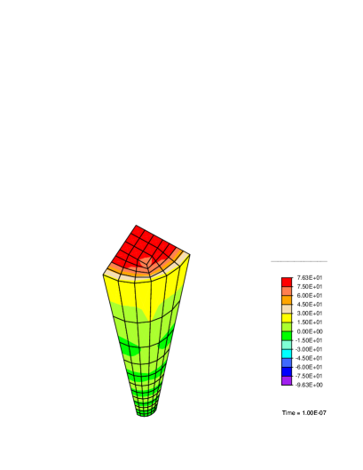
(b)

Figure 4: Longitudinal Cauchy stress, $\sigma_{33}$ (Pa) at $1\,\mathrm{nanosec.}$ and $100\,\mathrm{nanosec.}$ after the beginning of loading.

(a)

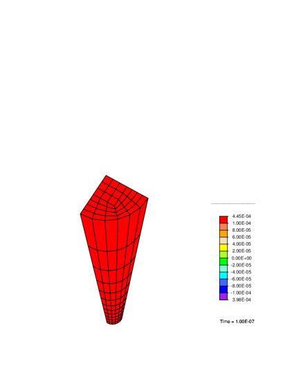
(b)

Figure 5: Stress gradient-driven flux ($\mathrm{kg.m}^{-2}\mathrm{sec}$) in the $\mbox{\boldmath$e$}_{3}$ direction at $1\,\mathrm{nanosec.}$ and $100\,\mathrm{nanosec.}$ after the beginning of loading. The positive values indicate an upward flux corresponding to a tensile $\sigma_{33}$ wave travelling downwards.

(a)

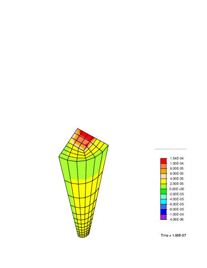
(b)

Figure 6: Internal energy gradient-driven flux, ($\mathrm{kg.m}^{-2}\mathrm{sec}$) in the $\mbox{\boldmath$e$}_{3}$ direction at $1\,\mathrm{nanosec.}$ and $100\,\mathrm{nanosec.}$ after the beginning of loading. The positive values indicate an upward flux. This corresponds to a lower energy near the top of the cylinder as the tensile stress ($\sigma_{33}$) wave travels downward and relaxes some of the strain energy of contraction.

(a)

(b)

Figure 7: Gravity-driven flux ($\mathrm{kg.m}^{-2}\mathrm{sec}$) in the $\mbox{\boldmath$e$}_{3}$ direction at $1\,\mathrm{nanosec.}$ and $100\,\mathrm{nanosec.}$ after the beginning of loading. The negative values indicate a downward flux, due to the action of gravity.

(a)

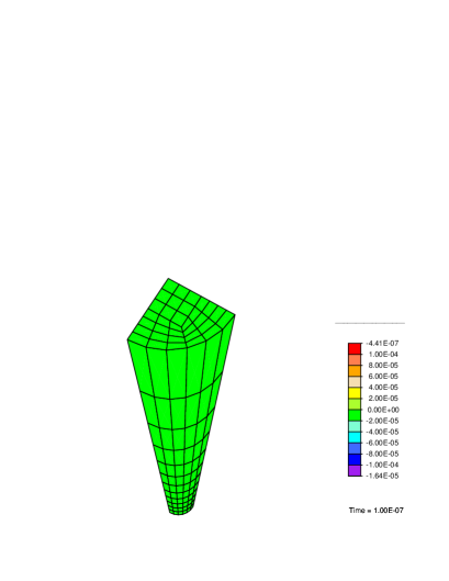
(b)

Figure 8: Inertia-driven flux ($\mathrm{kg.m}^{-2}\mathrm{sec}$) in the $\mbox{\boldmath$e$}_{3}$ direction at $1\,\mathrm{nanosec.}$ and $100\,\mathrm{nanosec.}$ after the beginning of loading. The negative values indicate a downward flux as the tissue accelerates upward.

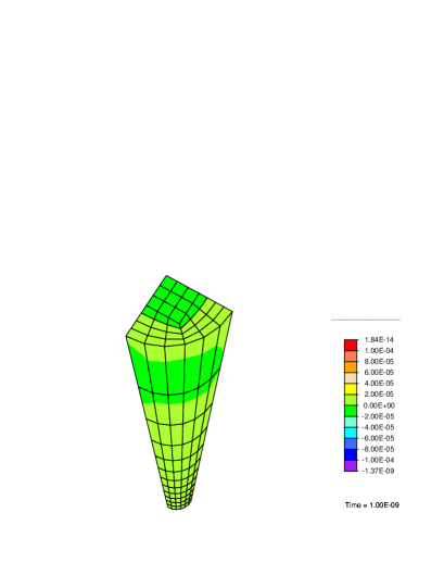
(a)

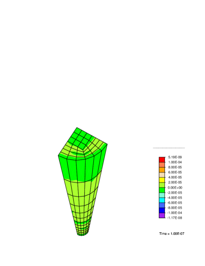
(b)

Figure 9: Concentration gradient-driven flux ($\mathrm{kg.m}^{-2}\mathrm{sec}$) in the $\mbox{\boldmath$e$}_{3}$ direction at $1\,\mathrm{nanosec.}$ and $100\,\mathrm{nanosec.}$ after the beginning of loading. Note that the maximum and minimum values are many orders of magnitude lower than for the other flux contributions reported above. This is a demonstration of mechanics influences dominating diffusion over the classical concentration gradient contribution.

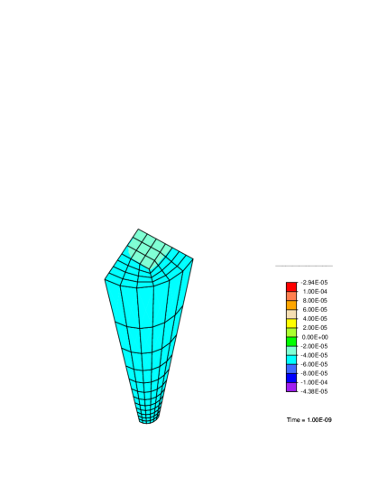
(a)

(b)

Figure 10: Total flux ($\mathrm{kg.m}^{-2}\mathrm{sec}$) in the $\mbox{\boldmath$e$}_{3}$ direction at $1\,\mathrm{nanosec.}$ and $100\,\mathrm{nanosec.}$ after the beginning of loading. The positive values indicate an upward flux, dominated by the stress gradient driven contribution.

The flux contributions in Figures 5–10 can be summarized as follows: The fluid flux is dominated by the contribution from the stress gradient in the $\mbox{\boldmath$e$}_{3}$ direction. The latter arises as the stress ($\sigma_{33}$) wave of tension travels down the cylinder in the first few microseconds after application of the load (the time taken to travel the length of the cylinder is $12\,\mu\mathrm{sec}$). Additionally, as the fluid concentration changes due to the flux, it causes a further change in the stress (Section 6). Other flux terms are qualitatively sensible; i.e., their directions are consistent with the physics of the problem, as argued in each of the figure captions. There is some loss of axial symmetry in a few of the plots due to the coarseness of the finite element mesh for this example. It appears that spatial oscillations in the solution lead to a further loss of symmetry in Figures 6b–7b and 10a. These oscillations arise due to large and dominant advective terms, and need to be remedied by stabilized finite element methods. Here, we only aim to demonstrate that various driving forces for mass transport are in agreement with their theoretical underpinnings in the paper. The resorption of the solid phase is shown indirectly in Figure 11. A positive fluid source, $\Pi^{\mathrm{f}}$, means that $\Pi^{\mathrm{s}}<0$. Since $\Pi^{\mathrm{s}}$ is the only term balancing $\partial\rho_{0}^{\mathrm{s}}/\partial t$ [see (2)], it follows that $\partial\rho_{0}^{\mathrm{s}}/\partial t<0$.

(a)

(b)

Figure 11: Rate of fluid production, $\Pi^{\mathrm{f}}$ ($\mathrm{kg.m}^{-3}.\mathrm{sec}^{-1}$), at $1\,\mathrm{nanosec.}$ and $100\,\mathrm{nanosec.}$ after the beginning of loading. The positive values indicate that the local fluid concentrations have fallen below their initial values.

8 Discussion and conclusions

A general framework for growth of biological tissue has been presented in this paper. While simplified models were used for source terms, $(\Pi^{\iota})$, they can be formulated on the basis of the kinetics of chemical reactions in order to develop more realistic growth laws. This approach, we believe, is fundamental to a proper treatment of mass transport in tissue. Results are obtained that differ fundamentally from the classical setting of continuum mechanics. Most notable among these differences are the mass fluxes driven by gradients in stress, strain, energy and entropy, in addition to body force and inertia. Importantly, though our treatment differs from classical mixture theory, the two are fully consistent as established at several points in this paper. The balance laws in Section 2 and 3 introduce a degree of coupling between the phenomena of mass transport and mechanics. This is visible most transparently in the balance of linear momentum (25) that includes mass fluxes, $\mbox{\boldmath$M$}^{\iota}$. The balance of mass, described by Equations (2) and (6), is also dependent upon the mechanics as the discussion in Section 6.1 makes clear. Notably, this ensures mechanics-mediated mass transport even with a mass source that is independent of strain/stress, as the discussion at the end of Section 6.3 establishes. The discussion in Sections 6.1–6.3 provides many insights into the nature of this coupling. The mechanics problem also has a constitutive dependence upon mass concentration, via (45) and the fact that the growth deformation gradient tensor, $\mbox{\boldmath$F$}^{\mathrm{g}^{\iota}}$ is determined by the concentration. The viscoelastic nature of the composite tissue would emerge naturally from a model incorporating a hyperelastic solid and viscous fluid.

We have formally allowed all species to be load bearing and develop a stress. At the scales that are of interest in a tissue, the only relevant load bearing species are the solid and fluid phases. Nevertheless, inasmuch as a transported species such as a nutrient has a molecular structure that can be subject to loads at the scale of pico-newtons, it is not inconsistent to speak of the partial stress of this species. Since the constitutive relation (45) indicates that the partial stresses are scaled by concentrations, the contribution to total stress from any species besides the solid and fluid phases will be negligible.

We have chosen to leave remodelling out of our formulation in this communication, to focus upon the above issues. Remodelling includes any evolution in properties, state of stress, material symmetry, volume or shape brought about by microstructural changes. In the development of biological tissue, growth and remodelling occur simultaneously. As density changes due to growth, the material also remodels by microstructural evolution within the neighborhood of each point. A rigorous treatment of this phenomenon has been presented in the continuum mechanical setting in a companion paper (Garikipati et al., 2003).

References

- Ambrosi and Mollica (2002) Ambrosi, D., Mollica, F., 2002. On the mechanics of a growing tumor. Int. J. Engr. Sci. 40, 1297–1316.
- Armero (1999) Armero, F., 1999. Formulation and fnite element implementation of a multiplicative model of coupled poro-plasticity at fnite strains under fully-saturated conditions. Comp. Methods in Applied Mech. Engrg. 171, 205–241.
- Baar et al. (2003) Baar, K., Birla, R., Boluyt, M. D., Borschel, G. H., Arruda, E. M., Dennis, R. G., 2003. Heart muscle by design: self-Organization of rat cardiac cells into contractile 3D cardiac tissue, submitted to Fed. Amer. Soc. Exp. Biol.
- Bedford and Drumheller (1983) Bedford, A., Drumheller, D. S., 1983. Recent advances: Theories of immiscible and structured mixtures. Int. J. Engr. Sci. 21, 863–960.
- Bilby et al. (1957) Bilby, B. A., Gardner, L. R. T., Stroh, A. N., 1957. Continuous distribution of dislocations and the theory of plasticity. In: Proceedings of the Ninth International Congress of Applied Mechanics, Brussels, 1956. Université de Bruxelles, pp. 35–44.
- Bischoff et al. (2002) Bischoff, J. E., Arruda, E. M., Grosh, K., 2002. A microstructurally based orthotropic hyperelastic constitutive law. J. Applied Mechanics 69, 570–579.
- Bustamante et al. (2003) Bustamante, C., Bryant, Z., Smith, S. B., 2003. Ten years of tension: Single-molecule DNA mechanics. Nature 421, 423–427.
- Calve et al. (2004) Calve, S., Baar, K., Grosh, K., Dennis, R. G., Arruda, E. M., 2004. Biochemical and mechanical characterization of engineered tendon, to appear in Proceedings of the XIV European Society of Biomechanics Conference, July 4–7, Hertogenbosch, The Netherlands.
- Calve et al. (2003) Calve, S., Dennis, R. G., Kosnik, P. E., Baar, K., Grosh, K., Arruda, E. M., 2003. Engineering of functional tendon, to appear in Tissue Engineering.
- Cowin and Hegedus (1976) Cowin, S. C., Hegedus, D. H., 1976. Bone remodeling I: Theory of adaptive elasticity. J. Elasticity 6, 313–326.
- de Boer (2000) de Boer, R., 2000. Theory of Porous Media: Highlights in the Historical Development and Current State. Springer, Berlin.
- de Groot and Mazur (1984) de Groot, S. R., Mazur, P., 1984. Nonequilibrium Thermodynamics. Dover.
- Epstein and Maugin (2000) Epstein, M., Maugin, G. A., 2000. Thermomechanics of volumetric growth in uniform bodies. International Journal of Plasticity 16, 951–978.
- Garikipati et al. (2001) Garikipati, K., Bassman, L. C., Deal, M. D., 2001. A lattice-based micromechanical continuum formulation for stress-driven mass transport in polycrystalline solids. Journal of Mechanics and Physics of Solids 49, 1209–1237.
- Garikipati et al. (2003) Garikipati, K., Narayanan, H., Arruda, E. M., Grosh, K., Calve, S., 2003. Material forces in the context of biotissue remodelling, to appear in Mechanics of Material Forces edited by P. Steinmann and G. A. Maugin, Kluwer Academic Publishers. e-print available at http://arXiv.org/abs/q-bio.QM/0312002.
- Gonzalez (1996) Gonzalez, O. C., July 1996. Design and analysis of conserving integrators for nonlinear Hamiltonian systems with symmetry. Ph.D. thesis, Stanford University.
- Guyton and Hall (1996) Guyton, A., Hall, J., 1996. Textbook of Medical Physiology. W.B. Saunders Company, Philadelphia.
- Harrigan and Hamilton (1993) Harrigan, T. P., Hamilton, J. J., 1993. Finite element simulation of adaptive bone remodelling: A stability criterion and a time stepping method. Int. J. Numer. Methods Engrg. 36, 837–854.
- Kuhl and Steinmann (2002) Kuhl, E., Steinmann, P., 2002. Geometrically nonlinear functional adaption of biological microstructures. In: Mang, H., Rammerstorfer, F., Eberhardsteiner, J. (Eds.), Proceedings of the Fifth World Congress on Computational Mechanics. International Association for Computational Mechanics, pp. 1–21.
- Lee (1969) Lee, E. H., 1969. Elastic-Plastic Deformation at Finite Strain. J. Applied Mechanics 36, 1–6.
- Lubarda and Hoger (2002) Lubarda, V. A., Hoger, A., 2002. On the mechanics of solids with a growing mass. Int. J. Solids and Structures 29, 4627–4664.
- Rajagopal and Wineman (1990) Rajagopal, K. R., Wineman, A. S., 1990. Developments in the mechanics of interactions between a fluid and a highly elastic solid. In: Kee, D. D., Kaloni, P. N. (Eds.), Recent Developments in Structured Continua. Vol. II. Longman Scientific and Technical, pp. 249–292.
- Rief et al. (1997) Rief, M., Oesterhelt, F., Heymann, B., Gaub, H. E., 1997. Single Molecule Force Spectroscopy on Polysaccharides by Atomic Force Microscopy. Science 275, 1295–1297.
- Simo and Tarnow (1992a) Simo, J. C., Tarnow, N., 1992a. Exact energy-momentum conserving algorithms and symplectic schemes for nonlinear dynamics. Comp. Methods in Applied Mech. Engrg. 100, 63–116.
- Simo and Tarnow (1992b) Simo, J. C., Tarnow, N., 1992b. The discrete energy-momentum method. conserving algorithm for nonlinear elastodynamics. Zeitschrift für Mathematik und Physik 43, 757–793.
- Simo et al. (1985) Simo, J. C., Taylor, R. L., Pister, K. S., 1985. Variational and projection methods for the volume constraint in finite deformation elasto-plasticity. Comp. Methods in Applied Mech. Engrg. 51, 177–208.
- Skalak (1981) Skalak, R. W., 1981. Growth as a finite displacement field. In: Carlson, D. E., Shields, R. T. (Eds.), Proceedings of the IUTAM Symposium on Finite Elasticity. Martinus Nijhoff, The Hague, Boston, London, pp. 347–355.
- Skalak et al. (1996) Skalak, R. W., Zargaryan, S., Jain, R. K., Netti, P. A., Hoger, A., 1996. Compatibility and the genesis of residual stress by volumetric growth. J. Math. Bio. 34, 889–914.
- Swartz et al. (1999) Swartz, M., Kaipainen, A., Netti, P. E., Brekken, C., Boucher, Y., Grodzinsky, A. J., Jain, R. K., 1999. Mechanics of interstitial-lymphatic fluid transport: Theoretical foundation and experimental validation. J. Bio. Mech. 32, 1297–1307.
- Taber (1995) Taber, L. A., 1995. Biomechanics of growth, remodelling and morphogenesis. Applied Mechanics Reviews 48, 487–545.
- Taber and Humphrey (2001) Taber, L. A., Humphrey, J. D., 2001. Stress-modulated growth, residual stress and vascular heterogeneity. J. Bio. Mech. Engrg. 123, 528–535.
- Taylor (1999) Taylor, R. L., September 1999. FEAP - A Finite Element Analysis Program. University of California at Berkeley, Berkeley, CA.
- Terzaghi (1943) Terzaghi, K., 1943. Theoretical Soil Mechanics. Wiley, New York; Chapman and Hall, London.
- Truesdell and Noll (1965) Truesdell, C., Noll, W., 1965. The Non-linear Field Theories (Handbuch der Physik, band III). Springer, Berlin.
- Truesdell and Toupin (1960) Truesdell, C., Toupin, R. A., 1960. The Classical Field Theories (Handbuch der Physik, band I). Springer, Berlin.
- Widmaier et al. (2003) Widmaier, E. P., Raff, H., Strang, K. T., 2003. Vander, Sherman and Luciano’s Human Physiology: The Mechanisms of Body Function, 9th Edition. McGraw Hill.