Abstract

Modern imaging techniques for probing brain function, including functional Magnetic Resonance Imaging, intrinsic and extrinsic contrast optical imaging, and magnetoencephalography, generate large data sets with complex content. In this paper we develop appropriate techniques of analysis and visualization of such imaging data, in order to separate the signal from the noise, as well as to characterize the signal. The techniques developed fall into the general category of multivariate time series analysis, and in particular we extensively use the multitaper framework of spectral analysis. We develop specific protocols for the analysis of fMRI, optical imaging and MEG data, and illustrate the techniques by applications to real data sets generated by these imaging modalities. In general, the analysis protocols involve two distinct stages: ‘noise’ characterization and suppression, and ‘signal’ characterization and visualization. An important general conclusion of our study is the utility of a frequency-based representation, with short, moving analysis windows to account for non-stationarity in the data. Of particular note are (a) the development of a decomposition technique (‘space-frequency singular value decomposition’) that is shown to be a useful means of characterizing the image data, and (b) the development of an algorithm, based on multitaper methods, for the removal of approximately periodic physiological artifacts arising from cardiac and respiratory sources.

Keywords: Spectral Analysis, functional magnetic resonance imaging (fMRI), optical imaging, magnetoencephalography (MEG), multivariate time series analysis, singular value decomposition.

1 Introduction

The brain constitutes a complex dynamical system with a large number of degrees of freedom, so that multichannel measurements are necessary to gain a detailed understanding of its behavior. Such multi-channel measurements, made available by current instrumentation, include multi-electrode recordings, optical brain images using intrinsic [Blasdel and Salama, 1986], [Grinvald et al., 1992] or extrinsic [Davila et al., 1973] contrast agents, functional magnetic resonance imaging (fMRI) [Ogawa et al., 1992],[Kwong et al., 1992] and magnetoencephalography (MEG) [Hamalainen et al., 1993]. Due to improvements in the capabilities of the measuring apparatus, as well as growth in computational power and storage capacity, the data sets generated by these experiments are increasingly large and more complex. The analysis and visualization of such multichannel data is an important piece of the associated research program, and is the subject of this paper.

There are several common problems associated with the different types of multichannel data enumerated above. Firstly, preprocessing is necessary to remove nuisance components, arising from both instrumental and physiological sources, from the data. Secondly, an appropriate representation of the data for purposes of analysis and visualization is necessary. Thirdly, there is the task of extracting any underlying simplicities from the signal, mostly in absence of strong models for the dynamics of the relevant parts of the brain. If there are simple features that are hidden in the complexity of the data, then the analytical methodology should be such as to reveal such features efficiently.

With the current exponential growth in computational power and storage capacity, it is increasingly possible to perform the above steps in a semi-automated way, and even in real time. In fact, this is almost a pre-requisite to the success of multi-channel measurements, since the large dimensionality of the data sets effectively preclude exhaustive manual inspection by the human experimenter. An additional challenge is to perform the above steps as far as possible in real time, thus allowing quick feedback into the experiment. The intimate interplay between the basic experimental apparatus and semi-automated analysis and visualization is schematically illustrated in Fig.1. Note that even given the increases in storage capacity, it is desirable to have ways of compressing the data while retaining the appropriate information, so as to prevent saturation of the available storage.

Problems such as the above are clearly not unique to neuroscience. Automated analysis plays an important role in the emergent discipline of computational molecular biology. Despite the current relevance of these problems, the appropriate analytical and computational tools are in an early stage of development. In addition, investigators in the field are sometimes unaware of the appropriate modern signal processing tools. Since little is understood about the detailed workings of the brain, a straightforward exploratory approach using crude analysis protocols is usually favored. However, given the increasing availability of computational resources, this unnecessarily limits the degree of knowledge that can be gained from the data, and at worst can lead to erroneous conclusions, for example when statistical methods are applied inappropriately (cf.[Cleveland, 1993] p.177). On the other hand, a superficial application of complex signal processing or statistical techniques, can lead to results that are difficult to interpret.

An aspect of the the data in question that cannot be emphasized enough is the fact that the data constitute time series, mostly multivariate. While techniques for treating static high-dimensional data are widely known and appreciated, both in multivariate statistics and in the field of pattern recognition, the techniques for treating time series data are less well developed, except in special cases. We focus particularly on the data as multivariate time series. In this paper, our concerns are twofold: (a) characterization and removal of the typical artifacts, and (b) characterization of underlying structure of the signal left after removal of artifacts. The paper is organized into two parts.

Figure 1: Schematic overview of data acquisition and analysis

In the first part we review some of the relevant analytical techniques for multivariate time series. In particular, we provide a description of multitaper spectral methods [Thomson, 1982], [Thomson and Chave, 1991], [Percival and Walden, 1993]. This is a framework for performing spectral analysis of univariate and multivariate time series that has particular advantages for the data at hand. A central issue for the data we present is to be able to deal with very short data segments and still obtain statistically well behaved estimators. Reasons for this are that gathering long time series may be expensive (for example in fMRI), and that the presence of non-stationarity in the data makes it preferable to use a short, moving analysis window. Multitaper methods are particularly powerful for performing spectral analysis of short data segments. In the second part of the paper, we treat in succession dynamic brain imaging data gathered in MEG, optical and fMRI experiments. Based on the analysis of actual data sets using the techniques introduced in the first section, we discuss protocols for analysis, both to remove artifactual components as well as to determine the structure of the signal.

A principal motivation for the current study is the increasing interest in the internal dynamics of neural systems. In many experimental paradigms, past or present, neural systems have been characterized from the point of view of input-output relationships. For example, the quantity of interest is often a stimulus response, and the experiment is performed by repeating the stimulus multiple times, and the different trials are regarded as forming a statistical ensemble. However, the trial to trial fluctuations, and more generally the spontaneous fluctuations of the neural system in question, are not necessarily completely random, and quite often have explicit structure, such as oscillations. Understanding these ”baseline fluctuations” may be quite important in learning about the dynamics of neural systems, even in the context of response to external stimuli. To characterize these spontaneous fluctuations is a more difficult task than learning input-output relationships. The analytical techniques developed in this paper should be of utility in such characterization for multichannel neural data, particularly dynamic brain images.

2 Different Brain Imaging Techniques

2.1 Imaging techniques and their spatiotemporal resolution

The three main techniques of interest here are optical imaging, fMRI and MEG. Optical imaging falls into the further sub-categories of intrinsic and extrinsic contrast. In extrinsic contrast optical imaging, an optical contrast agent sensitive to neuronal activity is added to the preparation. Examples of such contrast agents include voltage-sensitive dyes and $Ca^{2+}$ concentration sensitive contrast agents. Voltage-sensitive dye molecules insert in the cell membrane and the small Stark shifts produced in the molecule by changes in the transmembrane voltage are sources of the contrast. The signal to noise ratio (SNR) in these experiments is typically poor, being of the order of unity. The spatial resolution is set by the optical resolution and scattering properties of the medium and can be of the order of microns. The temporal resolution is limited by the digitization rate of the recording apparatus (CCD camera or photodiode array) and can currently go up to $\sim 1kHz$, which is the intrinsic timescale of neuronal activity. In calcium ion sensitive imaging, the intrinsic timescales are slower, so that the demands on the digitization rate are somewhat less. The signal to noise ratio is significantly better compared to currently available voltage-sensitive dyes. The spatial resolution is greatly enhanced in confocal [Pawley, 1995] and multi-photon scanning optical imaging [Denk et al., 1990]. The imaging rates in multi-photon scanning optical imaging are currently significantly slower than the corresponding rates for CCD cameras.

Intrinsic optical imaging and fMRI rely on the same underlying mechanism, namely hemodynamic changes triggered by neuronal activity. Hemodynamic changes include changes in blood flow and blood oxygenation level. The intrinsic timescale for these changes is slow, ranging from hundreds of milliseconds to several seconds. The intrinsic spatial scale is also somewhat large, ranging from hundreds of microns to millimeters. These scales are well within the scope of optical techniques. In both the extrinsic and intrinsic cases discussed above, various noise sources including physiological fluctuations are important indirect determinants of the spatiotemporal resolution.

In fMRI, the instrumental limitations on the spatial and temporal resolutions are significant, and for fixed SNR, a tradeoff exists between spatial and temporal resolution, as well as between temporal resolution and spatial coverage. The fMRI images are typically gathered in two dimensional slices of finite thickness, and for a fixed SNR, the number of slices is roughly linear in time. For single slice experiments, the temporal resolution is $\sim 100ms$, and the spatial resolution is $\sim 1mm$. This spatial resolution can be improved for a single slice by sacrificing temporal resolution. For multiple slices covering the whole head, the temporal resolution is $\sim 2s$. Note that these numbers may be expected to change somewhat based on future improvements in instrumentation. The principal advantage of fMRI is that it is non-invasive imaging, making it suitable for the study of the human brain. In addition, optical imaging is limited to the surface of the sample, whereas fMRI is a volumetric imaging technique.

In MEG, weak magnetic fields of the order of tens of $fT/\sqrt{(}Hz)$ generated by electric currents in the brain are measured using superconducting quantum interfometric detector (SQUID) arrays positioned on the skull. Like fMRI, MEG is a noninvasive imaging technique and therefore applicable to the human brain. The temporal resolution ($\sim 1ms$) is much higher than in fMRI, although the spatial resolution is in general significantly poorer. The spatial resolution of MEG remains a debatable issue, due to the ill-posed nature of the inverse problem that must be solved in order to obtain an image from the MEG data. A promising direction for future research appears to be a combined use of fMRI and MEG, performed separately on the same subject.

2.2 Sources of noise

As mentioned previously, the ‘noise’ present in the imaging data arise from two broad categories of sources, biological and non-biological. Biological noise sources include cardiac and respiratory cycles, as well as motion of the experimental subject. In imaging studies involving hemodynamics such as fMRI and intrinsic optical imaging, an additional physiological source of noise are slow ‘vasomotor’ oscillations [Mitra et al., 1997], [Mayhew et al., 1996]. In addition in all studies of evoked activity, ongoing brain activity not locked to or triggered by the stimulus appears as ‘noise’. Non-biological noise sources include photon counting noise in optical imaging experiments, noise in the electronic instrumentation, 60 cycle noise, building vibrations and the like.

We first consider optical imaging using voltage-sensitive dyes in animal preparations. These sensitivity of these experiments is currently limited by photon counting noise. The Stark shifts associated with the available dyes lead to changes in the optical fluorescence signal on the order of $\Delta F/F\sim 10^{-3}/mV$. The typical signal-to-noise ratio is therefore of order unity or less. In addition, absorption changes arising from hemodynamic sources, whether related to the stimulus or not, corrupt the voltage-sensitive dye images. Perfusing the brain with an artificial oxygen-supplying fluid can eliminate these artifacts [Prechtl et al., 1997]. Motion artifacts and electronic noise may also be significant. In contrast, Ca-sensitive dye images have comparitively large signal changes for spike mediated $Ca^{2+}$ fluxes and are less severely affected by the photon counting noise. However motion artifacts can still be severe, particularly at higher spatial resolutions.

In fMRI experiments in humans, the instrumental noise is small, typically a fraction of a percent. The dominant noise sources are of physiological origin, mainly cardiac, respiratory and vasomotor sources [Mitra et al., 1997]. Depending on the time between successive images, these oscillations may be well resolved in the frequency spectrum, or aliased and smeared over the sampling frequency interval. Subject motion, due to respiration or other causes, is a major confounding factor in these experiments.

In MEG experiments the signal-to-noise ratio is usually very low. Hundreds of trial averages are sometimes needed to extract evoked responses. Magnetic fields due to currents associated with the cardiac cycle are a strong noise source, as are 60 cycle electrical sources and other non-biological current sources. In studying the evoked response, the spontaneous activity not related to the stimulus is a dominant source of undesirable fluctuations.

3 Description of data sets

In this section we describe the data sets used to illustrate the techniques developed in the paper. We have used data from three different imaging techniques, corresponding to multichannel MEG recordings, optical image time series, and MRI time series. The data are grouped into four sets, referred to below using the letters $\mathcal{A}$ through $\mathcal{D}$. Brief discussions of the data collection are provided below. The data have either been previously reported or are gathered using the same techniques as in other reports. In each case, a more detailed description may be found in the accompanying reference.

Data set $\mathcal{A}$ consists of multichannel MEG recordings. Descriptions of the apparatus and experimental methods for these data can be found in [Joliot et al., 1994]. For our purposes it is sufficient to note that the data were gathered simultaneously from 74 channels using a digitization rate of $2.083kHz$ for a total duration of $5$ minutes, and corresponds to magnetic fields due to spontaneous brain activity recorded from an awake human subject in a resting state with eyes closed.

Data set $\mathcal{B}$ consists of dynamic optical images of the procerebral lobe of the terrestrial mollusc Limax [Kleinfeld et al., 1994], gathered after staining the lobe with a voltage-sensitive dye. The digitization rate is $75Hz$ and the total duration of the recording is $23s$. The images are $105\times 34$ pixels in extent and cover an area of approximately $600\mu m\times 200\mu m$.

Data sets $\mathcal{C}$ and $\mathcal{D}$ contain fMRI data, and consist of time series of magnetic resonance images of the human brain showing a coronal slice towards the occipital pole [Mitra et al., 1997], [Le and Hu, 1996]. The data were gathered in the presence ( $\mathcal{C}$ ) or absence ( $\mathcal{D}$ ) of a visual stimulus. For data set $\mathcal{C}$, binocular visual stimulus was provided by a pair of flickering red LED patterns ($8Hz$), presented for $30$ seconds starting $40$ seconds after the beginning of image acquisition. The digitization rate for the images was $5Hz$ and the total duration $110s$. The images are $64\times 64$ pixels and cover a field of view of $20cm\times 20cm$.

4 Analysis Techniques

4.1 Time Series Analysis Techniques

Here we briefly review some methods used to analyze time series data. The aim here is not to provide a complete list of the relevant techniques, but discuss those methods which are directly relevant to the present work. In particular, in the next section, we provide a review of multitaper spectral analysis techniques [Thomson, 1982], [Percival and Walden, 1993], since these are used in the present paper, and are not widely known.

The basic example to be considered is the power spectral analysis of a single (scalar) time series, or an output scalar time series given an input scalar time series. The relevant analysis techniques can be generally categorized under two different attributes: linear or non-linear, and parametric or non-parametric. We will mostly be concerned with multitaper spectral techniques, for which the attributes are linear and non-parametric. Although we categorize the techniques as linear, note that spectra are quadratic functions of the data. Also, some of the spectral quantities we consider are other nonlinear functions of the data. We prefer non-parametric spectral techniques (eg. multitaper spectral estimates) over parametric ones (eg. autoregressive spectral estimates, also known as maximum entropy spectral estimates, or linear predictive spectral estimates). Some weaknesses of parametric methods in the present context are lack of robustness and lack of sufficient flexibility to fit data with complex spectral content. The reader is referred to the literature for a comparison between parametric and non-parametric spectral methods [Thomson, 1982], [Percival and Walden, 1993], and we also discuss this issue further below.

We also do not use methods, based on time lag or delay embeddings, that characterize neurobiological time series as outputs of underlying nonlinear dynamical systems. These methods work if the underlying dynamical system is low dimensional, and if one can obtain large volumes of data so as to enable construction of the attractor in phase space. The amount of data needed grows exponentially with the dimension of the underlying attractor. On the one hand, it is true that neurobiological time series are outputs of rather nonlinear dynamical systems. However, in most cases it is not clear that the constraint of low dimensionality is met, except perhaps for very small networks of neurons. In cases where the dynamics may appear low dimensional for a short time, non-stationarity is a serious issue, and precludes acquisition of very long stretches of data. One might think that non-stationarity could be accounted for by simply including more dynamical degrees of freedom. However, that also would require the acquisition of exponentially larger data sets. We constrain ourselves to spectral analysis techniques as opposed to the techniques indicated above. The reason for this is twofold: Firstly, spectral analysis remains a fundamental component of the repertoire of tools applied to these problems, and as far as we are concerned, the appropriate spectral techniques have not been sufficiently well studied or utilized in the present context. Secondly, it remains debatable whether much progress has been made in understanding the systems involved using the nonlinear techniques [Theiler and Rapp, 1996], [Rapp et al., 1994].

4.1.1 Time domain versus Frequency domain: Resolution and Non-stationarity

In the neurobiological context, data are often characterized in terms of appropriate correlation functions. This is equivalent to computing corresponding spectral quantities. If the underlying processes are stationary, then the correlation functions are diagonal in frequency space. For stationary processes, local error bars can be imposed for spectra in the frequency domain, whereas the corresponding error bars for correlation functions in the time domain are non-local [Percival and Walden, 1993]. In addition, if the data contains oscillatory components, which is true for the data treated here, they are compactly represented in frequency space. These reasons form the basis for using a frequency-based representation. For some other advantages of spectra over autocovariance functions, see [Percival and Walden, 1993] pp. 147-149. The arguments made here are directly applicable to the continuous processes that are of interest in the current paper. Similar arguments also apply to the computation of correlation functions for spike trains. An exception should be made for those spike train examples where there are sharp features in the time domain correlation functions, e.g. due to monosynaptic connections. However, broader features in spike train correlation functions would be better studied in the frequency domain, a point that is not well appreciated.

Despite the advantages of the frequency domain indicated above, the frequent presence of non-stationarity in the data, makes it necessary in most cases to use a time-frequency representation. In general, the window for spectral analysis is chosen to be as short as possible to be consistent with the spectral structure of the data, and this window is translated in time. Fundamental to time-frequency representations is the uncertainty principle, which sets the bounds for simultaneous resolution in time and frequency. If the time-frequency plane is ‘tiled’ so as to provide time and frequency resolutions $\Delta t$ by $\Delta f$, then $\Delta t\Delta f\geq 1$. Although there has been a lot of work involving tilings of the time-frequency plane using time-scale representations (wavelet bases), we choose to work with frequency rather than scale as the basic quantity, since the time series we are dealing with are better described as having structure in the frequency domain. In particular, the spectra typically have large dynamic range (which indicates good compression of data in the frequency space), and also have spectral peaks, rather than being scale invariant. The time-frequency analysis is often crucial to see this structure, since a long time average spectrum may prove to be quite featureless. An example of this is presented by MEG data discussed below.

4.1.2 Digitization rate, Nyquist Frequency, Fourier Transforms

Some quantites that are central to the discussion are defined below. Consider a time series window of length $T$. The frequency resolution is given by the so-called Raleigh frequency, $\delta f=1/T$. In all real examples, the time series is obtained at discrete time locations. If we assume the discrete time locations are uniformly spaced at intervals of $\Delta t$, then the number of time points $N$ in the interval $T$ is given by $N=T/(\Delta t)$. The digitization frequency or digitization rate is by definition $1/(\Delta t)$. An important quantity is the Nyquist frequency $f_{Nyq}$, defined as half the digitization frequency $f_{Nyq}=1/(2\Delta t)$. In this context, it is important to recall the Nyquist theorem and the related concept of aliasing. The basic idea of the Nyquist theorem is that the digitized time series is a faithful representation of the original continuous time series as long as the the original time series does not contain any frequency components above the Nyquist frequency. Put in a different way, a continuous time series which is band limited to the interval $[-B,B]$, should be digitized at a rate $2B$ (i.e. $\Delta t=1/(2B)$) in order to retain all the information present in the continuous time series. Aliasing is an undesirable effect that occurs if this criterion is violated, namely if a time series with frequency content outside the frequency interval $[-f_{Nyq},f_{Nyq}]$ is digitized at an interval $\Delta t=2/f_{Nyq}$. The spectral power outside the specified interval is then ‘aliased’ back into the interval $[-f_{Nyq},f_{Nyq}]$. Consequently the Nyquist theorem tells us how frequently a continuous time series should be digitized. These concepts are fundamental to the discussion, and the reader unfamiliar with them would benifit from consulting an appropriate text (e.g. see [Percival and Walden, 1993]).

The Fourier transform $\tilde{x}(f)$ of a discrete time series $\{x_{t}|t=n\Delta t,n=1,2,...,N\}$ is defined in this paper as

$$\tilde{x}(f)=\sum_{n=1}^{N}x_{t}e^{-2\pi ifn\Delta t}$$ (1)

In places where we use the convention $\Delta t=1$ the above equation may be rewritten replacing $n$ by $t$ as

$$\tilde{x}(f)=\sum_{t=1}^{N}x_{t}e^{-2\pi ift}$$ (2)

The corresponding Nyquist frequency is dimensionless and numerically equal to $1/2$. In any real application, of course, both the digitization rate and the Nyquist frequency have appropriate units. The total time window length $T$ now becomes interchangeable with $N$. More generally, $T=N\Delta t$ as above. One frequent source of confusion is between the Fourier transform defined above and the Fast Fourier Transform (FFT). The FFT is an algorithm to efficiently compute the Fourier transform on a discrete grid of time points, and should not be confused with the Fourier transform which is the underlying continuous function of frequency defined above.

4.1.3 Conventional Spectral Analysis

In this and subsequent subsections, we set $\Delta t=1$, $T=N$. Physical units are restored where appropriate. We consider below a model example of a time series constructed by adding a stochastic piece, consisting of an autoregressive process excited by white Gaussian noise, to three sinusoids. The time series is given by $y_{t}=x_{t}+\sum_{k=1}^{3}A_{k}\sin(2\pi f_{k}t+\phi_{k})$, where $t=1,2,..,N$ with N=1024, and the parameters of the sinusoids are $A_{k}=(0.7,0.7,0.08)$, $f_{k}=(0.122,0.391,0.342)$ and $\phi_{k}=(0,\pi/3,2\pi/3)$ for $k=(1,2,3)$. Here $x_{t}$ is an autoregressive process of order 4 given by $x_{t}=\sum_{k=1}^{4}a_{k}x_{t-k}+\epsilon_{t}$, with $a_{k}=(-0.683,1.55,-1.96,1.87)$. For successive time samples $t$, $\epsilon_{t}$ are independently drawn from a normal distribution with unit variance. In Fig. 2, the first 300 points of the time series example are plotted.

Figure 2: Piece of a time series composed of a stochastic piece generated by an order 4 autoregressive process added to a sum of three sinusoids (see text).

Figure 3: Autoregressive spectral estimate of time series data shown in Figure 2 (dashed line). Also shown is the theoretical spectrum of the underlying process (solid line). Note that the sine waves lead to delta functions, whose heights have been determined for the display so that the integrated intensity over a Raleigh frequency gives the correct strength of the theoretical delta function. The autoregressive estimate completely misses the peaks at $f=0.122$ and $f=0.391$.

In conventional non-parametric spectral analysis a tapered Fourier transform of the data is used to estimate the power spectrum. There are various choices of tapers. A taper with optimal bandlimiting properties is the zero^th discrete prolate spheroidal sequence which is described in detail later in the text. Using this taper, a single taper spectral estimate is given in the top right corner of Fig. 5. In this and the following section, the Fourier transforms are implemented using an FFT after the time series of length $N$ is padded out to length $4N$ or $8N$. This still gives a discrete representation of the corresponding continuous functions of frequency, however the grid is sufficiently fine that the resulting function appears to be smooth as a function of frequency.

4.1.4 Autoregressive spectral estimation

To illustrate a parametric spectral estimate, we show in Fig. 3 the results of an autoregressive (AR) modelling of the data using an order 19 AR process. We used the Levinson-Durbin procedure for purposes of this illustration [Percival and Walden, 1993] p.397. The order of the AR model was determined using the criterion AIC [Akaike, 1974]. Although the parametric estimate is smooth, it fails to accurately estimate the underlying theoretical spectrum. In particular, it completely misses the delta function peaks at $f=0.122$ and $f=0.391$.

Some comments are in order regarding AR spectral estimates. The basic weakness of this method is that it starts with the correlation function of the data in order to compute the AR coefficients. This, however, presupposes the answer, since the correlation function is nothing but the Fourier transform of the spectrum - if the correlation function were actually known, there would be no need to estimate the spectrum. In practice, an estimate of the correlation function is made from the data, which contains the same bias problems as in estimating spectra. In fact, in obtaining the illustrated fit, we computed the correlation function by Fourier transforming a direct multitaper spectral estimate (to be described below). Attempts to escape from the circularity pointed out above usually result in strong model assumptions, which then lead to misfits in the spectra (for further discussions, see [Thomson, 1990], p.614). Despite these problems, AR methods do have some use in spectral estimation, namely to obtain pre-whitening filters that reduce the dynamic range of the process and thus helps reduce bias in the final spectral estimate. Another valid usage of AR methods is to treat sufficiently narrowband signals that can be appropriately modeled by low order AR processes.

4.1.5 Multitaper Spectral Analysis

Here we present a brief review of multitaper estimation [Thomson, 1982]. This method involves the use of multiple orthogonal data tapers, in particular prolate spheroidal functions, which provide a local eigenbasis in frequency space for finite length data sequences. A summary of the advantages of this technique can be found in Percival and Walden [Percival and Walden, 1993], Chapter 7.

Figure 4: Left column: prolate spheroidal data tapers for $NW=5$ (k=1…4). Right column: tapered time series corresponding to the time series in the example given in the text (part of which is shown in Fig.2), multiplied by the data tapers in the left column.

Figure 5: Left column: spectra of the data tapers shown in Fig.4, left column. Right column: spectra of the tapered time series shown in Fig.4, right column, giving single taper estimates of the spectrum.

Consider a finite length sample of a discrete time process $x_{t}$, $t=1,2,\ldots,N$. Let us assume a spectral representation for the process,

$$x_{t}=\int_{-\mbox{\small$\frac{1}{2}$}}^{\mbox{\small$\frac{1}{2}$}}dX(f)e^{2\pi ift}$$ (3)

The Fourier transform of the data sequence $\tilde{x}(f)$ is therefore given by

$$\tilde{x}(f)=\sum_{1}^{N}x_{t}e^{-2\pi ift}=\int_{-\mbox{\small$\frac{1}{2}$}}^{\mbox{\small$\frac{1}{2}$}}K(f-f^{\prime},N)dX(f^{\prime})$$ (4)

where

$$K(f-f^{\prime},N)=e^{-2\pi i(f-f^{\prime})(N+1)/2}{\sin(N\pi(f-f^{\prime}))\over\sin(\pi(f-f^{\prime}))}$$ (5)

Note that for a stationary process, the spectrum is given by $S(f)df=E[|dX(f)|^{2}]$. A simple estimate of the spectrum (apart from a normalization constant) is obtained by squaring the Fourier transform of the data sequence, i.e. $|\tilde{x}(f)|^{2}$. This suffers from two difficulties: Firstly, $\tilde{x}(f)$ is not equal to $X(f)$ except when the data length is infinite, in which case the kernel in Eq.5 becomes a delta function. Rather, it is related to $X(f)$ by a convolution, as given by Eq.4. This problem is usually referred to as ‘bias’, and corresponds to a mixing of information from different frequencies of the underlying process due to a finite data window length. Secondly, even if the data window length were infinite, calculating $|\tilde{x}(f)|^{2}$ without using a tapering function (a quantity known as the periodogram) effectively squares the observations without averaging - the spectrum is the expectation of this squared quantity. This issue is referred to as the lack of consistency of the periodogram estimate, namely the failure of the periodogram to converge to the spectrum for large data lengths. The reason for this is straightforward. When one takes a fast Fourier transform of the data, one is estimating $N$ quantities from $N$ data values, which obviously leads to overfitting if the data is stochastic. More precisely, the squared Fourier transform of the time series is an inconsistent estimator of the spectrum, because it does not converge as the data time series tends to infinite length.

To resolve the first issue, the data is usually multiplied by a data taper, which leads to replacing the kernel in Eq.5 by a kernel that is more localized in frequency. However, this leads to the loss of the ends of the data. To surmount the second problem, the usual approach is to average together overlapping segments of the time series [Welch, 1967]. Repetition of the experiment also gives rise to an ensemble over which the expectation can be taken, but we are interested in single trial calculations which involve only a single time series. Evidently, some amount of smoothing is necessary to reduce the variance of the estimate, the question being what is an appropriate and systematic way to performing this smoothing.

An elegant approach towards the solution to both of the above problems is provided by the multitaper spectral estimation method in which the data is multiplied by not one, but several orthogonal tapers, and Fourier transformed to obtain the basic quantity for further spectral analysis. The method can be motivated by treating Eq.4 as an integral equation to be solved in a regularized way. The simplest example of the method is given by the direct multitaper spectral estimate $S_{MT}(f)$, defined as the average over individual tapered spectral estimates,

$$S_{MT}(f)={1\over K}\sum_{k=1}^{K}|\tilde{x}_{k}(f)|^{2}$$ (6)

where

$$\tilde{x}_{k}(f)=\sum_{1}^{N}w_{t}(k)x_{t}e^{-2\pi ift}$$ (7)

Figure 6: Direct multitaper spectral estimate of time series example using $WT=5$, $K=9$. The estimates for the first four of the nine tapers that are averaged to create this estimate is shown in Fig.5. The theoretical spectrum is also shown.

Here $w_{t}(k)~{}(k=1,2,\ldots,K)$ are $K$ orthogonal taper functions with appropriate properties. A particular choice of these taper functions, with optimal spectral concentration properties, is given by the Discrete Prolate Spheroidal Sequences (DPSS) [Slepian and Pollak, 1961]. Let $w_{t}(k,W,N)$ be the $k^{th}$ Discrete Prolate Spheroidal Sequence (DPSS) of length $N$ and frequency bandwidth parameter $W$. The DPSS form an orthogonal basis set for sequences of length, $N$, and are characterized by a bandwidth parameter $W$. The important feature of these sequences is that for a given bandwidth parameter $W$ and taper length $N$, $K=2NW$ sequences out of a total of $N$ each have their energy effectively concentrated within a range $[-W,W]$ of frequency space. Consider a sequence $w_{t}$ of length $N$ whose Fourier transform is given by $U(f)=\sum_{1}^{N}w_{t}e^{-2\pi ift}$. Then we can consider the problem of finding sequences $w_{t}$ so that the spectral amplitude $U(f)$ is maximally concentrated in the interval $[-W,W]$, i.e.

$$\int_{-W}^{W}|U(f)|^{2}df$$ (8)

is maximized, subject to a normalization constraint which may be imposed using a Lagrange multiplier. It can be shown that the optimality condition leads to a matrix eigenvalue equation for $w_{t}(k,W,N)$

$$\sum_{t^{\prime}=1}^{N}{\sin\bigl{[}2\pi W(t-t^{\prime})\bigr{]}\over\pi(t-t^{\prime})}w_{t^{\prime}}=\lambda w_{t}$$ (9)

The eigenvectors of this equation are the DPSS. The remarkable fact is that the first $2NW$ eigenvalues $\lambda_{k}(N,W)$ (sorted in descending order) are each approximately equal to one, while the remainder are approximately zero. Since it follows from the above definitions that

$$\lambda_{k}(N,W)={\int_{-W}^{W}|U(f)|^{2}df\over\int_{-{1\over 2}}^{1\over 2}|U(f)|^{2}df}$$ (10)

this is a precise statement of the spectral concentration mentioned above. The fact that many of the eigenvalues are close to one makes the eigenvalue problem Eq.9 ill-conditioned and unsuitable for the actual computation of the prolates (this can be achieved by a better conditioned tridiagonal form [Percival and Walden, 1993]). The DPSS can be shifted in concentration from $[-W,W]$ centered around zero frequency to any non-zero center frequency interval $[f_{0}-W,f_{0}+W]$ by simply multiplying by the appropriate phase factor $e^{2\pi if_{0}t}$, an operation known as demodulation. The usual strategy is to select the desired analysis half-bandwidth $W$ to be a small multiple of the Raleigh frequency $1/N$, and then take the leading $2NW-1$ DPSS as data tapers in the multitaper analysis. Note that less than $2NW$ of the sequences are typically taken, since the last few of these have progressively worsening spectral concentration properties.

For illustration, in the left column of Fig. 4, we show the first $4$ DPSS for $W=5/N$. Note that the orthogonality condition ensures that successive DPSS each have one more zero crossing than the previous one. In the right column of Fig. 4, we show the time series example from the earlier subsection multiplied by each of the successive data tapers. In the left column of Fig. 5, we show the spectra of the data tapers themselves, showing the spectral concentration property. The vertical marker denotes the bandwidth parameter $W$

In Fig. 5, we show the magnitude squared Fourier transforms of the tapered time series shown in Fig. 4. The arithmetic average of these spectra for $k=1,2,\ldots,9$ (note that only 4 out of 9 are shown in Figs. 4 and 5) give a direct multitaper estimate of the underlying process, shown in Fig.6. Also shown in that figure is the theoretical spectrum of the underlying model.

In the direct estimate, an arithmetic average of the different spectra is taken. However, the different data tapers differ in their spectral sidelobes, so that a weighted average is more appropriate. In addition, the weighting factors should be chosen adaptively depending on the local variations in the spectrum. For more detailed considerations along these lines, the reader is referred to [Thomson, 1982].

$(a)$    $(b)$

Figure 7: a) F-statistic values for testing for the presence of a significant sinusoidal component in the time series example along with significance levels. b) Direct multitaper spectral estimate of the time series example using $WT=5$, $K=9$ reshaped to remove the sinusoidal lines. The theoretical spectrum is also shown in bold.

Sine waves in the original time series correspond to square peaks in the multitaper spectral estimate. This is usually an indication that the time series contains a sinusoidal component along with a broad background. The presence of such a sinusoidal component may be detected by a test based on a goodness-of-fit F-statistic [Thomson, 1982]. To proceed, let us assume that the data contains a sinusoid of complex amplitude $\mu$ at frequency $f_{0}$ (The corresponding real series being $Re(\mu e^{2\pi if_{0}t})$). Let us also assume that in a frequency interval $[f_{0}-W,f_{0}+W]$ around $f_{0}$, the process, to which the sinusoid is added, is white. Note that this is a much weaker assumption than demanding that the process is white over the entire frequency range. Under these assumptions, for $f\epsilon[f_{0}-W,f_{0}+W]$ the tapered Fourier transforms of the data are given by

$$\tilde{x}_{k}(f)=\mu U_{k}(f-f_{0})+n_{k}(f),~{}~{}~{}k=1,2,\ldots,K$$ (11)

Here $U_{k}(f)$ is the Fourier transform of the $k^{th}$ DPSS, and f is in the range $[f_{0}-W,f_{0}+W]$. The assumption of a locally white background implies that $n_{k}(f)$ are independently and indentically distributed complex Gaussian variables. Treating Eq.11 as a linear regression equation at $f=f_{0}$ leads to an estimate of the sine wave amplitude (which corresponds to a particular tapered Fourier transform of the data)

$$\hat{\mu}(f_{0})={\sum_{k}x_{k}(f_{0})U_{k}^{*}(0)\over\sum_{k}|U_{k}(0)|^{2}}$$ (12)

and to an $F$ statistic for the significance of a non-zero $\mu$

$$F(f_{0})={|\hat{\mu}(f_{0})|^{2}\over\sum_{k}|\tilde{x}_{k}(f_{0})-\hat{\mu}(f_{0})U_{k}(0)|}$$ (13)

Under the null hypothesis that there is no line present, $F(f_{0})$ has an $F$ distribution with $(2,2K-2)$ degrees of freedom. We plot this function $F(f)$ for the time series in the above example in Fig. 7(a). For this example, we have chosen $W=7/N$, $K=13$. One obtains an independent $F$ statistic every Raleigh frequency, and since there are $N$ Raleigh frequencies in the spectrum, the statistical significance level is chosen to be $1-1/N$. This means that on an average, there will be at most one false detection of a sinusoid across all frequencies. A horizontal line in Fig. 7(a) indicates this significance level. Thus, a line crossing this level is found to be a significant sinusoid present in the data. The sinusoids known to be present in the data are shown to give rise to very significant F-statistics at this level of significance, and there is one spurious crossing of the threshhold by a small amount. The linear regression leads to an estimate for the sinusoid amplitudes. In the present example, the percentage difference between the original and estimated amplitudes were found to be 6%, 4%, 2% for increasing frequencies. The corresponding errors for the phase were 0.2%, 2%, 2%. Note that the errors in phase estimation are smaller than the errors in the amplitude estimates. From the estimated amplitudes and phases, the sinusoidal components can be reconstructed and subtracted from the data. The spectrum of the residual time series can then be estimated by the same techniques. This residual spectrum is shown in Fig. 7(b), along with the theoretical spectrum of the underlying autoregressive process.

4.1.6 Choice of the bandwidth parameter

The choice of the time window length $T=N\Delta t$ and the bandwidth parameter $W$ is critical for applications. No simple procedure can be given for these choices, because the choice really depends on the data set at hand, and is best made iteratively by visual inspection and some degree of trial and error. $2TW=2W/(1/T)$ gives the number of Raleigh frequencies over which the spectral estimate is effectively smoothed, so that the variance in the estimate is typically reduced by $2TW$. Thus, the choice of $W$ is a choice of how much to smooth. In qualitative terms, the bandwidth parameter should be chosen to reduce variance while not overly distorting the spectrum. This can be done formally by trading off an appropriate weighted sum of the estimated variance and bias. However, as a rule of the thumb we find fixing the time bandwidth product $TW$ at a small number (typically 3 or 4) and then varying the window length in time until sufficient spectral resolution is obtained is a reasonable strategy. This presupposes that the data is examined in the time frequency plane, so that $T$ may be significantly smaller than the total data length.

4.2 Analysis of Multivariate Data

So far we have concentrated on the analysis of univariate time series. However, the principal subject of this paper is multichannel data, so we now consider the analysis of multivariate time series. The basic methods for dealing with such data are similar to those used for other multivariate data, with modifications to take into account the fact that we are dealing with time series. In fact, a scalar time series can itself be usefully represented as a multivariate time series by going to a lag-vector representation, or a time-frequency representation. Such a representation may be desirable to understand the structure underlying the scalar time series. Other examples of multichannel data include multiple spike trains, and various forms of brain imaging, including optical imaging using intrinsic and extrinsic contrast agents, magnetic resonance imaging and magnetoencephalography. In general one can think of one or two space dimensions added to the time dimension in the data. In the sections below, we review briefly some of the concepts useful to our analysis later in the paper. The techniques can be grouped into two general classes: choosing an appropriate low dimensional representation (e.g. in Principal Components Analysis) or choosing a partitioning of the multidimensional space (e.g. in various forms of clustering). We concentrate in this section on mode decomposition. A discussion of clustering methods may be found in [Duda and Hart, 1973].

4.2.1 Eigenmode Analysis: SVD

The Singular Value Decomposition (SVD) is a representation of a general matrix of fundamental importance in linear algebra that is widely used to generate canonical representations of multivariate data. It is equivalent to Principal Component Analysis in multivariate statistics, but in addition is used to generate low dimensional representations for complex multidimensional time series. The SVD of an arbitrary (in general complex) $p\times q$ matrix ($p>q$) ${\cal M}$ is given by ${\cal M}=U\Lambda V^{\dagger}$, where the $p\times q$ matrix $U$ has orthonormal columns, the $q\times q$ matrix $\Lambda$ is diagonal with real, non-negative entries and the $q\times q$ matrix $V$ is unitary. Note that the matrices ${\cal M}{\cal M}^{\dagger}=U\Lambda^{2}U^{\dagger}$ and ${\cal M}^{\dagger}{\cal M}=V\Lambda^{2}V^{\dagger}$ are hermitian, with eigenvalues corresponding to the diagonal entries of $\Lambda^{2}$ and U and V the corresponding matrices of eigenvectors. Consider the special case of space-time data $I({\bf x},t)$. The SVD of such data is given by

$$I({\bf x},t)=\sum_{n}\lambda_{n}I_{n}({\bf x})a_{n}(t)$$ (14)

where $I_{n}({\bf x})$ are the eigenmodes of the ”spatial correlation matrix”

$$C({\bf x},{\bf x}^{\prime})=\sum_{t}I({\bf x},t)I({\bf x}^{\prime},t)$$ (15)

Similarly $a_{n}(t)$ are the eigenmodes of the ”temporal correlation function”

$$C(t,t^{\prime})=\sum_{\bf x}I({\bf x},t)I({\bf x},t^{\prime})$$ (16)

If the sequence of images were randomly chosen from an ensemble of spatial images, then $C({\bf x},{\bf x}^{\prime})$ would converge to the ensemble spatial correlation function in the limit of many time samples. If in addition the ensemble had space translational invariance then the eigenmodes $I_{n}({\bf x})$ would be plane waves $e^{i{\bf k}\cdot{\bf x}}$, the mode number ”n” would correspond to wavevectors and the singular values would correspond to the spatial structure factor $S({\bf k})$. In general, the image ensemble in question will not have translational invariance; however the SVD will then provide a basis set analogous to wave vectors. In physics one normally encounters structure factors $S({\bf k})$ that decay with wave vector. In the more general case, the singular value spectrum, organized in descending order, will show a decay indicative of the structure in the data.

Figure 8: Sorted singular values corresponding to a space-time SVD of functional MRI image time series from data set $\mathcal{D}$. The tail in the spectrum is fit with the theoretical formula given in the text.

To make sense of an SVD performed on a data matrix, it is important to know the expected distribution of singular values if the entries of the matrix were random. This problem lies in the domain of random matrix theory, and can be solved in special cases (Sengupta and Mitra, 1996, Unpublished). As an example, consider the case of a $p\times q$ matrix ${\cal M}={\cal M}_{0}+N$ where ${\cal M}_{0}$ is fixed and the entries of $N$ are independently normally distributed with zero mean and identical variance $\sigma^{2}$. ${\cal M}_{0}$ may be thought of as the desired or underlying signal; for an SVD to be useful, ${\cal M}_{0}$ should effectively have a low rank structure. A typical procedure is to take the SVD of ${\cal M}$ and to truncate the singular value spectrum to keep only values that cross a threshhold. Consider the special case in which ${\cal M}_{0}=0$, so that we are dealing with a purely noise matrix. In this case, it can be shown that [Denby and Mallows, 1991], (Sengupta and Mitra, 1996, Unpublished) the density of singular values, defined as

$$\rho(\lambda)=\langle\sum_{n}\delta(\lambda-\lambda_{n})\rangle$$ (17)

is given in the limit of large matrix sizes by

$$\rho(\lambda)={1\over\pi\sigma\lambda}\sqrt{(\lambda_{+}^{2}-\lambda^{2})(\lambda^{2}-\lambda_{-}^{2})}$$ (18)

where (Recall that $\sigma^{2}$ is the variance of the matrix entries, and $p,q$ are the dimensions of the matrix)

$$\lambda_{\pm}^{2}=2\sigma^{2}\Bigl{[}{p+q\over 2}\pm\sqrt{pq}\Bigr{]}$$ (19)

It is somewhat easier to work with the integrated density of states $P(\lambda)=\int_{0}^{\lambda}\rho(x)dx$, since $\lambda$ plotted against $1-P(\lambda)$ gives the sorted singular values (in decreasing order). More generally, ${\cal M}_{0}$ is not zero but is given by a low rank matrix. The distribution of the singular values can be worked out in this case, but if the original matrix has low rank and if the ‘signal’ singular values are large compared to the ‘noise’ singular values, then the singular value distribution shows a tail which can be fit by the above formula, the only quantity needing adjustment being the total weight under the density function $\rho(\lambda)$ (i.e. an overall normalization factor).

To illustrate the above, we show in Fig.8 the sorted singular values from the SVD of data set $\mathcal{C}$ consisting of 550 frames of fMRI data. The original image data consisted of 550 images each $64\times 64$ pixels big, but the space data was first masked to select out 1877 pixels. Thus, the SVD is performed on a $1877\times 550$ matrix. The resulting singular values are shown with the range truncated to magnify the ‘noise’ tail. Also shown is the theoretical singular value spectrum expected for the noise tail (dashed line) based on the formula Eq.18 for a pure noise matrix, with a single adjustable parameter $\sigma^{2}$ which has been selected to match the middle portion of the the tail. The total weight of the density has been adjusted to account for the last 500 singular values.

$(a)$     $(b)$

Figure 9: Spectra of first 20 principle component time series from data set $\mathcal{C}$. a) Weighted Average Spectrum. b) Image showing the spectra versus mode number. The log amplitudes of the spectra are color coded.

Unlike in the temporal domain, where going to a frequency-based representation does make sense for neurobiological data, the spatial wave-vector representation is not of general use because of the generic lack of translational invariance in space. However, the spatial basis generated by an SVD is somewhat more meaningful. It may, for example, reflect underlying anatomical structure. Application of the SVD on space-time imaging data may be found in the literature, sometimes with modifications. However, the space-time SVD suffers from a severe drawback in the present context. The difficulty is that there is no reason why the neurobiologically distinct modes in the data should be orthogonal to each other, a constraint imposed by the SVD. In practice, it is observed that an SVD on space-time data, different sources of fluctuations, such as cardiac and respiratory oscillations and results of neuronal activity may appear in the same mode of the decomposition, thus preventing an effective segregation of the different degrees of freedom.

As an example, consider the SVD of the fMRI data set $\mathcal{C}$  the corresponding singular value distribution of which has been shown in Fig.8. Note that in this data, the digitization rate was $5Hz$, and the length of the time series $110s$. The mixing of physiologically distinct processes in the individual principal component time series thus obtained can be seen by studying the spectra of the principal components. Figure 9(a) shows the average spectrum across principal components of data set $\mathcal{C}$. The peak near zero frequency corresponds to the stimulus response as well as possible vasomotor oscillation or other slow flucutations. The peaks at $0.3Hz,0.6Hz$ correspond to breathing, and the peak at $1.0Hz$ corresponds to the cardiac cycle. In Fig.9(b), the spectra are shown for the first $20$ modes (with the largest singular values). The spectra are coded as grey scale intensities, and are shown against the corresponding mode numbers. As is clear from studying the spectra as a function of mode number Fig.9(b), the decomposition mixes the various effects.

We describe below a more effective way of separating distinct components in the image time series dealt with here using a decomposition analogous to the space-time SVD, but in the space-frequency domain. The success of the method stems from the fact that the data in question is better characterized by a frequency based representation.

4.2.2 Space-Frequency SVD

From the presence of clear spectral peaks in Fig.9(a) it can be inferred that different components in the dynamic image data may be separated if the SVD were performed after localizing the data in the frequency domain. This can be achieved by projecting the space-time data to a frequency interval, and then performing SVD on this space-frequency data [Thomson and Chave, 1991], [Mann and Park, 1994], [Mitra et al., 1997]. Projecting the data on a frequency interval can be performed effectively by using DPSS with the appropriate bandwidth parameter. For a fixed center frequency $f$ and a half bandwidth $W$, consider the projection matrix

$$P_{k,t}(f;W)=w_{k}(t,W)e^{2\pi itf}~{}~{}~{}k=1,2,..,K$$ (20)

In the above, we assume that $K=[2NW]$, where $[X]$ is the integer closest to X but less than X. Consider the space of sequences of length $N$, this matrix projects out a subspace with frequencies concentrated in $[f-W,f+W]$. Note that $P^{\dagger}P$ serves as an optimal bandlimiting filter on the time series. Given the $N_{x}\times N$ space-time data matrix $I=I(x,t)$, the space-frequency data corresponding to the frequency band $[f-W,f+W]$ is given by the $N_{x}\times K$ complex matrix $\tilde{I}=IP^{T}$. In expanded form,

$$\tilde{I}(x,k;f)=\sum_{t=1}^{N}I(x,t)w_{k}(t,W)e^{2\pi itf}$$ (21)

We are considering here the SVD of the the $N_{x}\times K$ complex matrix with entries $\tilde{I}(x,k;f)$ for fixed $f$.

$$\tilde{I}(x,k;f)=\sum_{n}\lambda_{n}(f)\tilde{I}_{n}(x;f)a_{n}(k;f)$$ (22)

This SVD can be carried out as a function of the center frequency $f$, using an appropriate choice of $W$. In the best case most of the coherent structure is captured by the dominant singular vector at each frequency. At each frequency f, one obtains a singular value spectrum $\lambda_{n}(f)$ (n=1,2,..,K), the corresponding (in general complex) spatial mode $\tilde{I}_{n}(x;f)$, and the corresponding local frequency modes $\tilde{a}_{n}(k;f)$. The frequency modes can be projected back into the time domain using $P_{k,t}(f;W)$ to give (narrowband) time varying amplitudes of the complex eigenimage.

In the space-frequency SVD computation, an overall coherence $\bar{C}(f)$ may be defined as (it is assumed that $K\leq N_{x}$)

$$\bar{C}(f)={\lambda^{2}_{1}(f)\over\sum_{n=1}^{K}\lambda^{2}_{n}(f)}$$ (23)

The overall coherence spectrum then reflects how much of the fluctuations in the frequency band $[f-W,f+W]$ is captured by the dominant spatial mode. If the image data is completely coherent in that frequency band, then $\bar{C}(f)=1$. More generally, $1\geq\bar{C}(f)\geq 0$, and for random data, assuming $N_{x}\gg K$, $\bar{C}(f)\sim{1\over K}$. If $N_{x}$ and $K$ are comparable, then results such as those in the previous section may be used to determine the distribution of $\bar{C}(f)$.

Figure 10: Overall coherence spectrum corresponding to the functional MRI time series examined in Figs.8 and 9.

To illustrate this technique, we show results of its application to data set $\mathcal{C}$ of fMRI data. The calculation used 19 DPSS, corresponding to a full bandwidth of $0.2Hz$. The overall coherence spectrum resulting from a space-frequency SVD analysis of this data is shown in Fig.10. Note the correspondence of this spectrum, which is dimensionless, to the power spectrum presented in Fig.9(a). The magnitudes $|\tilde{I}_{1}(x;f)|$ of the dominant spatial eigenmodes as a function of frequency are shown in Fig.11. The leading eigenmodes separate the distinct sources of fluctuations as a function of frequency.

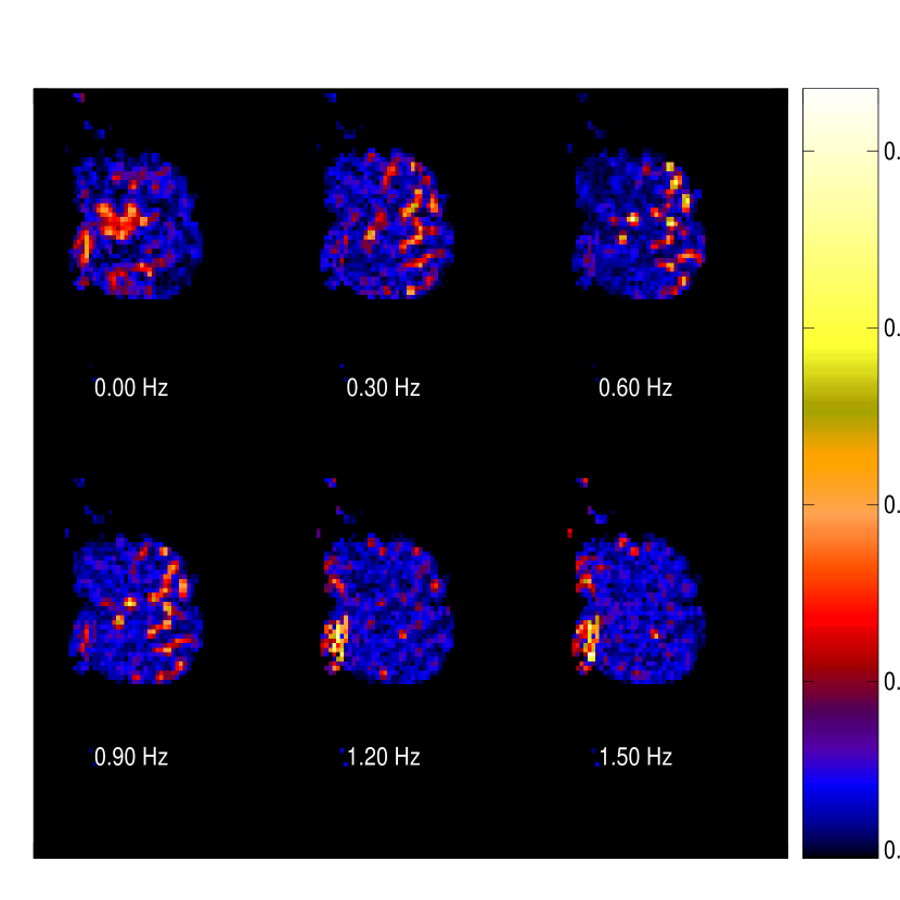
Figure 11: Amplitudes of leading spatial eigenmodes for the space-frequency SVD of fMRI datai from data set $\mathcal{C}$. Note that the spatial structure varies as a function of center frequency with the physiological oscillations segregating into distinct frequency bands.

4.3 Local Frequency Ensemble and Jackknife Error Bars

One important advantage of the multitaper method is that it offers a natural way of estimating error bars corresponding to most quantities obtained in time series analysis, even if one is dealing with an individual instance of a time series. The fundamental notion here is that of a local frequency ensemble. The idea is that if the spectrum of the process is locally flat over a bandwidth $2W$, then the tapered Fourier transforms $\tilde{x}_{k}(f)=\sum_{t=1}^{N}e^{-2\pi ift}x(t)w_{k}(t)$ constitute a statistical ensemble for the Fourier transform of the process at the frequency $f_{0}$. Assuming that the underlying process is locally white in the frequency range $[f_{0}-W,f_{0}+W]$, then it follows from the orthogonality of the data tapers that $\tilde{x}_{k}(f)$ are uncorrelated random variables with the same variance. For large N, $\tilde{x}_{k}(f)$ may be assumed to be asymptotically normally distributed under some general circumstances (For related results see [Mallows, 1967]). This provides one way of thinking about the direct multitaper estimate presented in the previous sections: the estimate consists of an average over the local frequency ensemble.

The above discussion serves as a motivation for multitaper estimates of the correlation function, the transfer function and the coherence between two time series. Given two time series $x_{t},y_{t}$, and the corresponding multiple tapered Fourier transforms $\tilde{x}_{k}(f),\tilde{y}_{k}(f)$, the following direct estimates can be defined [Thomson, 1982] for the correlation function $C_{yx}(f)=E[\tilde{y}(f)\tilde{x}^{*}(f)]$, the transfer function $T_{yx}(f)=E[\tilde{y}(f)\tilde{x}^{*}(f)]/E[|\tilde{x}(f)|^{2}]$ and the coherence function $\rho_{yx}(f)=E[\tilde{y}(f)\tilde{x}^{*}(f)]/\sqrt{E[|\tilde{x}(f)|^{2}]E[|\tilde{y}(f)|^{2}]}$:

$$\hat{C}_{yx}(f)={1\over K}\sum_{k=1}^{K}\tilde{y}_{k}(f)\tilde{x}_{k}^{*}(f)$$ (24)

$$\hat{T}_{yx}(f)={\sum_{k=1}^{K}\tilde{y}_{k}(f)\tilde{x}_{k}^{*}(f)\over\sum_{k=1}^{K}\tilde{x}_{k}(f)\tilde{x}_{k}^{*}(f)}$$ (25)

$$\hat{\rho}_{yx}(f)={\sum_{k=1}^{K}\tilde{y}_{k}(f)\tilde{x}_{k}^{*}(f)\over\sqrt{\sum_{k=1}^{K}|\tilde{x}_{k}(f)|^{2}\sum_{k=1}^{K}|\tilde{y}_{k}(f)|^{2}}}$$ (26)

Figure 12: Jackknife error bars on multitaper spectral estimate corresponding to spectrum shown in Fig. 6. The spectral estimate is the solid bar and the error bars are represented by dots.

These definitions allow the estimation of the coherence and transfer function from a single instance of a pair of time series. Using the local frequency ensemble, one can also estimate jackknife error bars for the spectra and the above quantities. The idea of the jackknife is to create different estimates by leaving out a data taper in turn. This creates a set of estimates from which an error bar may be computed [Thomson and Chave, 1991]. As an example, we show in Fig. 12 jackknife estimates of the standard deviations of the spectral estimate in Fig. 6.

5 Analysis techniques for different Modalities

We now deal with specific examples of data from different brain imaging modalities. We concentrate on general strategies for dealing with such data, and most of our techniques apply with minor changes across the modes. However, it is easier to treat the various cases seperately, and we present somewhat parallel developments in the following sections. The data sets $\mathcal{A}$ through $\mathcal{D}$ have been briefly discussed before.

5.1 Magnetoencephalography

In this section, we consider data set $\mathcal{A}$ consisting of multichannel MEG recordings. The number of channels is 74 (37 on each hemisphere), the digitization rate $2.083kHz$, and the duration of the recording is $5$ minutes.

5.1.1 Preprocessing

An occasional artifact in MEG recordings consists of regularly spaced spikes in the recordings due to cardiac activity. This is caused when the comparatively strong magnetic field due to currents in the heart are not well cancelled. To suppress this artifact, we proceed as follows: First, a space-time SVD is performed on the multichannel data. The cardiac artifacts are usually quite coherent in space, and show up in a few principal component time series. In those time series, the spikes are segmented out by determining a threshhold by eye and segmenting out 62.5ms before and after the threshhold crossing. The segmented heartbeat events are then averaged to determine a mean waveform. Since the heartbeat amplitude is not constant across events the heartbeat spikes are removed individually by fitting a scaling amplitude to the mean waveform using a least-squares technique. Each spike modelled by the mean waveform multiplied by a scaling amplitude is then subtracted from the time series. Fig.13 illustrates the results of this procedure.

Figure 13: Principal component time series of MEG data from data set $\mathcal{A}$ containing cardiac artifacts. The upper plot shows the time course before suppression and the spikes due to the heart beat are clearly visible. The lower plot shows the time course after suppression of the heart beat using the technique described in the text.

A fairly common problem in electrical recordings is the presence of $60Hz$ artifacts and on occasion sinusoidal artifacts at other frequencies. Such sinusoidal artifacts, if they lie in the relevant data range, are usually dealt with using notch filters. This is however unnecessarily severe since the notch filters may remove too large a band of frequencies, in particular in the case of MEG data where frequencies close to $60Hz$ are of interest. We find that the $60Hz$ line and other fixed sinusoidal artifacts can be efficiently estimated and removed using the methods for sinusoidal estimation described in section 4.1.5. Specifically, in this case the frequency of the line is accurately known (this requires a precise knowledge of the digitization rate) and one has to only estimate its amplitude and phase. This is done for a small time window using Eq.12. By sliding this time window along, one obtains a slowly varying estimate of the amplitude and phase, and is therefore able to reconstruct and subtract the sinusoidal artifact. The results of such a procedure are illustrated in Fig.14(a), where a time averaged spectrum is shown for a single channel before and after subtraction of the line frequency component. In Fig.14(b), the amplitude of the estimated 60Hz component is shown with its slow modulation over time.

$(a)$     $(b)$

Figure 14: a) Time averaged spectrum before and after subtraction of 60Hz artifact (single channel time series) from MEG data in data set $\mathcal{A}$. b) Estimated time varying amplitude of the 60 Hz line frequency.

5.1.2 Time Frequency Analysis

The spectral analysis of multichannel data presents the fundamental problem of how to simultaneously visualize or otherwise examine the time-frequency content of many channels. One way to reduce the dimensionality of the problem is to work with principal component time series. A space-time SVD of MEG data gives a rapidly decaying singular value spectrum. This indicates that one can consider only the first few temporal components to understand the spectral content of the data. For purposes of illustration of our techniques we consider the first three principal component time series in a 5 minute segment recording of spontaneous awake activity.

Figure 15: Autoregressive fit to averaged spectrum of MEG data from data set $\mathcal{A}$ averaged over non-overlapping windows in time for purposes of pre-whitening. The thick line shows the autoregressive fit to the average spectrum. The thin line shows the average spectrum. A low-order AR spectral estimate is used to reduce the dynamic range in the spectrum without fitting specific structural features of the data.

A useful preliminary step in spectral analysis is pre-whitening using an appropriate autoregressive model. This is necessary because the spectrum has a large dynamic range. Pre-whitening leads to equalization of power across frequencies, which allows better visualization of time-frequency spectra. In addition, a space-time SVD is better performed on pre-whitened data, since otherwise the large amplitude, low frequency oscillations completely dominate the principal components. The qualitative character of the average spectrum is a slope on a semilogarithmic scale (Fig.14(a)). The goal is to prewhiten with a low order AR model so that the peaks in the spectrum are left in place but the overall slope is removed. Considering the derivative of the spectrum rather than the spectrum itself achieves a similar result.

The procedure is to first calculate a moving estimate of the spectrum using a short time window ($T=0.35s$ in the present case) and a direct multitaper spectral estimator ($W=4/T;K=6$). These estimates are then averaged over time to obtain a smooth overall spectrum. Next, a low order autoregressive model (order $=10$ in the present case) is fit to the spectral estimate. We use the Levinson Durbin recursion to fit the AR model. Results of such a fit are shown in Fig.15. The coefficients of the autoregressive process are then used to filter the data, and the residuals are subjected to further analysis. Thus, if the coefficients obtained are $a_{k}$ and the original time series is $x_{t}$, then the residuals are $\delta x_{t}=x_{t}-\sum_{1}^{n}x_{t-k}a_{k}$ which are subjected to a time-frequency analysis.

Typical time frequency spectra of pre-whitened principal component time series are shown in Fig.16. The spectra were obtained using a direct multitaper estimate for $1s$ long time windows and for $W=4Hz,K=6$.

Figure 16: Time frequency spectrum of first three principal components obtained in a space-time SVD of MEG data from data set $\mathcal{A}$ pre-whitened by the filter shown in Figure 15.

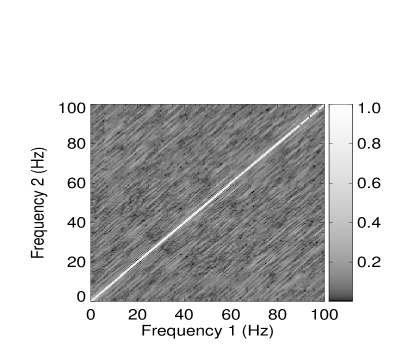
$(a)$     $(b)$

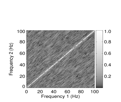
Figure 17: a) Magnitude of $\rho(f,f^{\prime})$ for the leading PC time series of MEG data from data set $\mathcal{A}$. b) Magnitude of $\rho(f,f^{\prime})$ for the leading PC time series after initially scrambling the time series.

To assess the quality of the spectral characterization it is important to quantify the presence (or absence) of correlations between fluctuations at different frequencies. One measure of the correlations between frequencies for a given time series is given by the following quantity analogous to the coherence between different channels:

$$\rho_{xx}(f,f^{\prime})={\sum_{k=1}^{K}\tilde{x}_{k}(f)\tilde{x}_{k}^{*}(f^{\prime})\over\sqrt{\sum_{k=1}^{K}|\tilde{x}_{k}(f)|^{2}\sum_{k=1}^{K}|\tilde{x}_{k}(f^{\prime})|^{2}}}$$ (27)

The estimate can be further averaged across time windows to increase the number of degrees of freedom. This quantity, computed for the leading principal component time series obtained earlier, is displayed in Fig.17(a). In this figure, the magnitude of the estimate $\rho(f,f^{\prime})$ for the leading PC time series is displayed as a function of the two arguments, $f$ and $f^{\prime}$. For comparison, in Fig.17(b), results of the same procedure obtained after initially scrambling the time series are also displayed. A visual comparison shows the lack of evidence for correlations across frequencies in an average sense.

Figure 18: Magnitudes of coherences for MEG from data set $\mathcal{A}$ between points in space displayed by lines of proportionate thickness. The coherences were computed for a center frequency of $20Hz$ and half bandwidth $5Hz$.

5.1.3 Multichannel Spectral Analysis

The time frequency spectra of leading principal components shown in the earlier section capture the spectral content of the MEG signal that is coherent in space. Alternatively, one can perform a space-frequency SVD with a moving time window on the data. It is also desirable to obtain time averaged characterizations of the coherence across channels. This can be done by considering the coherence functions between channels $\rho_{ij}(f)$, which can be estimated as in Eq.26 using multitaper methods. The estimate, when calculated for a moving time window, can be further averaged across time windows. Displaying the matrix $\rho_{ij}$ poses a visualization problem, since the indices $i,j$ themselves correspond to locations on a two dimensional grid. Thus, an image displaying the matrix $\rho_{ij}$ does not preserve the spatial relationships between channels. One solution to this visualization problem is presented in Fig.18, by representing the strength of the coherence between two space points by the thickness of a bond connecting the two points. This figure shows the coherence $\rho_{ij}(f)$ computed with a center frequency $20Hz$ and half bandwidth $5Hz$. The bond strengths have been threshholded to facilitate the display. This visualization, although not quantitative, allows for an assessment of the organization of the coherences in space.

Figure 19: Dominant spatial eigenmodes of a space-time SVD of band pass filtered MEG data from data set $\mathcal{A}$ for the frequency band 35-45 Hz. The two hemispheres of the brain are projected onto a plane, each being sampled by 37 sensors.

An alternative way of performing principal component analysis on space-time data while localizing information in the frequency domain is clearly to apply a space-time SVD to data which has first been frequency filtered into the desired band. To obtain frequency filters with optimal bandlimiting properties, projection filters based on DPSS are used. For illustration, we perform this analysis on the data under discussion. The individual channels were first filtered into the frequency band $35-45Hz$. This gives a complex time series at each spatial location. The first three dominant spatial eigenmodes in a space-frequency SVD are displayed in Fig. 19, with singular values decreasing from the top to the bottom of the figure. Since the spatial eigenmodes are complex, their values are represented by arrows, whose lengths correspond to magnitudes and whose directions correspond to phases. It is quite clear from the figure that the data shows a high degree of spatial coherence on an average.

5.2 Optical Imaging

In this subsection we consider optical imaging data. We consider the general case of imaging data gathered either using intrinsic or extrinsic contrast. The case of intrinsic contrast is closely related to fMRI, and the analysis parallels that of the fMRI data sets $\mathcal{C}$ and $\mathcal{D}$. To illustrate some effects important in the case of extrinsic contrast, we consider data set $\mathcal{B}$. Data set $\mathcal{B}$ was gathered in presence of a voltage sensitive dye, and consists of images of a isolated pro-cerebral lobe of Limax, with a digitization rate $75Hz$ and duration $23s$.

5.2.1 Spectral Analysis of PC Time Series

The general procedure outlined above for fMRI data consisting of a space-time SVD followed by a spectral analysis of the principal component (PC) time series is useful to obtain a preliminary characterization of the data. In particular, in the case of optical imaging data using intrinsic or extrinsic contrast in the presence of respiratory and cardiac artifacts, this procedure helps the assessment of the artifactual content of the data. However, as discussed earlier, the space-time SVD mixes up distinct dynamic components of the image data, and is therefore of limited utility for a full characterization of the data.

5.2.2 Removal of Physiological Artifacts

We have developed a method for efficient suppression of respiratory and cardiac artifacts from brain imaging data (including optical images and MRI images for high digitization rates) by modelling these processes by slowly amplitude and frequency modulated sinusoids. Other approaches to suppression of these artifacts in the literature include ‘gating’, frequency filtering, modelling of the oscillations by a periodic function [Le and Hu, 1996], and removal of selected components in a space-time SVD [Orbach et al., 1995]. These approaches have varying efficacies. For example, gating aliases the relevant oscillations down to zero frequency, so that any variation in these oscillations cause slow fluctuations in the data, which is in general undesirable. Frequency filtering removes more spectral energy than is strictly necessary from the signal. Modelling of the oscillations by a periodic function is imperfect because the oscillations themselves may vary in time. This can be rectified by allowing the parameters of the oscillations to slowly change in time. One must be able to fit a sinusoidal model robustly to short time series segments to do this properly. Finally, removing selected components in a space-time SVD is not a safe procedure, since, as discussed before, the space-time SVD does not necessarily separate the different components of the image data.

Our method for suppressing the above mentioned oscillatory components is based on multitaper methods for estimating sinusoids in a colored background described earlier. The method is based on modelling the oscillations by a sum of sinusoids whose amplitude and frequency are allowed to vary slowly. The modeled oscillations are removed from the time series in the data to obtain the desired residuals. Although a space-time SVD is not sufficient by itself, applying such a removal technique to the leading temporal principal components, and reconstituting the residual time series appears to give good results. This procedure was found to be effective for a wide variety of data, including optical imaging using both intrinsic and extrinsic contrast in rat brain, and in fMRI data. The details of the technique are presented in the section on fMRI data, section 5.3.

5.2.3 Space-Frequency SVD

Figure 20: Coherence spectrum for a space-frequency SVD of optical imaging data in data set $\mathcal{B}$ from the PC lobe of Limax.

In this section we present the results of a space-frequency SVD applied to data set $\mathcal{B}$. This technique has been described above (Fig.10 and 11) for data set $\mathcal{D}$. In Fig 20, the coherence spectrum is shown for data set $\mathcal{B}$. The coherence was computed on a coarse grid, since there is not much finer structure than that displayed in the spectrum. In this case, 13 DPSS were used, corresponding to a full bandwidth of $0.3Hz$. The preparation (pro-cerebral lobe of Limax) is known to show oscillations, which are organized in space as a traveling wave. Traveling waves in the image, gathered in the presence of a voltage sensitive dye, reflect traveling waves in the electrical activity. The coherence spectrum displayed in Fig.20 shows a fundamental frequency of about 1.25Hz and the corresponding first two harmonics.

The amplitudes of the leading spatial eigenmode as a function of center frequency are shown in Fig.21. Note that the spatial distribution of coherence is more localized to the center of the image at the higher harmonics. This reflects the change in shape of the waveform of oscillation that is known to occur in the preparation as a function of spatial position. This phenomenon has been interpreted as a result of differing spatial concentration profiles of two different cell types in this system [Kleinfeld et al., 1994]. Based on this past interpretation, the leading modes at the fundamental and harmonic frequencies directly reflect the spatial distribution of the different cell types.

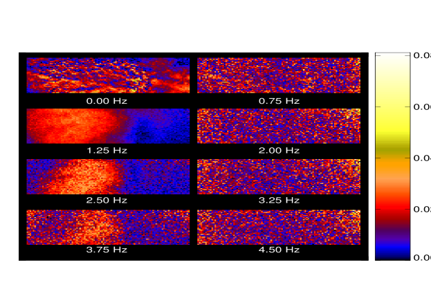
Figure 21: Leading spatial eigenmodes of the space-frequency SVD corresponding to Fig. 20. The amplitudes of the leading modes are shown as a function of center frequency.

$(a)$     $(b)$

Figure 22: Leading spatial eigenmodes of the space-frequency SVD corresponding to Fig.21. a) Gradients of the phase of the leading SVD mode at a center frequency of 2.5Hz, corresponding to local wave-vectors for the wave motion, are shown as arrows. These are superposed on constant phase contours for the mode. b) Constant phase contours for spatial eigenmodes of the space-frequency SVD for center frequencies 1.25 Hz and 2.5 Hz. 2.5 Hz is shown by the bold contour.

The spatial eigenmodes are complex, and possess a phase in addition to an amplitude. This allows for the investigation of traveling waves in the data. Let the leading spatial eigenmode, as a function of frequency, be expressed as

$$\tilde{I}_{1}(x;f)=A(x;f)e^{i\theta(x;f)}$$ (28)

Given the convention we are following for the Fourier transform (Eq.1), one may define the following local wave vector:

$${\bf k}(x;f)=-\mbox{\boldmath$\nabla$}\theta(x;f)$$ (29)

If the coherent fluctuations at a given frequency correspond to traveling plane waves, then ${\bf k}(x;f)$ corresponds to the usual definition of the wave vector. More generally, this quantity allows the systematic examination of phase gradients in the system, which corresponds to traveling excitations.

The local wavevector map for data set $\mathcal{B}$ at a center frequency of 2.5 Hz (the first harmonic) is shown in Fig.22(a), superposed on top of contours of constant phase. In Fig.22(b), the constant phase contours for center frequencies 1.25Hz, 2.5Hz (fundamental and first harmonic) are superposed. On superposing the contours for the fundamental and the first harmonic, we discover an effect that was not evident in the earlier analysis of the data [Kleinfeld et al., 1994], namely that the phase gradients at 1.25Hz and 2.5Hz are slightly tilted with respect to each other. This can be interpreted as two different waves simultaneously present in the system, but running in slightly different directions. Coexisting waves present at different temporal frequencies with different directions of propagation have also been revealed by space-frequency SVD analysis of voltage-sensitive dye images of turtle visual cortex [Prechtl et al., 1997].

5.3 Magnetic Resonance Imaging

The data sets $\mathcal{C}$ and $\mathcal{D}$ comprising functional MRI data have been used in earlier sections to illustrate the techniques presented in the paper (Figures 8-11). In this section, we continue to illustrate analytical techniques on this data set. The data sets were gathered with a digitization rate of $5Hz$ and a total duration of $110s$. Data set $\mathcal{C}$/$\mathcal{D}$ was gathered in the presence/absence of a flashing LED checkerboard pattern serving as visual stimulus. An extra problem in the analysis of MRI data is the presence of motion related artifacts, which have to be suppressed [Mitra et al., 1997].

5.3.1 Removal of Physiological Artifacts

Here a detailed description is provided of the method for removal of physiological oscillations discussed in the section on optical imaging data. A space-time SVD of the data is first computed, followed by sinusoidal modelling of the leading principal component time series. This is necessary for two reasons: (i) The images in question typically have many pixels, and it is impractical to perform the analysis separately on all pixels. (ii) The leading SVD modes capture a large degree of global coherence in the oscillations.

Consider a single principal component time series, $a(t)$. We assume that the time series is a sum of two components. The first component consists of a sum of amplitude and frequency modulated sinusoids representing respiratory and cardiac oscillations. The second component $\delta a(t)$ contains the desired signal.

$$a(t)=\sum_{n}A_{n}(t)\cos\bigl{(}f_{n}(t)t+\phi_{n}(t)\bigr{)}+\delta a(t)$$ (30)

The goal is to estimate the smooth functions $A_{n}(t),f_{n}(t)$ and $\phi_{n}(t)$, which give the component to be subtracted from the original time series.

It is necessary to choose an optimally sized analysis window. This window must be sufficiently small to capture the variations in the amplitude, frequency and phase, but must be long enough to have the frequency resolution to separate the relevant peaks in the spectrum, both artifactual and originating in the desired signal. The choice of window size depends to some extent on the nature of the data, and cannot be easily automated. However, in similar experiments it is safe to use the same parameters. Ideally, one would choose the window size in some adaptive manner, but we find it adequate for our present purposes to work with a fixed window size.

The frequencies $f_{n}(t)$ have to satisfy several criteria. Usually one is removing the respiratory and cardiac components. The corresponding spectra contain small integer multiples of two fundamental frequencies, with the possible presence of sidebands due to nonlinear interactions between the oscillations. The frequency F-test described in section 4.1.5 is used to determine the fundamental frequency tracks $f_{n}(t)$ in Eq.30. The time series used for this purpose may either be a principal component time series, or an independently monitored physiological time series. Note that the assumption here is that within an analysis bandwidth of the relevant peak in the cardiac or respiratory cycle, the data can be modeled as a sine wave in a locally white background. The fundamental frequency tracks are used to construct the tracks for the harmonics and the sidebands.

Figure 23: Time frequency plot of frequency tracks for a moving sinusoidal model of the cardiac and respiratory artifacts in fMRI data from data set $\mathcal{C}$. The analysis is performed on a principal component time series obtained by performing a space-time SVD.

Figure 24: Upper: Part of principal component time series forming the basis of Fig.23. Middle: Estimated cardiac and respiratory components corresponding to Upper plot. Lower: Time series with cardiac and respiratory components suppressed.

In the example, we show the results of the analysis on one principal component time series from data set $\mathcal{C}$. The fundamental frequency tracks were determined by using the F-test on a moving analysis window on the PC time series.

If the F-test does not provide a frequency estimate for short segments of the data, estimates may be interpolated using a spline, for example. After the frequency tracks are determined, the amplitude and phase of the sinusoids are calculated using Eq.12 for each analysis window location. Note that the shift in time between two successive analysis windows can be as small as the digitization rate of the data, but is limited in practice by the available computational resources. The estimated sinusoids are reconstructed for each analysis window, and the successive estimates are overlap-added to provide the final model waveform for the artifacts.

The frequency tracks are shown in Fig.23 superposed on a time-frequency spectral estimate of the principal component time series. In Fig.24, results of the procedure described above are shown in the time domain for the chosen principal component. Notice the change in the frequency corresponding to the cardiac cycle (around 1.3Hz) in the initial part of the time period. This would prevent the adequate estimation of this component if a model with fixed periodicity was used. In contrast the method used here allows for slow variations in the amplitudes of the oscillations in addition to variations in frequency. A strong stimulus response is noticeable in this principal component (data set $\mathcal{C}$ was gathered in presence of visual stimulus).

5.3.2 Space-Frequency SVD

Figure 25: Coherence spectrum for a space-frequency SVD of fMRI data from data sets $\mathcal{C}$ and $\mathcal{D}$ in presence of visual stimulus (solid curve) compared with absence of visual stimulus (dotted curve).

In this section, the results of a space-frequency SVD are shown for data sets $\mathcal{C}$ and $\mathcal{D}$. Recall that data sets $\mathcal{C}$ and $\mathcal{D}$ were collected with identical protocols, except that in data set $\mathcal{C}$ a controlled visual stimulus is applied. Fig.25 shows the coherence spectra resulting from the space-frequency SVD. In this calculation, the DPSS used corresponded to a full bandwidth of $0.1Hz$. The coherence spectra for the two data sets are more or less the same. The coherence near zero frequency is higher for data set $\mathcal{C}$  which contains the visual stimulus. The stimulus response can be seen clearly in the amplitude of the leading spatial eigenmode of the space-frequency SVD for data set $\mathcal{C}$ (Fig.26) at close to zero frequency. At higher frequencies, coherence arising from artifactual (respiratory) sources causes a different pattern of spatial amplitudes. As opposed to the space-time SVD, this procedure segregates the stimulus response from the oscillatory artifacts.

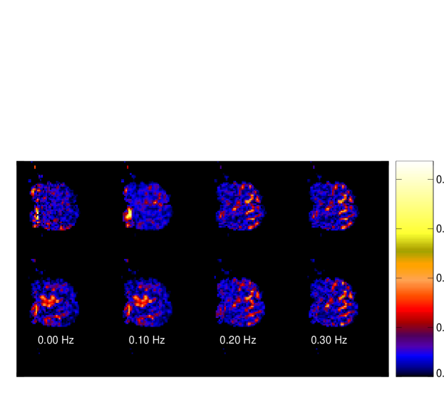
Figure 26: Amplitudes of leading spatial eigenmodes corresponding to the space-frequency SVD in Fig.25. Center frequencies from $0$ Hz to $0.3$ Hz in $0.1$ Hz increments. Upper: Without stimulus. Lower: With stimulus.

6 Discussion

We have tried to outline analysis protocols for data from the different modalities of brain imaging. It is useful recapitulate the essential features of these protocols in a unified manner, and to indicate the domains of validity of the different techniques proposed.

Visualization of raw data:
It is usually necessary to directly visualize the raw data, both as a crude check on the quality of the experiment, and to direct further analysis. In this stage, one may look at individual time series from the images, or look at the data displayed dynamically as a movie. The relevant images are often noisy, so that a noise reduction step is first necessary even before the preliminary visualization. In cases where the visualization is limited by large shot noise, truncation of a space-time SVD with possibly some additional smoothing provides a simple noise reduction step for the visualization.

Preliminary characterization:
In the next stage, it is useful to obtain quantities that help parse out the content of the data, in particular to identify the various artifacts. Despite its limitations, a space-time SVD is useful at this stage to reduce the data to a few time series and corresponding eigenimages. Examination of the aggregate spectra of the PC time series, for example, reveals the extent of cardiac/respiratory content of fMRI/optical imaging data. In case of MEG, direct examination of the PC time series reveals the degree of cardiac contamination. Examination of the corresponding spatial images reveals the spatial locations of the artifacts. In case of fMRI data, where the digitization rate may not be very high, studying the spectra can reveal whether cardiac/respiratory artifacts still lead to possibly aliased frequency peaks in the power spectra.

A further, more powerful characterization is obtained by the space-frequency SVD. For optical data and for rapidly sampled fMRI data, there is sufficient frequency resolution that at this stage the oscillatory artifacts segregate well. Studying the overall coherence spectrum reveals the degree to which the images are dominated by the respective artifacts at the artifact frequencies, while the corresponding leading eigenimages show the spatial distribution of these artifacts more cleanly compared to the space-time SVD. Moreover, provided the stimulus response does not completely overlap the artifact frequencies, a characterization is also obtained of the spatio-temporal distribution of the stimulus response. In case of fMRI, if the digitization rates are too slow (say less than 0.3Hz), there may not be any segregation in the frequency domain of the various components of the image; this can be established at this stage by examining the eigenimages of the space-frequency SVD. In this case, the techniques described in this paper would be of limited use.

Artifact removal:
Based on the preliminary inspection stage, one can proceed to remove the various artifacts to the extent possible. The techniques described in this paper are most relevant to artifacts that are sufficiently periodic, such as cardiac/respiratory artifacts in optical/fMRI data, 60 cycle noise in optical data/MEG, other frequency-localized noise such as building/fan vibrations (optical imaging data). There are two basic ways of using the frequency segregation of the artifacts to remove them. One method is to directly model the waveforms of the oscillations using the frequency and amplitude modulated sinusoidal fit described in the sections on optical/fMRI data.

For fMRI data, if the digitization rate is too low, then the techniques described here are not useful. However, for fMRI data, even with digitization rates of 1-2 seconds, it appears possible to use the frequency segregation of the physiological artifacts, using one of two methods. If auxiliary time series are available for cardiac/respiratory oscillations, one may construct the transfer function from these time series to the data using the multitaper technique described above, perform a statistical test of significance such as the F-test, and remove the significantly fitted components. Alternatively, if no auxiliary data are available, the space-frequency SVD may be examined for presence of these artifacts, and if the artifacts can be identified with some frequency band then filtering techniques may be used.

In each of the cases described above, the fundamental operation is performed on an individual time series. This may be performed pixel by pixel in the image, or to reduce computational time, the steps may alternatively be performed on the leading PC time series and the artifacts thus reconstructed may be then subtracted from the raw data.

Stimulus response characterization:
This is may be the most delicate step, since the goal of the experiment is usually to find the stimulus response which is not known a priori. If the stimulus is presented periodically and repeatedly, the transfer function may be computed in the frequency domain using the techniques described before. Often, some strong assumption is made about the stimulus response (e.g. the image intensity will rise during the stimulus), and methods of signal detection theory or statistical hypothesis testing are applied to extract the response based on the assumed signal model.

One general assumption about the stimulus response to a single trial might be that it lives in a particular region of frequency space. In the case of fMRI data, where the response is often a prolonged increase in signal intensity, this would correspond to the signal having relatively low frequencies. In this case, the space-frequency SVD described in the paper is of utility in describing the stimulus response, as illustrated in the section on fMRI data. Similarly, in optical imaging, if the stimulus was modulated with a particular temporal frequency, the same idea would be applicable.

It is to be emphasized that it is not possible to develop ”black box” like techniques which are a panacea to all problems of data analysis. It is neither possible nor desirable to entirely eliminate the human component in the process. However, relevant computational and analytical tools can be a powerful aid to making sense of the data, and are used most effectively in a closed loop system where the results of analysis influence experimentation.

References

- [Akaike, 1974] Akaike, H. (1974). A new look at the statistical model identification. IEEE Trans. Auto. Cont., 19:716–722.
- [Blasdel and Salama, 1986] Blasdel, G. and Salama, G. (1986). Voltage sensitive dyes reveal a modular organization in monkey striate cortex. Nature, 321:579–585.
- [Cleveland, 1993] Cleveland, W. S. (1993). Visualizing data. Hobart Press.
- [Davila et al., 1973] Davila, H., Salzberg, B., Cohen, L., and Waggoner, A. (1973). A large change in axon fluorescence that provides a promising method for measuring membrane potential. Nature, New. Biol., 241:159–160.
- [Denby and Mallows, 1991] Denby, L. and Mallows, C. L. (1991). Singular values of large matrices subject to gaussian perturbations. In Computing Science and Statistics: Proceedings of the 23rd Symposium on the Interface, pages 54–57. Interface Foundation.
- [Denk et al., 1990] Denk, W., Strickler, J., and Webb, W. (1990). Two photon laser scanning fluorescence microscopy. Science, 248:73–76.
- [Duda and Hart, 1973] Duda, R. O. and Hart, P. E. (1973). Pattern Classification and Scene Analysis. Wiley.
- [Grinvald et al., 1992] Grinvald, A., Lieke, E., Frostig, R., Gilbert, C., and Wiesel, T. (1992). Functional architecture of cortex revealed by optical imaging of intrinsic signals. Nature, 324:361–364.
- [Hamalainen et al., 1993] Hamalainen, M., Hari, R., Ilmonieni, R., Knuutila, J., and Lounasmaa, O. (1993). Magnetoencephalography - theory, instrumentation, and applications to noninvasive studies of the working brain. Rev. Mod. Phys., 65(2):413–497.
- [Joliot et al., 1994] Joliot, M., Ribary, L., and Llinas, R. (1994). Human oscillatory brain activity near 40 hz coexists with cognitive temporal binding. Proc. Natl. Acad. Sci., 91(24):11748–11751.
- [Kleinfeld et al., 1994] Kleinfeld, D., Delaney, K., Fee, M., Flores, J., Tank, D., and Gelperin, A. (1994). Dynamics of propagating waves in the olfactory network of a terrestrial mollusk - an electrical and optical study. J. Neurophys., 72(3):1402–1419.
- [Kwong et al., 1992] Kwong, K., Belliveau, J., Chesler, D., Goldberg, I., Weiskoff, R., Poncelet, B., Kennedy, D., Hoppel, B., Cohen, M., and Turner, R. (1992). Dynamic mabgetic resonance imaging of human brain activity during sensory stimulation. Proc. Natl. Acad. Sci., 89:5675–5679.
- [Le and Hu, 1996] Le, T. H. and Hu, X. P. (1996). Retrospective estimation and correction of physiological artifacts in fmri by direct extraction. Mag. Res. Med., 35(3):290–298.
- [Mallows, 1967] Mallows, C. (1967). Linear processes are almost gaussian. J. Appl. Prob., 4:313–329.
- [Mann and Park, 1994] Mann, M. E. and Park, J. (1994). Global-scale modes of surface temperature. J. Geophys. Res. Atmos., 99(D12):25819–25833.
- [Mayhew et al., 1996] Mayhew, J., Askew, S., Zheng, Y., Porrill, J., Westby, G., Redgrave, P., Rector, D., and Harper, R. (1996). Cerebral vasomotion: 0.1hz oscillation in reflected light imaging of neural activity. Neuroimage, 4(3):183–193.
- [Mitra et al., 1997] Mitra, P. P., Ogawa, S., Hu, X. P., and Ugurbil, K. (1997). The nature of spatiotemporal changes in cerebral hemodynamics as manifested in functional magnetic resonance imaging. Mag. Res. Med., 37(4):511–518.
- [Ogawa et al., 1992] Ogawa, S., Tank, D., Menon, R., Ellerman, J., Kim, S., Merkle, H., and Ugurbil, K. (1992). Intrinsic signal changes accompnaying sensory stimulation - functional mapping with magnetic resonance imaging. Proc. Natl. Acad. Sci., 89(13):5951–5955.
- [Orbach et al., 1995] Orbach, D., Obrien, E. V., Everson, R., Kaplan, E., Knight, B., and Sirovich, L. (1995). Time-course and wavelength dependence of the intrinsic optical signal in visual cortex investigated with a modified karhunen-loeve procedure,. Invest. Opth. Vis. Sci., 36(4):S873.
- [Pawley, 1995] Pawley, J. (1995). Handbook of Biological Confocal Mocroscopy. Plenum Press, N.Y. and London.
- [Percival and Walden, 1993] Percival, D. B. and Walden, W. T. (1993). Spectral analysis for physical applications : multitaper and conventional univariate techniques. Cambridge University Press.
- [Prechtl et al., 1997] Prechtl, J., Cohen, L. B., Pesaran, B., Mitra, P. P., and Kleinfeld, D. (1997). Visual stimuli induce waves of electrical activity in turtle cortex. Proc. Natl. Acad. Sci., 94(14):7621–7626.
- [Rapp et al., 1994] Rapp, P. E., Albano, A. M., Zimmerman, and I. D., Mimenez, M. (1994). Phase-randomized surrogates can produce spurious identifications of nonrandom structure. Phys. Lett. A, 192(1):27–33.
- [Slepian and Pollak, 1961] Slepian, D. and Pollak, H. O. (1961). Prolate spheriodal wavefunctions fourier analysis and uncertainty i. Bell Sys. Tech. Journal, 40:43–63.
- [Theiler and Rapp, 1996] Theiler, J. and Rapp, P. E. (1996). Reexamination of the evidence for low-dimensional, nonlinear structure in the human electroencephalogram. EEG Clin. Neurophys., 98(3):213–222.
- [Thomson, 1982] Thomson, D. J. (1982). Spectrum estimation and harmonic analysis. Proc. IEEE, 70(9):1055–1096.
- [Thomson, 1990] Thomson, D. J. (1990). Time series analysis of holocene climate data. Phil. Trans. Roy. Soc. Lond. A, 330:601–616.
- [Thomson and Chave, 1991] Thomson, D. J. and Chave, A. D. (1991). Advances in Spectrum Analysis and Array Processing, volume 1, chapter Jackknifed Error Estimates for Spectra, Coherences, and Transfer Functions, pages 58–113. Prentice Hall.
- [Welch, 1967] Welch, P. D. (1967). The use of fast fourier transform for the estimation of power spectra: A method based on time averaging over short, modified periodograms. IEEE Trans. Aud. Electro., 15:70–73.