Measuring the dynamics of neural responses in primary auditory cortex
Didier A.Depireux, Jonathan Z. Simon and Shihab A.Shamma

Electrical Engineering Department & Institute for Systems Research
University of Maryland
College Park MD 20742–3311, USA
(301) 405-6842

We review recent developments in the measurement of the dynamics of the response properties of auditory cortical neurons to broadband sounds, which is closely related to the perception of timbre. The emphasis is on a method that characterizes the spectro-temporal properties of single neurons to dynamic, broadband sounds, akin to the drifting gratings used in vision. The method treats the spectral and temporal aspects of the response on an equal footing.

Keywords: Auditory cortex, Spatial frequency, Temporal frequency, Separability, Ripples

1 Introduction

1.1 Timbre

We classify everyday natural sounds by their loudness (related to the intensity of the sound), their pitch (the perceived tonal height) and their timbre (the quality of the sound; that which is neither loudness nor pitch). The perception of timbre, which will be the main focus of this paper, is what allows us to tell the difference between two vowels spoken with the same pitch, or the difference between a clarinet and an oboe playing the same note. When hearing several musical instruments simultaneously, we can usually tell which instruments are playing by identifying the different timbres present in the mixed sound. Additionally, the perception of timbre is quite robust in the presence of noise and echoes (or reverberations), or even severe degradation such as during a telephone conversation, in which the sound is severely band-passed. Timbre perception is therefore an essential attribute of our sense of hearing.

To understand how we extract these different aspects of a sound, we must unravel what the auditory representation is along the neural pathway. The approach presented here takes the point of view that the principles used by neural systems are universal, once the stimulus has reached beyond the sensory epithelium (whether the cochlea’s basilar membrane or the retina). In particular the ideas presented here are frequently guided by considering the basilar membrane as a spatial axis, analogous to a one-dimensional retina, and then using the methods of visual gratings (drifting and otherwise), to study and characterize cells in the auditory cortex.

1.2 Auditory Cortex

A few general organizational features have long been recognized in Primary Auditory Cortex (AI), the location of which is shown in Figure 1. First is a spatially ordered tonotopic axis, along which cell responses are tuned from low to high frequencies¹; this is alternatively called a cochleotopic axis, which reflects the activity along the cochlea. Note that there are many fields in the auditory cortical area (the Anterior Auditory Field is shown in Figure 1), most of which display a tonotopic organization.

Figure 1: The position of the Primary Auditory Cortex (AI) in the ferret brain. The location of the Anterior Auditory Field (AAF) for illustration purposes. On the right the tonotopic axis is overlaid for both AI and AAF.

Second, perpendicular to the tonotopic axis, cells are arranged in alternating bands according to binaural properties: bands of cells are alternatively excited or inhibited by stimulation of the ipsilateral ear (the contralateral ear usually produces an excitatory response²). The tonotopic and binaural dominance organization is analogous to the retinotopic and ocular dominance columns of visual cortex. Other parameters have also been used to describe characteristics that change systematically along isofrequency lines. Using combinations of two pure tones, one can measure the Response Area (RA), also known as frequency-threshold curve, i.e. the response threshold of a cell as a function of the tone frequency presented. It has been shown that most RAs are topographically organized along the isofrequency lines according to the symmetry of their excitatory and inhibitory sidebands³. Other parameters have been also been shown to change systematically in cat, such as threshold⁴, bandwidth⁵ and frequency modulation direction selectivity^3,6.

These properties of AI cells are derived using pure tones (or clicks) akin to using dots of light (or flashes) to study cells in the visual pathway. Below we explain how to use the auditory version of drifting gratings⁷ to characterize response properties of cells to dynamic broadband sounds. This is necessary to gain insight to how timbre is encoded. Another advantage of the method presented here is that it allows us to determine the temporal and spectral properties of a cell at the same time. In particular, one can study whether and to what extent the response field varies as a function of time, thereby characterizing the cell with a full spectro-temporal response field.

2 Background

2.1 Response Field

Traditionally, cells along the auditory pathway have been characterized by their RA, or tuning curve. Determined using pure tones and by modifying the frequency of the stimulus while adjusting its intensity, the RA is the frequency-intensity combinations that elicit a threshold response, whether the sustained activity level or the strength of the onset response. In this paper, we use the Response Field (RF), a function measured using broadband sounds. As illustrated in Figure 2, it roughly reflects the range of frequencies that influence the discharge properties of the neuron under study. It is given in the form of a function, with positive values describing excitation (proportional to the RF’s amplitude) and negative values describing inhibition. In general, the RF is a spectro-temporal function, as opposed to the RA which typically describes only static properties (but see Nelken⁸ et al and Sutter⁹ et al). The definition of RF will be made more precise later.

Figure 2: Two idealized RFs at a given time. One RF (unbroken line) is centered on low frequencies and is asymmetric, and the other (broken line) is centered on high frequencies and is symmetric.

2.2 Natural Sounds

Natural sounds, such as environmental sounds, music and speech, are classified along several perceptual axes. We typically describe a sound by its loudness, its pitch and its timbre. Pitch is what changes when we pronounce the same vowel with different tonal heights, e.g. the pitch of a female voice is typically higher than the pitch of a male voice. Timbre is what changes when, keeping the same tonal height, we pronounce different vowels (e.g. /ah/, /eh/, /ih/). Figure 3 illustrates the spectral profile or envelope of a sound. The envelope of a sound can be viewed as a low-order polynomial fit of the (time-windowed) spectrum of the sound. A common method for the extraction of the envelope is the Linear Predictive Method (LPC)¹⁰; we will not go into the details of LPC here, instead referring the reader to the intuitive notion of envelope illustrated in Figure 3.

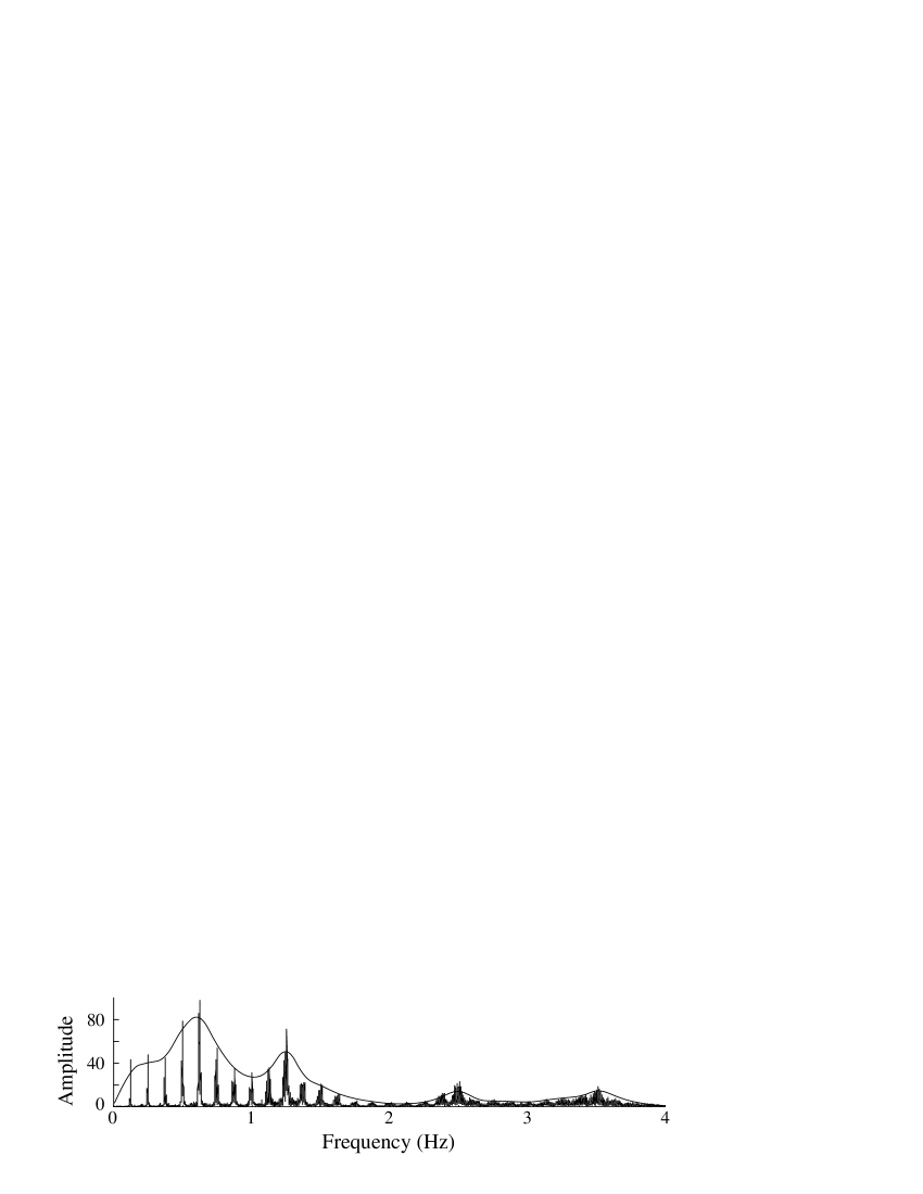
Figure 3: The spectrum of /aa/ spoken by one of the authors, with the spectral envelope superimposed on it.

The percept of timbre has been typically ascribed to the extraction of the envelope of the spectrum, but it also includes the temporal variations in the spectral envelope (for instance, the sound of a piano note played backwards sounds more like that of a wind organ, even though the amplitude of the Fourier transform of a sound and its time-reversed version are identical). Therefore, the study of how timbre is encoded must include temporal as well as spectral properties of the system. For speech, the temporal variations in timbre involve time-scales of about 10 Hz, so that this dimension of time is different from the temporal frequencies that make up sounds. It is the extraction of the dynamic spectral envelope by the auditory cortex that we are concerned with. Because we are interested in timbre, we use pitchless, dynamic, broadband sounds as stimuli.

2.3 Auditory Pathway (Monaural)

The auditory pathway up to primary auditory cortex, ignoring structures usually considered dedicated to binaural aspects of sounds (such as localization) can be minimally described as follows. The vibrations of the tympanic membrane are mechanically transformed into a traveling wave in the cochlea, with a profile that depends on the frequency content of the acoustic spectrum. The vibrations of the basilar membrane are transformed by inner hair cells into patterns of neural activity in the auditory nerve. For practical purposes, we can think of the basilar membrane as a collection of 1/3 octave filters, performing a time-windowed Fourier transform, with a time characteristic of about 30 ms. The auditory nerve projects to the Cochlear Nucleus, which contains a variety of cells with different properties. These cells project to the Lateral Lemniscus, then to the Inferior Colliculus, then to the Medial Geniculate Body in the Thalamus, and finally to the Auditory Cortex. As with all other sensory modalities, there are strong back projections for most forward projections.

Neurons at different stages of the auditory pathway respond to different time-scales. Neurons in the mammalian auditory nerve phase-lock to a pure tone up to frequencies of about 4 kHz: that is, they tend to fire at a specific phase of the tonal input, even if they fire in a sustained fashion at the maximum rate of about 200 spikes/second.¹¹ In the cochlear nucleus certain cells (so-called lockers) can phase-lock to tones for frequencies up to about 2 kHz.^12,13 By the Inferior Colliculus, most cells phase-lock to variations in the stimulus up to about 200 Hz with some cells going up to 800 Hz.^14,15 Finally, at the level of cortex, we have found that phase-locking to variations in the stimulus is usually on the order of 10 Hz with a maximum of about 70 Hz.¹⁶ Characterizing single units and their temporal features may ignore other potential coding strategies based on population activity. In the cat’s cochlea, 3000 inner hair cells innervate 50,000 auditory fibers,¹⁷ and by the auditory cortex, activity has been distributed over several millions of neurons.

Another important aspect of the organization of the auditory pathway is that cells tend to be organized in a tonotopic manner at each step: the frequency decomposition performed by the basilar membrane is along an axis which is logarithmic. Up through AI, cells that are equally spaced along a certain axis (which depends on the structure) respond best to sounds that are linearly spaced on a logarithmic frequency axis.

3 Principles

3.1 Guiding Principles

The guiding principle behind our research program is that cells behave like a linear system with respect to the spectral envelope. The proof of linearity is that when cells are presented with a sound made of up the sum of several spectral envelopes, the response, as measured assuming a rate code, is the sum of the responses to the individual envelopes. A response linear in frequency and time is characterized by a two-dimensional impulse response (or time-dependent response field) or equivalently, its Fourier transform, a two-dimensional transfer function. The extraction of this two-dimensional response field, a function of frequency and time, is the object of this paper.

It is helpful to remember that because the cochlea performs in some sense a time-windowed Fourier transform of the incoming waveform along its length, it is constructive to treat the frequency axis as a spatial axis, not the Fourier transform of the time axis. Since the frequencies are mapped logarithmically along the cochlear axis, the natural unit along the spectral axis is $x=\log(f)$. Much research on which the present work is based has dealt with the spectral, time-independent aspect of the response fields and linearity.¹⁸

3.2 Response Field and Linearity

Initially ignoring the dimension of time (or taking a delta function for the temporal impulse), the response of a cell with a response field $RF(x)$, to a sound with a spectral envelope $S(x)$, is given by $y=\smallint S(x)\cdot RF(x)dx$. Incorporating time (or allowing for more realistic temporal Impulse Response functions), we first limit our study to the case in which the temporal and spectral properties that characterize the cells’ responses are independent one from the other (separable). The response of a cell is then characterized by two functions, $RF(x)$, which describes the spectral properties, and $IR(t)$, which describes the temporal properties of the cell. Then, the response of a cell is described by $y(t)=\left({\smallint S(x,t)\cdot RF(x)\;dx}\right)*IR(t)$ where $*$ is the convolution operator. We will see that we can characterize certain cells in this way.

In the general situation, cells must be characterized by a full spectro-temporal description, i.e. a Spectro-Temporal Response Field, $STRF(x,t)$. In this case the response is given by $y(t)=\smallint S(x,t)*_{t}STRF(x,t)\;dx$, where the $*_{t}$ means convolution in the $t$ direction (with multiplication in the $x$ direction).

In the following, it is useful to consider the Fourier transform of the two-dimensional impulse response function, $STRF(-x,t)$, called the transfer function, $T\left({\Omega,w}\right)$, where we define $T\left({\Omega,w}\right)={\cal F}_{\Omega,w}\left[{STRF(-x,t)}\right]$. The coordinate dual to $x$ is $\Omega$, and the coordinate dual to $t$ is $w$.

3.3 Spectro-Temporal Response Field

Our general problem can be formulated as follows: $S(x,t)$ is the spectro-temporal envelope of the sound. Given the $STRF(x,t)$ of a neuron, we can measure its response to any $S(x,t)$. We obtain this $STRF$ from measurements of the neuron’s response to a complete set of basis functions $S_{\Omega w}\left({x,t}\right)$. A simple set of basis functions is $S_{\Omega w}(x,t)=\sin 2\pi(\Omega\cdot x+w\cdot t)$ where $S=0$ corresponds to a flat envelope of fixed loudness (i.e. noise). Any orthogonal basis will do, but the use of a sinusoidal basis allows us to use the standard methods of Fourier analysis. Furthermore, because of non-linearities discussed below, the sinusoidal basis is robust against distortion. We use the sinusoidal basis functions, and call them ‘ripples’. For this reason $\Omega$ is called ripple frequency (in cycles/octave) and w is called ripple velocity (in cycles/second, or Hertz).

Figure 4: Spectrotemporal envelope of a ripple, moving downward in frequency with $w$ = 3 Hz and $\Omega$ = 0.6 cycles/octave.

The most prominent non-linear distortions are half-wave rectification and compression. The half- wave rectification is due to the impossibility of negative spike rates (assuming the steady-state response to a flat spectrum to be zero, as will be seen to be the case); the distortion of a sinusoid due to firing rate half-wave rectification does not affect the phase of the response, and its effect on the amplitude of the first Fourier component is a constant factor (independent of $\Omega$ and $w$). The distortion due to compression does not affect the phase of the response.

3.4 Transfer Functions

By measuring the response $y_{\Omega w}\left(t\right)$ of a cell to a ripple of specific ripple frequency $\Omega$ and ripple velocity $w$, we can obtain the transfer function $T\left({\Omega,w}\right)$ at one point in $\Omega-w$ space.

$$y_{\Omega w}\left(t\right) =\int\!\!\!\int{dx^{\prime}dt^{\prime}\,STRF\left({x^{\prime},t^{\prime}}\right)\ \sin 2\pi\left({\Omega x^{\prime}+w\left({t-t^{\prime}}\right)}\right)}$$ (1)

$$=\Im\,\int\!\!\!\int{dx^{\prime}dt^{\prime}\;STRF(x^{\prime},t^{\prime}){\rm e}^{2j\pi\left({\Omega x^{\prime}+w\left({t-t^{\prime}}\right)}\right)}}$$

$$=\Im\left[{{\rm e}^{2j\pi wt}\int\!\!\!\int{dx^{\prime}dt^{\prime}\ }STRF(x^{\prime},t^{\prime}){\rm e}^{2j\pi\left({\Omega x^{\prime}-wt^{\prime}}\right)}}\right]$$

$$=\Im\left[{{\rm e}^{2j\pi wt}\,\,F_{\Omega,w}\left[{STRF\left({-x^{\prime},t^{\prime}}\right)}\right]}\right]$$

$$=\Im\left[{{\rm e}^{2j\pi wt}\,\,T\left({\Omega,w}\right)}\right]$$

$$=\Im\left[{{\rm e}^{2j\pi wt}\,\,\left|{T\left({\Omega,w}\right)}\right|{\rm e}^{j\Phi\left({\Omega,w}\right)}}\right]$$

$$=\left|{T\left({\Omega,w}\right)}\right|\ \sin\left[{2\pi wt+\Phi\left({\Omega,w}\right)}\right]$$

In this way, we derive the amplitude $\left|{T\left({\Omega,w}\right)}\right|$ and phase $\Phi\left({\Omega,w}\right)$ of the complex transfer function $T(\Omega,w)$ by measuring the amplitude and phase of the (real) response of the cell. By the definition of the transfer function, it follows that the inverse Fourier transform of $T(\Omega,w)$ is the STRF of the cell: $STRF(x,t)={\cal F}^{-1}{}_{-x,t}\left[T_{\Omega w}\right]$.

Because $STRF(x,t)$ is real, but $T(\Omega,w)$ is complex, there is a complex conjugate symmetry,

$$T\left({\Omega,w}\right)=T^{*}\left({-\Omega,-w}\right)$$ (2)

which holds for the Fourier transform of any real function of $x$ and $t$.

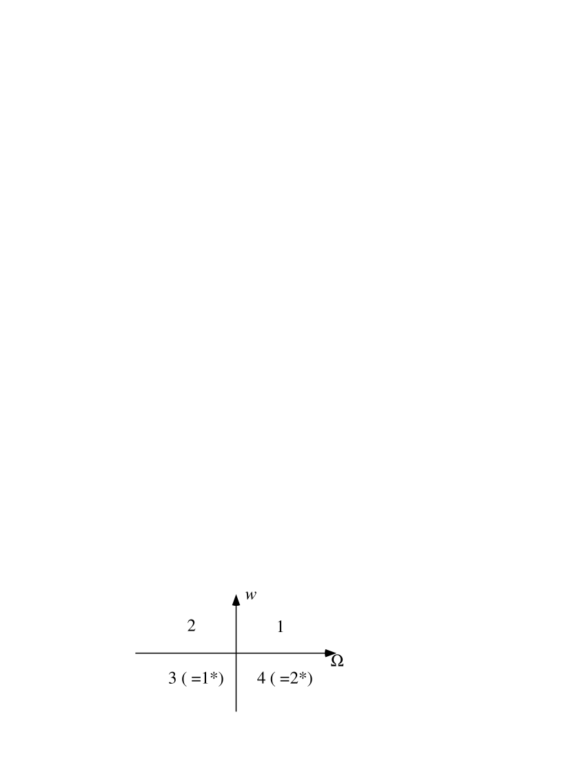
Figure 5: The $\Omega$ - $w$ plane. The value of the transfer function at a point in quadrant 1 is the complex conjugate of the value at the corresponding reflected point in quadrant 3 (and similarly for the quadrant pair 2 & 4). The ripple in Figure 4 corresponds to a pair of points in quadrants 1 and 3.

3.5 Full Separability

Many cells possess transfer functions that are fully separable, i.e. the ripple transfer function factorizes into a function of $\Omega$ and a function of $w$ over all quadrants: $T(\Omega,w)=F(\Omega)\cdot G(w)$. This implies that $STRF(x,t)$ is spectrum-time separable: $STRF(x,t)=RF(x)\cdot IR(t)$. In this case, we only need to measure the transfer function for all $\Omega$ at an arbitrary $w$, and for all $w$ at an arbitrary $\Omega$. Then $F(\Omega)$ and $G(w)$ are each complex-conjugate symmetric (because $RF(x)$ and $IR(t)$ are real), and we need only consider the positive values of each. This dramatically decreases the number of measurements needed to characterize the STRF.

3.6 Quadrant Separability

For cells that are not fully separable, we have found that they are still quadrant separable,¹⁶ i.e. the transfer function $T(\Omega,w)$ can be written as the product of two independent functions:

$$T\left({\Omega,w}\right)=\left\{\matrix{F_{1}\left(\Omega\right)\,G_{1}\left(w\right)&\Omega>0,w>0\hfill\cr F_{2}\left(\Omega\right)\,G_{2}\left(w\right)&\Omega<0,w>0\hfill\cr}\right.$$ (3)

where the subscript 1 indicates the $\Omega>0,w>0$ quadrant, and the subscript 2 the $\Omega<0,w>0$ quadrant. Note that by reality of the STRF, the transfer function in quadrants 3 ($\Omega<0,w<0$) and 4 is complex conjugate to quadrants 1 and 2 respectively. In this case, the STRF is not separable in spectrum and time, but is the linear superposition of two functions, one with support only in quadrant 1 (and 3), and one with support only in quadrant 2 (and 4).

3.7 Confirming Separability

Separability is measured by comparing the measured transfer function taken along parallel lines of constant $\Omega$ or constant $w$. If the sections of the transfer function differ only by a constant amplitude and phase factor, then that section is independent of the perpendicular variable and therefore the transfer function is separable. If in addition the section of the transfer function is complex-conjugate symmetric about zero, then the transfer function is fully separable. Otherwise the transfer function is merely quadrant-separable.

3.8 Confirming Linearity

The method we use to characterize cortical cells depends on their being linear, so linearity must be assessed. To this end, we measure (as described above) the transfer function of a cell with single ripples, and then measure the extent to which we can predict the response of the cell to a linear combination of ripples. Confirmation of linearity comes from measuring the response of the cell to linear combinations of ripples, thereby verifying the degree of linearity of the response.

Predicting the response of the cell to linear combinations of ripples for which the transfer function was not measured directly, but only inferred via separability, verifies both linearity and separability simultaneously.

3.9 Characterizing the Response

The functions $F(\Omega)$ and $G(w)$ are unconstrained theoretically. Physiologically, however, there are constraints on the type of functions they may be. For instance, because $F(\Omega)$ is the Fourier transform of $RF(x)$ which is localized around a center frequency ($f_{m}$ in frequency space, $x_{m}$ in logarithmic frequency space), the phases of $F(\Omega)$ must constructively interfere at $x_{m}$, and the amplitude of $F(\Omega)$ must be band limited. See, e.g. Figure 2 for examples of RFs, each of which is band limited and centered at a different $x_{m}$.

3.9.1 Amplitude of the response

The amplitude of the ripple frequency transfer function $F(\Omega)$ reaches a maximum at $\Omega_{m}\approx\left({2BW}\right)^{-1}$, where $BW$ is the excitatory bandwidth of the RF in octaves, and then decreases: at higher ripple frequencies the modulations of the ripple’s spectral envelope cancel when integrated against the (more slowly varying) RF; at ripple frequencies lower than $\Omega_{m}$, the energy in the ripple’s spectrum is fairly constant over the width of the RF, including any negative sidebands, and therefore integrates to a smaller magnitude. Similarly, the amplitude of the ripple velocity transfer function G(w) has a maximum at $w_{m}\approx\left({2BW_{t}}\right)^{-1}$, where $BW_{t}$ is the temporal excitatory width of the IR. Because under anesthesia the steady state response to any sound with a constant envelope has a rate of zero in cortex, we get $G(0)=\int{dt\,IR\left(t\right)}=0$.

3.9.2 Phase of the response

Because neurons in the auditory pathway are tonotopically arranged, each cell has a frequency around which the RF is centered which is independent of the ripple frequency $\Omega$. Since the derivative of the phase of $F(\Omega)$ gives the mean frequency of the response for that ripple frequency, the phase of the transfer function is linear (plus a constant). Similarly, because IR is causal, there is a group delay, and because of the biological nature of the neural process, the delay is roughly independent of ripple velocity, which gives a constant derivative of the phase of $G(w)$.

Therefore the phase of the transfer function $\Phi^{q}\left({\Omega,w}\right)$ (see Equation (1)), $q=\left\{{1,2}\right\}$ (for each quadrant), can be written as $\Phi^{q}\left({\Omega,w}\right)=2\pi\Omega x_{m}^{q}+2\pi w\tau_{d}^{q}+\chi^{q}$, where $x_{m}^{q}=\log f_{m}^{q}$ is the mean frequency around which the RF is centered, and $\tau_{d}^{q}$ is the delay of the IR, defined as the mean of the envelope of the IR.. $\chi^{q}$ is a constant phase angle. Tonotopy guarantees that $x_{m}^{1}\approx x_{m}^{2}$, but depending on the precise inputs of the neuron, they may not agree completely, so that we can have different $x_{m}$ for upward and downward moving sounds. Similarly, $\tau_{d}^{1}\approx\tau_{d}^{2}$, but equality is not required. The reality of the response enforces complex-conjugate symmetry of the transfer functions, allowing for these six independent parameters to describe the phase everywhere in the $\Omega--w$ plane. A convenient convention is to define constant phase angles $\theta$ and $\phi$ such that $\chi^{1}=\theta+\phi,\;\chi^{2}=\theta-\phi$. With the complex-conjugate symmetry, and if the STRF is separable, $\phi$ is the symmetry parameter of the RF and $\theta$ is the symmetry parameter of the IR (in Figure 2, $\phi=90^{o}$ for the left cell and $\phi=0^{o}$ for the right cell). Even in the non-separable case, we will still call $\phi$ the RF symmetry and $\theta$ the IR polarity. If one restricts measurements to one quadrant plus the $w$-axis (recall from above that the transfer function vanishes on the $\Omega$-axis), one can measure $\chi$ in that quadrant and, on the axis, the average of $\chi^{1}$ and $\chi^{2}$, i.e. $\theta$. There is an ambiguity in fixing $\theta$ and $\phi$ that allows us to restrict $\theta$ to lie between $0^{o}$ and $180^{o}$, while $\phi$ ranges the full $-180^{o}$ to $+180^{o}$.

Figure 6: The phase of the transfer function can be described by 6 parameters over most of the relevant regions of the $\Omega$ - $w$ plane.

The phase curve does not truly have a discontinuity across the axis. For very small ripple frequencies, the response becomes more independent of the best frequency of the cell, allowing the slope to change continuously from its constant value to $\theta$. At large ripple frequency the slope may also diverge from its constant value, but at these ripple frequencies the amplitude is small and so the particular values of the phase do not contribute. Similarly, the phase of $G(w)$ is constant over its intermediate range but changes continuously to $\phi$ on the $\Omega$-axis. Since the amplitude is zero on that axis, this is not so important.

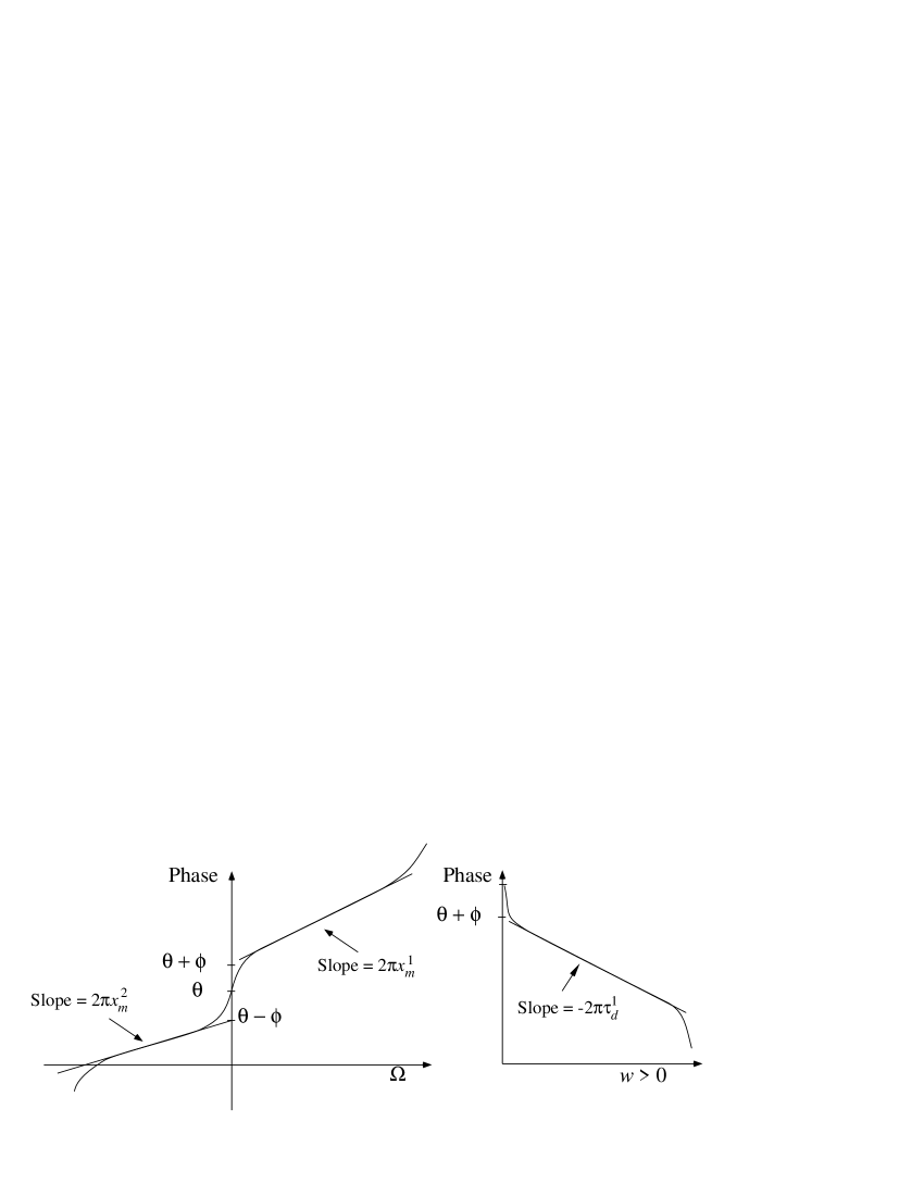
Figure 7: Phase Curves. The slope is constant for most of the curves, after (left) $2\pi w\tau_{d}^{q}$ has been removed from the corresponding quadrants, corresponding to a center frequency that is independent of the ripple frequency, and (right) after $2\pi\Omega x_{m}^{1}$ has been removed, corresponding to a delay that is independent of ripple velocity. At very small ripple frequencies (long ripple periodicity), center frequency is less meaningful, and similarly for small ripple velocity and delay, respectively. At large ripple velocity the slope asymptotes to the signal-front delay, but when this occurs the small amplitude of the transfer function makes it difficult to measure the phase (see Dong and Atick²¹ and Papoulis¹⁹).

4 Analytical Methods

4.1 The Ripple Stimulus

The auditory stimulus we use has a sinusoidal profile at any instant in time. Since it would be hard to generate noise and then shape it with filters, we generate ripples over a range of 5 octaves by taking 101 tones with logarithmically spaced (temporal) frequencies and random (temporal) phases. The amplitude $S(x,t)$ of each tone of frequency $f$, with $x=\log_{2}(f\/f_{0})$, $f_{0}$ the lower edge of the spectrum, is then adjusted as

$$S(x,t)=L\left({1+\Delta A\cdot\;\sin\left({2\pi\left({\Omega\cdot x+w\cdot t}\right)+\Phi}\right)}\right),$$ (4)

for a linear modulation. $L$ is the overall base of the stimulus and is adjusted to a level typically 10-15 dB above the lower threshold of the cell as determined with pure tones at the tonal best frequency. The overall level of a single-ripple stimulus is calculated from the level of its single frequency components: thus, a flat ripple of level $L_{1}$ is composed of 101 components, each at $L_{1}\,-10\;\log\left({101}\right)\approx L_{1}\,-20\;dB$.

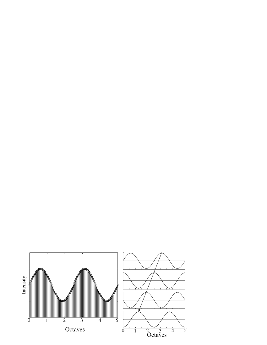
Figure 8: Left: A time slice of the stimulus: 101 tones equally spaced along the logarithmic axis. This ripple has a ripple frequency $\Omega$ of 0.4 cyc/oct with zero phase, and a linear modulation of 50%, against an arbitrary intensity axis (see Equation (4)). Right: the spectral profile changes as a function of time, giving a moving ripple, here with positive frequency (since the phase increases as a function of time).

Five parameters are sufficient to characterize the ripple stimulus:

• The ripple frequency $\Omega$ in cycles/octave,

• The ripple velocity $w$ in Hz, so that a positive value of $w$ and $\Omega$ corresponds to a ripple whose envelope travels towards the low frequencies

• The level or base loudness of the ripple,

• The amplitude of the modulation $\Delta A$ of the ripple around the base,

• The ripple’s initial phase.

Since the tones that make up a ripple are logarithmically spaced, its pitch is indeterminate.

4.2 Data Analysis

In this section, we show the data analysis we apply with the help of a simulation, but to keep the graphs one-dimensional we assume that in Figure 9 and Figure 10, $IR\left(t\right)=\delta\left(t\right)$.

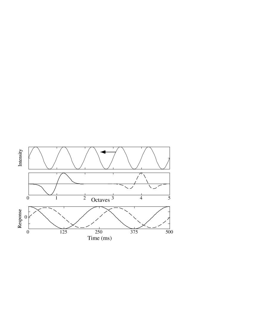
Figure 9: The top panel represents the spectral envelope of the stimulus at a given instant against an arbitrary intensity axis. For the two cells represented in the middle panel (with $IR\left(t\right)=\delta\left(t\right)$), one (unbroken) with the RF centered on low frequencies ($x_{m}=1$, asymmetric with $\phi=90^{o}$), and the other (broken) with the RF centered on high frequencies ($x_{m}=4$, symmetric with $\phi=0^{o}$), the expected responses to a 4 Hz ripple is shown in the bottom panel (unbroken and broken, respectively),against some measure of the response, for instance spikes/sec or the intracellular potential. In our case, the actual response is half-wave rectified, and measured in the form of a spike count, so that the bottom panel should really be seen as a spiking probability that can be measured by measuring the response of the cell to many presentations of the same stimulus.

We use two paradigms to obtain the transfer function of a cell. First, we choose a ripple frequency and present the cell with ripples of varying ripple velocities (typically, -24 Hz to 24 Hz in cortex). Then, for a fixed ripple velocity, we present the cell with ripples of varying ripple frequencies (typically, from -1.6 to 1.6 cyc/oct).

As indicated for a 4 Hz ripple in Figure 9, the response of a cell as a function of time is modulated at the same (temporal) frequency as that of the stimulus. Therefore, we just have to extract the phase and the amplitude of the response. The resulting transfer function for the same two cells is shown in Figure 10. We have presented ripples to the idealized cells shown in panel B. The amplitude of the response as a function of ripple frequency is shown in panel C, whereas the phase of the response is shown in the bottom panel. Note that the phase intercept $\phi$ is $0^{o}$ for the symmetric cells and $90^{o}$ for the antisymmetric cell.

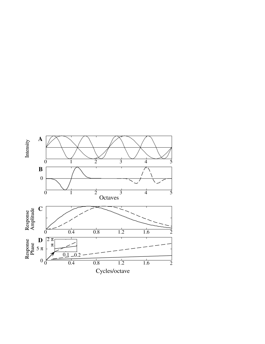
Figure 10: The sounds with the spectrum shown in A (ripples with ripples frequencies of 0 (flat spectrum), 0.4 and 0.8 cycles/octave) are presented at various phases to the two cells in B, as in Figure 9. The amplitude (for instance in spikes/sec) (C) and phase (D) of the best fit to the response are shown.

In the corresponding $\Omega--w$ space, the ripple of Figure 8 corresponds to a pair of points. Therefore, to measure the complete ripple response transfer function of a cell we need to measure its response to all possible ripples, as shown in Figure 11. Note that since cells in cortex respond only to transient stimuli, it is not necessary to present the stimuli along the $w=0$ axis.

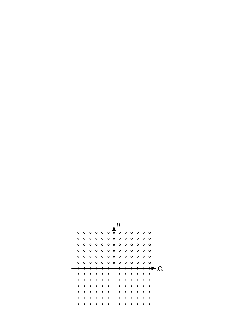
Figure 11: To measure the complete ripple transfer function, we have to measure the response of the cell to all the ripples represented by large circles above. The smallest circles correspond to redundant ripples, as inspection of Eq. (2) and Figure 5 shows.

4.3 Separability

We have shown previously^16,22 that within each quadrant, actual ripple transfer functions are separable : for two fixed values of $\Omega$, the transfer function as a function of $w$ only changes between the two by an overall scale factor and an overall phase. The same is true when $\Omega$ and $w$ are reversed. Hence, one is required only to study two lines in $\Omega-w$ space. Therefore we only need to sample a line in each direction within each quadrant, as shown in Figure 12.

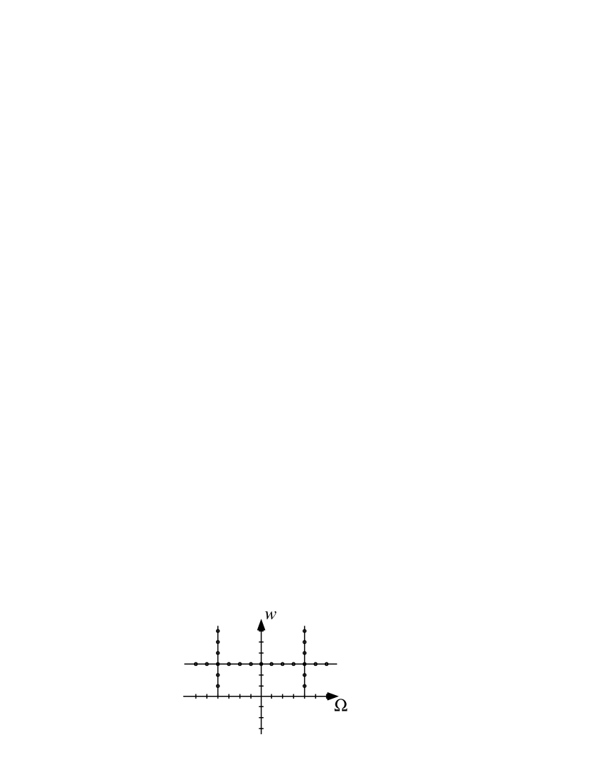
Figure 12: Since we found experimentally that cells have separable transfer functions within each quadrant, it is enough to measure the transfer function along two orthogonal lines in each quadrant.

Without separability, whether full or quadrant, it would be extremely difficult to characterize a cell by its transfer function. Experimentally, given the time required to measure one point of the transfer function, measuring the transfer function at the points indicated in Figure 12 is feasible, whereas measuring the transfer function at all the points indicated in Figure 11 is not.

4.4 Linearity

Linearity is confirmed by comparing the response to combinations of ripples with the response predicted by summing the responses to the individual ripples, i.e. the values of the transfer function. A combination of ripples is computed such that its base loudness is the same as the individual ripples’, and the amplitude of the modulation is scaled as in Equation (4). As an example, to present the combination of two ripples (whose properties are described by subscripts 1 and 2), we compute $B=B_{1}\;\sin\left({2\pi\left({\Omega_{1}\cdot x+w_{1}\cdot t}\right)+\Phi_{1}}\right)+B_{2}\;\sin\left({2\pi\left({\Omega_{2}\cdot x+w_{2}\cdot t}\right)+\Phi_{2}}\right)$. For a modulation of $\Delta A$, the envelope is (in the manner of Equation (4)) $L\,\cdot\left({1+\Delta\kern 1.0ptA\cdot{B\mathord{\left/{\vphantom{B{\max\left(B\right)}}}\right.\kern-1.2pt}{\max\left(B\right)}}}\right)$, where $L$ is the base intensity level. The sound is generated from the envelope using 101 tones over 5 octaves with logarithmically spaced (temporal) frequencies and random (temporal) phases.

5 Experiment and Results

5.1 Experimental Details

Data were collected from domestic ferrets (Mustela putorius). The ferrets were anesthetized with sodium pentobarbital and anesthesia was maintained throughout the experiment by continuous intravenous infusion of either pentobarbital or ketamine and xylazine, with dextrose (in Ringer’s solution) to maintain metabolic stability. The ectosylvian gyrus, which includes the primary auditory cortex, was exposed by craniotomy and the dura reflected. The contralateral ear canal (meatus) was exposed and partly resected, and a cone-shaped speculum containing a miniature speaker was sutured to the meatal stump. For details on the surgery see Shamma et al³.

All stimuli were computer synthesized, gated, and then fed through a common equalizer into the earphone. Calibration of the sound delivery system (to obtain a flat frequency response up to 20 kHz at the level of the eardrum) was performed in situ using a 1/8-in. probe microphone.

Action potentials from single units were recorded using glass-insulated tungsten micro- electrodes with 5-6 M$\Omega$ tip impedances. Neural signals were fed through a window discriminator and the time of spike occurrence relative to stimulus delivery was stored on a computer, which also controlled stimulus delivery, and created raster displays of the responses. In each animal, electrode penetrations were made orthogonal to the cortical surface. In each penetration, cells were typically isolated at depths of 350-600 $\mu$m corresponding to cortical layers III and IV³.

5.2 Obtaining the Transfer Functions

As explained above, we measure the cells’ transfer functions by presenting first, at a fixed ripple frequency, ripples of various velocities. Then, for a fixed ripple velocity, we present ripples of varying ripple frequencies.

5.2.1 Spectral cross-section of the transfer function

A typical example of the analysis is shown in Figure 13. Ripples were presented at 8 Hz, for ripples frequencies from -1.6 cyc/oct to 1.6 cyc/oct in steps of 0.2 cyc/oct, with the ripple starting to move at $t=0ms$, but being acoustically turned on starting at 50 ms with a linear ramping over 8 ms. Each action potential is denoted by a dot on the raster plot in A. One can see the onset response to the ripple at about 70 ms (50 ms + delay due to the ramping up of the stimulus, + latency of the response). Each ripple is presented 15 times. Once the onset activity has died away, the cell goes into a sort of steady-state response. For each ripple frequency, we compute a period histogram starting at 120 ms (this excludes the onset response). Four of those histograms are shown in panel B. To assess the strength and phase of the phase-locked response, we divide the histogram into 16 equal bins. The amplitude and phase of the response is then evaluated by performing a Fourier transform of the data, and extracting the phase of $T\left({\Omega,w=8\ Hz}\right)$ from the first component of the Fourier transform, and the amplitude from

$$T\left({\Omega,w=8\ Hz}\right)=AC_{1}\left(\Omega\right)\cdot{{\left|{AC_{1}\left(\Omega\right)}\right|}\over{\sqrt{\sum\nolimits_{i=1}^{8}{\left|{AC_{i}\left(\Omega\right)}\right|^{2}}}}}$$ (5)

If the modulation of the response were that of a purely linear system, the higher coefficients $AC_{i}(\Omega)$ would be negligible. But because of the half-wave rectification and other non-linearities, they usually are significant. Therefore we weight $AC_{1}(\Omega)$ by the $RMS$ of the other coefficients of the $AC_{i}(\Omega)$ to assess linearity.

The magnitude and phase of the transfer function is shown in panel C. In D, we have inverse Fourier transformed separately the transfer function in quadrant 1 and 2, or equivalently for down- and up-moving ripples, after removing the constant (temporal) phase factor $2\pi w\tau_{d}+\theta$, where $w=8{\rm Hz}$. In this case, the up- and down-moving RFs match very well with each other and with the RF obtained with a two-tone paradigm³.

Note that the period histograms shown in panel B correspond to periods starting at 120 ms, so as to eliminate the effect of the onset response, whereas the second graph in panel C shows phases sent back to 0 ms, at which point in time the phase of the ripples presented were all 0 degrees.

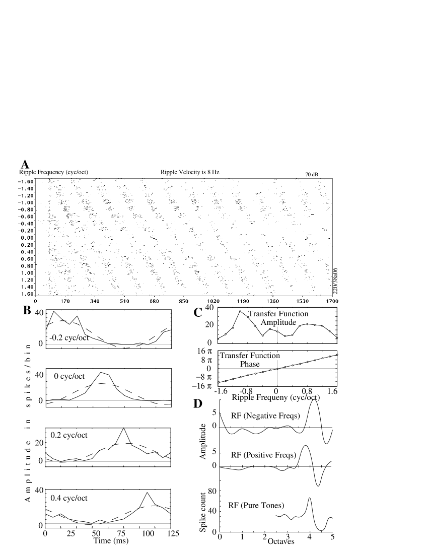
Figure 13: Data analysis using ripples of fixed velocity and varying frequencies. A: Raster plot of responses. Each point represents an action potential, and each paradigm is presented 15 times. B: Period histogram for 4 ripple frequencies. Note how the position of the peak of the best fit changes linearly with ripple frequency. C: Magnitude and phase of the period histogram fits. D: Separate inverse Fourier transforms for positive and negative ripple frequencies of C, obtaining a slice of the RF. Also given for comparison is the response area as determined by the two-tone paradigm. ³

5.2.2 Temporal Cross-Section of the Transfer Function

An example of the extraction of the temporal cross-section of the transfer function for the same cell as in Figure 13 is shown in Figure 14. Ripples are presented at 0.4 cyc/oct, for ripple velocities from -24 Hz to 24 Hz in steps of 4 Hz, with the ripple starting to move at $t=0ms$, being acoustically turned on starting at 50 ms with a linear ramping over 8 ms. Each action potential is denoted by a dot on the raster plot in A. One can see the onset response to the ripple at about 70 ms (50 ms + delay due to the ramping up of the stimulus, + latency of the response). Each ripple is presented 15 times. Once the onset activity dies away, the cell goes into a steady-state response. For each ripple frequency, we compute a period histogram starting at 120 ms (so that the onset response is excluded). Four of those histograms are shown in panel B. To assess the strength and phase of the phase-locked response, we divide the period into 16 equal bins. The amplitude and phase of the response is then evaluated by performing a Fourier transform of the data, and extracting the phase of $T\left({\Omega=0.4\ cyc/oct,w}\right)$ from the first component of the Fourier transform, and the amplitude from

$$T\left({\Omega=0.4\ cyc/oct,w}\right)=AC_{1}\left(w\right)\cdot{{\left|{AC_{1}\left(w\right)}\right|}\over{\sqrt{\sum\nolimits_{i=1}^{8}{\left|{AC_{i}\left(w\right)}\right|^{2}}}}}$$ (6)

If the modulation of the response were that of a purely linear system, the higher coefficients $AC_{i}(w)$ would be negligible. But because of the half-wave rectification and other non-linearities, they usually are significant. Therefore we weight $AC_{1}(w)$ by the RMS of the other coefficients of $AC_{i}(w)$ to assess linearity.

The magnitude and phase of the transfer function is shown in panel C. In D, we have inverse Fourier transformed separately the transfer function in quadrant 1 and 2, or equivalently for down- and up-moving ripples, after removing the constant (spectral) phase factor $2\pi\Omega x_{m}+\phi$, where $\Omega=0.4\ cyc/oct$. In this case, the up- and down-moving IRs match very well with each other.

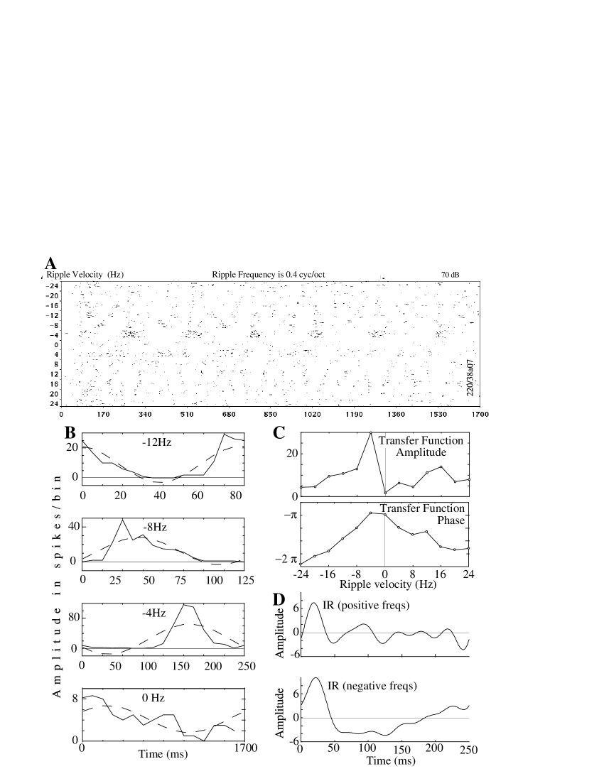
Figure 14: Data analysis using ripples of fixed frequency and varying velocities. A: Raster plot of responses. Each point represents an action potential, and each paradigm is presented 15 times. B: Period histogram for 4 ripple velocities. Note how the peak of the best fit changes linearly with ripple velocity (the 0 Hz case can be used to estimate noise). C: Magnitude and phase of the period histogram fits. D: Separate inverse Fourier transforms for positive and negative ripple velocities of C, obtaining a slice of the IR.

5.3 Quadrant Separability

$RF(x)$ and $IR(t)$, as illustrated in panels D of Figure 13 and Figure 14, are linear combinations of the transfer function evaluated along cross-sections of the $\Omega-w$ plane. Constancy of $RF(x)$ computed for different $w$ is equivalent to proportionality of $T\left({\Omega,w}\right)$ for different $w$ (and similarly for $RF(x)$, $\Omega$, and $T\left({\Omega,w}\right)$). This was the requirement given above to verify quadrant separability. This has all been verified for many cells in the first quadrant¹⁶. While it is theoretically possible for the remaining independent quadrant to be nonseparable, it seems unlikely in ferrets, humans, and most mammals (possible exceptions might include sonar-using animals, which could require further specialization). We are currently verifying separability in the second quadrant.

Shown in Figure 15 are examples of the positive-frequency RF and positive-frequency IR for two cells, as computed at the different sections indicated.

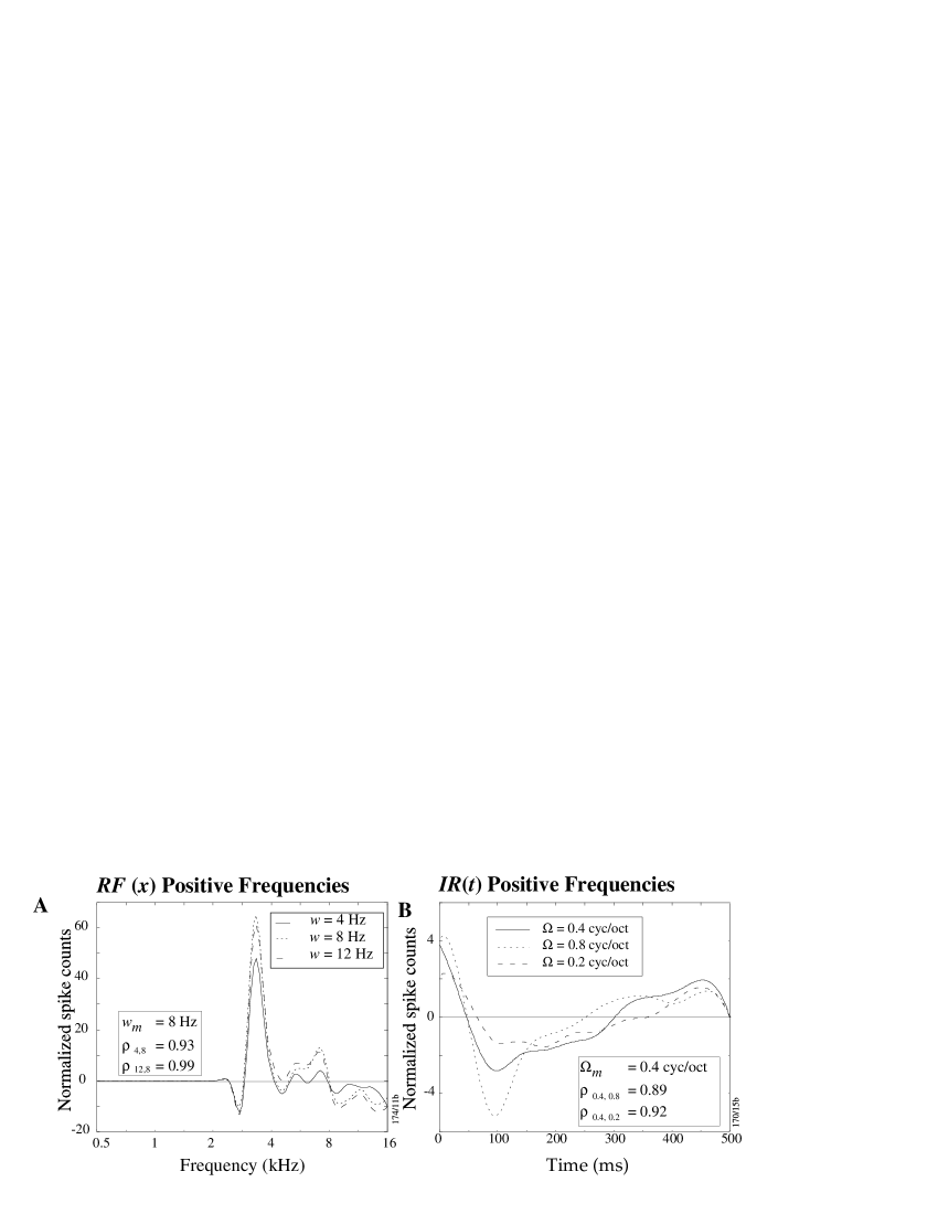
Figure 15: Left The positive-frequency RF computed at constant ripple velocity for 3 different ripple velocities. The shapes should be the same if the system is separable. Right The positive-frequency IR at constant ripple frequency for 3 different ripple frequencies. The shapes should be the same if the system is separable.

5.4 Quadrant Linearity

Linearity has been verified by presenting cells with a combination of ripples from different quadrants^16,22,23. As shown in Figure 16 for one cell, the correlation between the predicted and the measured response is (as in most cases) very good. Note that the predicted response is shown in its non-half-wave rectified version: as cells do not have negative firing rates, and the pentobarbital anesthetic has reduced the spontaneous activity to zero, the comparison should be made between the actual response and the half-wave rectified version of the predicted response. The correlation coefficient $\rho$ in Figure 16 is the cross-correlation between the measured and the predicted response. We have previously presented the correlation between prediction and response within a single quadrant for 55 cells and found 84% of the cells with $\rho>0.6$.²² The error bars on the measured response show the variability of cortical cells’ responses from sweep to sweep. Disparity is maximal between the prediction and the actual spike count where both are small.

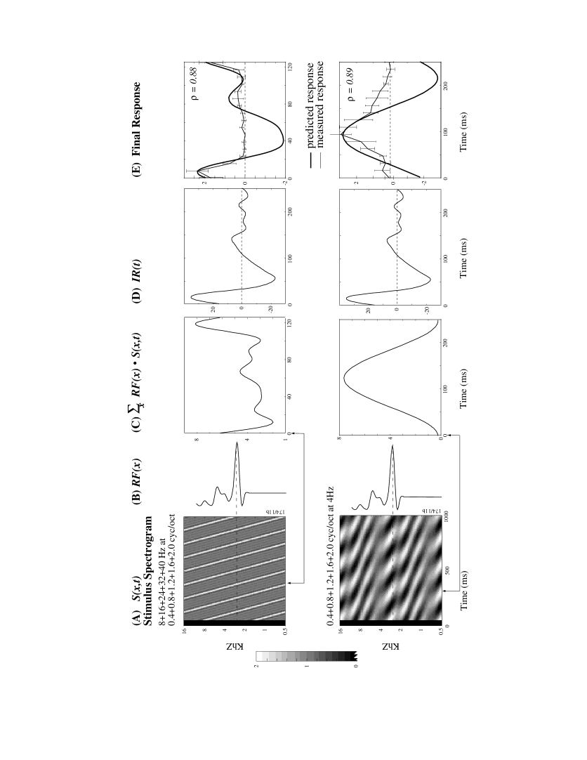
Figure 16: Linearity and separability within one quadrant. The stimulus (spectrogram in A) is presented to a cell (RF shown in B). To predict the response, we multiply the spectrogram with the RF (C), convolve the result with the IR in D, obtaining the predicted response in E, the half-wave rectified version of which should be compared with the actual response. Spontaneous activity is zero in this anesthetized preparation, and that the ordinate axis is in arbitrary coordinates, except for the measured response in E which is in spikes/sec.

5.5 Full-Quadrant Separability and Linearity

The remainder of this discussion describes logical extensions that are currently under study. Thus far we have only verified separability in a single quadrant. In vision, some cortical simple cells are fully separable²⁴, but all are at least quadrant separable²⁵. We have found both types in the auditory cortex as well; Figure 17 shows examples of each. A fully separable cell has an STRF that is a simple product of an RF and an IR, as in A. A quadrant separable cell, as in B, does not, since it has different responses for upward and downward moving ripples (as can be seen by inspection of its $STRF(x,t)$: it is not symmetric about $x_{m}$). The separability of a cell does not affect the linearity of responses to ripple combinations.

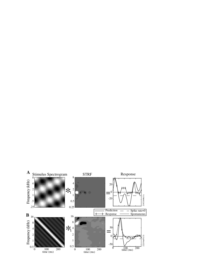
Figure 17: Predictions of responses to complex dynamic spectra using the STRF. A The predicted response is computed by a convolution (along the time dimension) of the STRF with the spectrogram. The stimulus shown is composed of two ripples (0.4 cycles/octave at 12 Hz and -4 Hz). The predicted waveform is shown juxtaposed to the actual response (crosses) over one period of the stimulus, in spikes/bin summed over 30 sweeps. B Another example: the stimulus consists of a combination of ripples with ripple frequencies 0.2 cycles/octave at 4 Hz, 0.4 cycles/octave at 8 Hz, … 1.2 cycles/octave at 24 Hz, in cosine phase, resulting in an FM-like stimulus. In this Ketamine/Xylazine preparation, the spontaneous activity was non-zero.

5.6 Response Characteristics

The transfer function for a specific cell is typically tuned to a characteristic ripple frequency and velocity. The population of cells shows a wide range of characteristic ripple frequencies and velocities. Characteristic ripple velocities are mostly in the 8 - 16 Hz range, rarely exceeding 30 Hz, and characteristic ripple frequencies are mostly in the 0.4 - 0.8 cycles per octave range, rarely exceeding 2 cycles per octave (in this anesthetized preparation). The slope of the transfer function as a function of ripple frequency, $x_{m}$, corresponds to the center frequency of the spectral envelope, which ranges from 200 Hz to at least 24 kHz (above which our acoustic delivery system is inadequate). The slope of the transfer function as a function of ripple velocity, $\tau_{d}$, corresponds to the center of the temporal envelope, which ranges roughly from 10 ms to 60 ms. The RF symmetry $\phi$, which describes the effects of lateral inhibition and excitation, ranges roughly from $-90^{o}$ to $+90^{o}$ (out of a possible $-180^{o}$ to $+180^{o}$), clustered around $0^{o}$. The IR polarity $\theta$, which describes the polarity of the temporal response, ranges roughly from $45^{o}$ to $135^{o}$ (out of a possible $0^{o}$ to $180^{o}$).

6 Conclusions

The emphasis in this review has been on presenting a technique to describe neural response patterns of units in the cortex. More precisely, we use moving ripples to characterize the response fields of auditory cortical neurons, although this is a general method that can be used anywhere responses are shown to be substantially linear for broadband stimuli.

Practically, we find that because of linearity of cortical responses with respect to spectral envelope, we can use the ripple method to characterize auditory cortical cell responses to dynamic, broadband sounds. The linearity of the cortical unit responses is quantified by the correlation coefficient between the predicted and the measured responses curves. While at this point we do not have statistics to quantify the linearity of response to ripples moving in both directions, linearity within one quadrant (to down-moving ripples) has been extensively quantified²², and we have no reason to expect linearity be any different for ripples moving in both directions. The separability of cells makes the ripple method practical, because of the time needed to characterize a cell. One advantage of the method is the simultaneous probing of spectral and temporal characteristics. Temporal processing is becoming more and more recognized as an essential part of cortical function, and the ripple method places it on an equal footing with spectral processing. A caveat is that, thus far, the method only has been applied to the steady state (i.e. periodic) response of cells.

We find that response fields in AI tend to have characteristic shapes both spectrally and temporally. Specifically, AI cells are tuned to moving ripples, i.e., a cell responds well only to a small set of moving ripples around a particular spectral peak spacing and velocity. We find cortical cells with all center frequencies, all spectral symmetries, bandwidths, latencies and temporal impulse response symmetries. One way to interpret this result is that AI decomposes the input spectrum into different spectrally and temporally tuned channels. Another equivalent view is that a population of such cells, tuned around different moving ripple parameters, can effectively represent the input spectrum at multiple scales. For example, spectrally narrow cells will represent the fine features of the spectral profile, whereas broadly tuned cells represent the coarse outlines of the spectrum. Similarly, dynamically sluggish cells will respond to the slow changes in the spectrum, whereas fast cells respond to rapid onsets and transitions. In this manner, AI is able to encode multiple different views of the same dynamic spectrum. From this, we conclude that the primary auditory cortex performs multi-dimensional, multi-scale wavelet transform of the auditory spectrum.

Pitch is very important to the auditory system. The spectral ripple responses presented here do not have pitch, since they are synthetized with logarithmically spaced carrier tones. We have not yet examined unit responses to a ripple spectra with harmonically related carrier tones. Consequently, all our unit responses are due to the envelope or spectral profile of the broadband stimulus, and are not dependent on the carrier tones. It is quite possible that the pitch of a harmonic series of tones will affect the responses. It is also possible that sufficiently narrowly tuned cells might directly encode the harmonic spacing in a spectrum in a systematic manner to encode the pitch as was discussed in detail in Wang and Shamma²⁶. This is work in progress.

The suggestion that cortical cells are linear might appear far-fetched given the non-linear response to pure tones, such as rate vs. intensity functions with threshold, saturation, and non- monotonic behavior (Brugge and Merzenich²⁷; Nelken et al.⁸). Nevertheless, we find that the non-linearity observed with broadband ripple spectra is substantially smaller than with tonal stimuli, when it comes to predicting the response of a cell to a combination of stimuli, knowing the response to individual ones. Furthermore, just as measuring linear systems response properties with tones, such as bandwidth, rate-level functions, tuning quality factor and other measures is considered meaningful, characteristics of the ripple responses prove useful, and relate to the properties measured with tones^18,16. Investigations currently under way in the Inferior Colliculus will shed light on the mechanisms that allow cells to exhibit a linear behavior in auditory cortex, so many synapses away from the auditory nerve.

7 Acknowledgements

This work is supported by a MURI grant N00014-97-1-0501 from the Office of Naval Research, a training grant NIDCD T32 DC00046-01 from the National Institute on Deafness and Other Communication Disorders, and a grant NSFD CD8803012 from the National Science Foundation. We would like to thank David Klein, Izumi Ohzawa and Alan Saul.

8 References

1. M.M. Merzenich, P.L. Knight and G.L. Roth, Representation of the cochlear partition on the superior temporal plane of the macaque monkey, Brain Res. 50, 231-249 (1975). R.A. Reale and T.J. Imig, Tonotopic organization in auditory cortex of the cat, J. Comp. Neurol. 192, 265-291 (1980).

2. J.C. Middlebrooks, R.W. Dykes and M.M. Merzenich, Binaural response-specific bands in primary auditory cortex of the cat: topographical organization orthogonal to isofrequency contours, Brain Res. 181, 31-48 (1980).

3. S.A. Shamma, J.W. Fleshman, P.R. Wiser and H. Versnel, Organization of response areas in ferret primary auditory cortex, J. Neurophys. 69, 367-383 (1993).

4. C.E. Schreiner, J. Mendelson and M.L. Sutter, Functional topography of cat primary auditory cortex: representation of tone intensity, Exp. Brain Res. 92, 105-122 (1992).

5. C.E. Schreiner and M.L. Sutter, Topography of excitatory bandwidth in cat primary auditory cortex: single- versus multiple-neuron recordings, J. Neurophysiol. 68, 1487-1502 (1992).

6. J. Mendelson, C.E. Schreiner, M.L. Sutter and K. Grasse, Functional topography of cat primary auditory cortex: selectivity to frequency sweeps, Exp. Brain Res. 94, 65-87 (1993).

7. R.L. De Valois and K.K. De Valois, Spatial Vision, Oxford University Press, New-York (1988).

8. I. Nelken, Y. Prut, E. Vaadia and M. Abeles, Population responses to multifrequency sounds in the cat auditory cortex: One- and two-parameter families of sounds, Hear. Res. 72, 206-222 (1994).

9. M.L. Sutter,.W.C. Loftus and K.N. O’Connor, Temporal properties of two-tone inhibition in cat primary auditory cortex, ARO midwinter meeting (1996).

10. L.R. Rabiner and R.W. Schafer, Digital processing of speech signals, Prentice-Hall, New-Jersey (1978).

11. J.E. Rose, J.F. Brugge, D.J. Anderson and J.E. Hind, Phase-locked response to low-frequency tones in single auditory nerve fibers of the squirrel monkey, J. Neurophys. 30, 769-793 (1967).

12. W.S. Rhode and P.H. Smith, Encoding time and intensity in the central cochlear nucleus of the cat, J. Neurophys. 56, 262-286 (1986).

13. W.S. Rhode and S. Greenberg, Physiology of the cochlear nuclei, in The mammalian auditory pathway: Neurophysiology, Popper, A.N. and Fay, R.R. editors, Springer-Verlag, New-York (1991).

14. R. Lyon and S.A. Shamma, Timbre and pitch, in Auditory computation, H.L. Hawkins., T.A. McMullen, A.N. Popper and R.R. Fay, editors, Springer-Verlag, New-York (1995).

15. G. Langner, Periodicity coding in the auditory system, Hearing Res. 6, 115-142 (1992). D.A. Depireux, D.J. Klein, J.Z. Simon and S.A. Shamma, Neuronal correlates of pitch in the Inferior Colliculus, ARO midwinter meeting (1997).

16. N. Kowalski, D.A. Depireux and S.A. Shamma, Analysis of dynamic spectra in ferret primary auditory cortex: I. Characteristics of single unit responses to moving ripple spectra, J. Neurophys. 76, (5) 3503-3523 (1996).

17. D.K. Ryugo, The auditory nerve: peripheral innervation, cell body morphology, and central projections, in The mammalian auditory pathway: neuroanatomy, D.B. Webster, A.N. Popper, and R.R. Fay, editors, Springer-Verlag, New-York, (1991).

18. C.E. Schreiner and B.M. Calhoun, Spatial frequency filters in cat auditory cortex. Auditory Neurosci. 1, 39-61 (1994). S.A. Shamma, H. Versnel and N. Kowalski, Ripple analysis in ferret primary auditory cortex: I. Response characteristics of single units to sinusoidally rippled spectra. Auditory Neurosci. 1, 233-254 (1995). S.A. Shamma and H. Versnel, Ripple analysis in ferret primary auditory cortex: II. Prediction of unit responses to arbitrary spectral profiles. Auditory Neurosci. 1, 255-270 (1995). H. Versnel, N. Kowalski and S.A. Shamma, Ripple analysis in ferret primary auditory cortex: III. Topographic distribution of ripple response parameters. Auditory Neurosci. 1, 271-285 (1995).

19. A. Papoulis, The Fourier integral and its applications, McGraw-Hill (1962).

20. L. Cohen, Time-frequency analysis, Prentice-Hall, New Jersey (1995).

21. D. Dong and J.J. Atick, Temporal decorrelation: a theory of lagged and nonlagged cells in the lateral geniculate nucleus, Network: Computation in Neural Systems 6, 159-178 (1995).

22. N. Kowalski, D.A. Depireux and S.A. Shamma, Analysis of dynamic spectra in ferret primary auditory cortex: II. Prediction of unit responses to arbitrary dynamic spectra. J. Neurophys. 76, (5) 3524–3534 (1996).

23. J.Z. Simon, D.A. Depireux and S.A. Shamma, Representation of complex dynamic spectra in auditory cortex, in Psychophysical and physiological advances in hearing, A.R. Palmer, A.Rees, A.Q. Summerfield and R. Meddis, editors, Whurr Publishers, London (1988).

24. J. McLean and L.A. Palmer, Organization of simple cell responses in the three-dimensional frequency domain. Vis. Neurosc. 11, 295-306 (1994). G.C. DeAngelis, I. Ohzawa and R.D. Freeman, Receptive-field dynamics in the central visual pathways. Trends Neurosc. 18, 451-458 (1995).

25. B.W. Andrews and D.A. Pollen, Relationship between spatial frequency selectivity and receptive field profile of simple cells, J. Physiol. (London) 287, 163-176 (1979). S.M. Friend and C.L. Baker, Spatio-temporal frequency separability in area 18 neurons of the cat, Vision Res. 33, 1765-1771 (1993).

26. K. Wang and S. A. Shamma, Self-normalization and noise robustness in auditory representations. IEEE Trans. Audio. Speech. Proc. 2, 421-435 (1994).

27. J. F. Brugge and M. M. Merzenich, Responses of neurons in auditory cortex of the Macaque monkey to monaural and binaural stimulation. J. Neurophysiol. 36, 1138-1158 (1973).