Abstract

We analyze the control of frequency for a synchronized inhibitory neuronal network. The analysis is done for a reduced membrane model with a biophysically-based synaptic influence. We argue that such a reduced model can quantitatively capture the frequency behavior of a larger class of neuronal models. We show that in different parameter regimes, the network frequency depends in different ways on the intrinsic and synaptic time constants. Only in one portion of the parameter space, called ‘phasic’, is the network period proportional to the synaptic decay time. These results are discussed in connection with previous work of the authors, which showed that for mildly heterogeneous networks, the synchrony breaks down, but coherence is preserved much more for systems in the phasic regime than in the other regimes. These results imply that for mildly heterogeneous networks, the existence of a coherent rhythm implies a linear dependence of the network period on synaptic decay time, and a much weaker dependence on the drive to the cells. We give experimental evidence for this conclusion.

Key words: gamma oscillations, hippocampus, interneurons, synchronization

Section 1 Introduction

Coherent neuronal oscillations have been implicated widely as a correlate of brain function [Gray (1994), Llinás and Ribary (1993)]. However, our understanding of the mechanisms underlying such activity is still in its infancy. (See ? (?) and ? (?) for recent reviews). It has been demonstrated experimentally [Whittington et al. (1995), Jefferys et al. (1996)], computationally [Wang and Rinzel (1992), Whittington et al. (1995)], and analytically [van Vreeswijk et al. (1994), Gerstner et al. (1996), Terman et al. (1997)] that mutual inhibition can generate stable synchronous oscillations. Previous analytical work mostly concentrated on the mechanisms responsible for synchronization. Here we address the mechanisms for controlling the network frequency and the interplay between frequency and synchronization.

Previously [White et al. (1998)], we showed that synchronization of inhibitory networks can occur in a wide range of frequencies for homogeneous neurons, but in the presence of heterogeneity network synchronization is very fragile in some parameter regimes. We have identified a pair of parameter regimes, denoted ‘phasic’ and ‘tonic’; in the former some coherence is maintained in the presence of mild heterogeneity, while in the latter it is lost. In this paper, we relate these regimes to the parameters that determine the frequency of the network when it is synchronized.

There are three important time constants in the network dynamics. One is an intrinsic time constant of the uncoupled cell, dependent on the conductances and the capacitance of the membrane. The second is the decay time of the inhibition. The third, the network period, depends on the other two time scales and other parameters, notably the synaptic conductance and injected current. The aim of this paper is to understand how the first and second time constants influence the third.

We show that there are three asymptotic regimes, in which the network period varies differently as the inhibitory time constant is changed. Two of these are the tonic and phasic [White et al. (1998)] regimes mentioned above and the third we call ‘fast’. In the tonic regime, the period is small compared with both the intrinsic time scale and the synaptic decay time. In this regime, we show that the network frequency is only weakly dependent on the inhibitory decay time; indeed, the frequency is affected mainly by the average amount of inhibition, not by the time course of that inhibition. In the phasic regime, the intrinsic membrane time scale is small compared with the network period and the synaptic decay time. In this regime, we show that the network period is proportional to the decay time, with the proportionality constant a function of other network parameters. In the fast regime, the synaptic decay time is short compared to the network period. In this regime, the period is dominated by the intrinsic time constant. We give constraints on the network parameters (intrinsic membrane time scale, synaptic decay time, synaptic conductance and applied current) for the network to fall into each of the three asymptotic regimes.

The three regimes can be related to the behavior of the network in the presence of mild heterogeneity , as shown numerically in White et al. (?). In the fast regime, the synaptic influence acts as a brief inhibitory pulse which has been shown to lead to stable anti-synchronous oscillations [Friesen (1994), Perkel and Mulloney (1974), Skinner et al. (1994), van Vreeswijk et al. (1994), Wang and Rinzel (1992)]. In the phasic and tonic regimes, synchrony through inhibition is fairly robust for homogeneous networks of neurons over a wide range of network frequencies [van Vreeswijk et al. (1994), Gerstner et al. (1996)]. However, it is very fragile when even mild heterogeneity is included [Golomb and Rinzel (1993), Wang and Buzsáki (1996), White et al. (1998)]. We showed that the loss of coherence of the network happens by different mechanisms in the tonic and phasic regimes [White et al. (1998)]. In the tonic regime, mildly heterogeneous networks are effectively de-coupled and exhibit asynchrony (loss of phase relationships among the cells); in the phasic regime, the network can lose some coherence via suppression, in which the slower cells receive enough inhibition to prevent their firing.

Our analytical work uses a reduced membrane description for the neuron with a biophysically-based synaptic model. The analysis is for a homogeneous network; when considering the frequency of a synchronous solution, we can regard the network as a single self-inhibited neuron. We show that in the phasic regime, the synaptic current dominates and the actual intrinsic membrane dynamics are not as important for the firing frequency. In the tonic regime, the intrinsic dynamics do become more important. We give a comparison between our analytical estimates for the period and those obtained numerically for conductance-based neuron models.

The work in this paper, in conjunction with ? (?) shows that, in the presence of mild heterogeneity, the control of frequency is strongly tied to the time scale of the mechanism that produces the synchronization. That is, in order to have coherence for a mildly heterogeneous system, the latter must be in the phasic regime, which then implies that the frequency is controlled by the time constant of the inhibitory decay. It was found experimentally and numerically that the frequency of coherently firing interneurons in the CA1 region of the hippocampus is strongly dependent on the decay time of the inhibitory synapse [Whittington et al. (1995), Jefferys et al. (1996), Traub et al. (1996a), Wang and Buzsáki (1996)]. The analytical work given in this paper clarifies the reasons for this frequency behavior as well as the remark found in many papers that the inhibitory decay time can be a critical factor in the determination of the network frequency [Destexhe et al. (1993), Skinner et al. (1993), Kopell and LeMasson (1994)].

Section 2 Neuron model

We consider the frequency control of so called Type I neuronal dynamics [Hansel et al. (1995), Ermentrout (1996)] and examine simplifications that would make it more amenable to analysis. These neurons are distinguished by the fact that they have positive phase response curves (PRC) [Hansel et al. (1995)]. i.e. a positive depolarizing current always advances the time of the next spike. It has been shown recently that neurons which admit very low frequency oscillations near the critical applied current are Type I [Ermentrout (1996)] although the converse is not necessarily true. We note that the type of bifurcation to firing of the neuron is not important for our analysis. Type I neurons have been used to represent inhibitory interneurons in the hippocampus [Traub et al. (1996a), Wang and Buzsáki (1996), White et al. (1998)].

We consider an inhibitory network of single-compartment neurons with membrane potential dynamics of the form [Rinzel and Ermentrout (1989), Ermentrout (1996), Hansel et al. (1995), Wang and Buzsáki (1996), White et al. (1998)]

$$C\frac{dV_{i}}{d\tilde{t}}=\tilde{I}_{i}-\sum I_{\rm ion}-I_{s},$$ (1)

where $\tilde{I}_{i}$ is an applied current, $I_{\rm ion}$ are the ionic currents responsible for spike generation and recovery and $I_{s}$ is the synaptic current induced by the spikes of other neurons coupled pre-synaptically. The ionic currents $I_{\rm ion}$ are functions of potential and the dependent dynamical variables, which are in turn governed by a system of differential equations. In the Appendix we give the equations for two conductance-based neuron models [White et al. (1998), Ermentrout and Kopell (1998)], which are Type I or at least very close to Type I (data not shown). Figure 1 shows example voltage traces for the two models. The coupling between the neurons is exclusively through chemical synapses represented by the synaptic current which takes the form $I_{s}=\tilde{g}S(\tilde{t})(V-V_{s})$, where

$$\frac{dS}{d\tilde{t}}=\tilde{\alpha}F(V_{pre})(1-S)-\tilde{\beta}S,$$ (2)

$\tilde{\alpha}$ and $\tilde{\beta}$ are respectively the synaptic rise and decay rates, $V_{pre}$ is the membrane potential of the pre-synaptic neuron, and $F(V)=1/(1+\exp[-V])$. We will often consider the synaptic decay time $\tilde{\tau}\equiv\tilde{\beta}^{-1}$.

We approximate the full conductance-based dynamics with integrate-and-fire dynamics where the firing of the neuron is represented by the resetting of the membrane potential whenever it crosses a threshold. Our justification for using this approximation hinges on three considerations: 1) both the conductance-based and integrate-and-fire models are Type I (in the sense of positive PRC), 2) the action potentials (spike widths) are narrow compared to their typical spiking period so the frequency is dominated by the membrane recovery time, and 3) the time scale for spike generation is very fast compared to the recovery time so an effective threshold for spiking can be defined. The first point was verified by observing that the measured PRC of the conductance-based models near the bifurcation to firing is positive.

We model the approach to threshold with a simple passive decay to obtain dynamics governed by a single equation of the form:

$$C\frac{dV}{d\tilde{t}}\simeq\tilde{I}-g_{m}(V-V_{r})-\tilde{g}S(\tilde{t})(V-V_{s}),$$ (3)

where $g_{m}$ is an effective membrane recovery conductance, $V_{r}$ is an effective membrane reversal potential and $V_{s}$ is a synaptic reversal potential. $V(t)$ is reset to $V_{0}$ whenever it reaches the threshold potential $V_{T}$. The passive decay to threshold is a very good approximation for some neuronal models such as the reduced Traub and Miles model given in the Appendix [Ermentrout and Kopell (1998)]. On the other hand, we will show that even when the passive decay is not a good approximation to the slow dynamics of the neuron model, it can still adequately describe the frequency behavior, especially in the phasic regime where the synaptic current dominates.

The synaptic current $S(\tilde{t})$ is generated from the spikes of pre-synaptic neurons. This must be emulated in the reduced model (3). Here we consider $S(\tilde{t})$ to be an arbitrary time dependent function. In Sec. 3, we analyze some biophysical synaptic models in detail and explicitly derive the time course of $S(\tilde{t})$ in response to a pre-synaptic spike.

To simplify the analysis, we rescale Eq. (3) so that only dimensionless parameters remain. The voltage can be rescaled via $v=(V-V_{0})/(V_{T}-V_{0})$, so that the reset potential is at $v=0$ and the threshold is at $v=1$. We define an intrinsic membrane decay time

$$\tau_{m}\equiv C/g_{m}$$ (4)

and rescale time by $t=\tilde{t}/\tau_{m}$. This scaling takes the membrane time scale to 1, leading to the dimensionless equation

$$\frac{dv}{dt}=I-[1+\gamma S(t)]v-gS(t),$$ (5)

where

$$I=\frac{\tilde{I}+I_{r}}{I_{T}},\qquad g=\frac{\tilde{g}}{g_{T}},\qquad\gamma=\frac{\tilde{g}}{g_{m}},$$ (6)

with $I_{T}=g_{m}(V_{T}-V_{0})$, $I_{r}=g_{m}(V_{r}-V_{0})$, and $g_{T}=I_{T}/(V_{0}-V_{s})$. The neuron is said to fire each time $v(t)$ reaches 1, whereupon it immediately resets to $v=0$. It is important to note that this does not restrict $v(t)$ to nonnegative values away from $t=0$.

An even simpler model is

$$\frac{dv}{dt}=I-v-gS(t).$$ (7)

which follows from Eq. (5) if $\gamma<<1$. We refer to the reduced model given by Eq. (5) as model 1 and the one given by Eq. (7) as model 2. The two models differ in that the synapse acts solely as a forcing function in model 2, but also affects the membrane decay rate in model 1. As we will show, the frequency behavior of the two models is qualitatively similar even if $\gamma$ is not small. We will focus most attention on model 2 in our analysis. The synchronization tendencies of model 2 for slow synapses has been studied thoroughly [van Vreeswijk et al. (1994), Hansel et al. (1995), Gerstner et al. (1996), Chow (1998)].

Section 3 Synaptic Model

In conductance-based neuron models, the post-synaptic current is initiated by a pre-synaptic spike. In the reduced model, the spikes have been eliminated so this process must be modeled. We do so by deriving the synaptic time course for Eq. (2) explicitly for a stereotypical pre-synaptic spike. As we will show below, the spike response can be described by a time dependent recursive forcing function of the form

$$S(t)\rightarrow a(t-t_{l})S(t)+S_{f}(t-t_{l}),$$ (8)

where $S(t)$ is the synaptic gating variable to be used in Eq. (5), $t_{l}$ gives the spiking times of the pre-synaptic neuron, $S_{f}(t)$ is the stereotypical post-synaptic response, and $a(t)$ is a ‘memory’ function. (Note that all time and rate parameters have been rescaled by $\tau_{m}$ in this section). We divide synapses into two types – saturating and nonsaturating. If the synaptic variable $S(t)$ increases without bound as the rate of firing of the pre-synaptic cell approaches infinity then we call this a nonsaturating synapse. If however, $S(t)$ saturates to a fixed value as the firing rate approaches infinity then we call this a saturating synapse. The behavior of the function $a(t)$ determines the type of the synapse.

We first derive the recursion relation explicitly for a simple nonsaturating synaptic model given by

$$\frac{dS}{dt}=-S/\tau+\sum_{l=0}^{N}\delta(t-t_{l}),$$ (9)

where $t_{l}$ denotes the times of the pre-synaptic spikes. Synapses of this form have been considered in previous models [Abbott and van Vreeswijk (1993), Tsodyks et al. (1993), van Vreeswijk et al. (1994), Hansel et al. (1995)]. Integrating Eq. (9) results in

$$S(t)=S(0)e^{-t/\tau}+\sum_{l=0}^{N}e^{-(t-t_{l})/\tau},$$ (10)

where we begin the integration at $t=0$. This sum is equivalent to the recursion relation

$$S(t)\rightarrow S(t)+e^{-(t-t_{l})/\tau}.$$ (11)

Here $a(t)=1$ and $S(t)$ increases without bound as the frequency increases.

Now consider the synaptic model in the Appendix. We will show that this is a saturating synapse. When the pre-synaptic neuron fires, $F(V_{\rm pre})$ in Eq. (2) rises from near zero to a value near unity, then returns to zero. The precise shape is determined by the temporal characteristics of the action potential and $F(V)$. Our analysis is similar to that of ? (?). We assume that the shape of $F(V)$ can be approximated by a square pulse with a width of $\Delta t$, given by the time the membrane potential remains above zero during an action potential (i.e. width of the spike). We consider a train of square pulses arriving at times $t_{l}$, with $t_{l}+\Delta t<t_{l+1}$  $\forall\,l$ (i.e. no overlapping spikes). The synaptic response is then found from

$$\frac{dS}{dt}=\alpha Q(t)(1-S)-\beta S,$$ (12)

$$Q(t)=\sum_{l=-\infty}^{\infty}H(t-t_{l}),$$ (13)

where $H(t)$ is a square pulse of unit height with rise at $t=0$ and fall at $t=\Delta t$.

Given $l$, we define

$$R(t)\equiv\alpha\int_{t_{l}}^{t}Q(t^{\prime})dt^{\prime}=\left\{\begin{array}[]{ll}\alpha(t-t_{l}),&t_{l}\leq t\leq t_{l}+\Delta t\\ \alpha\Delta t,&t_{l}+\Delta t<t<t_{l+1}\end{array}\right.$$ (14)

and then integrate (12) from $t_{l}$ to $t<t_{l+1}$ to yield

$$S(t) = e^{-R(t)-\beta t}\left[S(t_{l})e^{\beta t_{l}}+\int_{t_{l}}^{t}\alpha Q(t^{\prime})e^{R(t^{\prime})+\beta t^{\prime}}dt^{\prime}\right]$$ (15)

$$= \left\{\begin{array}[]{ll}e^{-\alpha(t-t_{l})}(S(t_{l})e^{-\beta(t-t_{l})})+\left(\frac{\alpha}{\alpha+\beta}\right)\left(1-e^{-(\alpha+\beta)(t-t_{l})}\right),&t_{l}\leq t\leq t_{l}+\Delta t\\ e^{-\alpha\Delta t}(S(t_{l})e^{-\beta(t-t_{l})})+\left(\frac{\alpha}{\alpha+\beta}\right)\left(1-e^{-(\alpha+\beta)\Delta t}\right)e^{-\beta(t-t_{l}-\Delta t)},&t_{l}+\Delta t<t<t_{l+1}\end{array}\right.$$ (18)

Consider $S(t)$ at the time of the next spike, $t=t_{l+1}$. If the spike does not occur, $S(t)$ will continue to decay exponentially with rate $\beta$, i.e.

$$\begin{array}[]{ll}S(t)=S(t_{l+1})\exp(-\beta(t-t_{l+1})),&t_{l+1}<t.\end{array}$$ (19)

We can thus rewrite Eq. (18) as a recursion relationship with the spike at $t_{l+1}$ as

$$S(t)\rightarrow a(t-t_{l+1})S(t)+S_{f}(t-t_{l+1})$$ (20)

where

$$a(t)=\left\{\begin{array}[]{ll}e^{-\alpha t},&0\leq t\leq\Delta t,\\ e^{-\alpha\Delta t},&\Delta t<t,\end{array}\right.$$ (21)

and

$$S_{f}(t)=\left\{\begin{array}[]{ll}(\frac{\alpha}{\alpha+\beta})(1-e^{-(\alpha+\beta)t}),&0\leq t\leq\Delta t,\\ (\frac{\alpha}{\alpha+\beta})\left(1-e^{-(\alpha+\beta)\Delta t}\right)e^{-\beta(t-\Delta t)},&\Delta t<t.\end{array}\right.$$ (22)

The $S(t)$ appearing in the right hand side of Eq. (20) is understood to be the function that would occur in the absence of a new spike, Eq. (19).

In contrast to Eq. (11), there is a multiplicative factor $a(t)$ which ‘damps’ away the past. For $a(t)<1$, $S(t)$ always saturates to a finite value. $S_{f}(t)$ and $a(t)$ have discontinuous first derivatives because a square pulse was used as input, but in general the functions will be smooth.

Depending on the values of the three parameters $\alpha$, $\beta$ and $\Delta t$, the synaptic time course can take on many shapes. Here we are concerned with narrow spikes (small $\Delta t$) and slowly decaying inhibition ($\beta<<\alpha$). If the rise time is very fast, we can explicitly take the double limit $\alpha\rightarrow\infty$, $\Delta t\rightarrow 0$, $\alpha\Delta t=c$, where c is a constant, to get

$$S_{f}(t)=(1-e^{-c})e^{-\beta t}.$$ (23)

and $a=e^{-c}$.

The constant $c$ is the ratio of the spike width to the rise time of the synaptic current, and determines the contribution from the past to the current synaptic response. If $c$ is large enough we can reasonably ignore the past and use the approximation $a\simeq 0$ and $S_{f}(t)\simeq\exp(-\beta t)$. Then the synaptic update function to be used in Eqs. (5) and (7) takes the form

$$S(\tilde{t})\rightarrow e^{-(t-t_{l})/\tau},$$ (24)

where $\tau=\tilde{\tau}/\tau_{m}$ is the rescaled synaptic decay time. Equation (24) gives the recursion relation for the synapse where $a(t)=0$ and is valid in the limit where the rise time of the synaptic gating variable is very fast compared to the spike width. We note that a nonzero rise time is very important for synchronization [van Vreeswijk et al. (1994), Hansel et al. (1995), Gerstner et al. (1996), Terman et al. (1997), Chow (1998)] but it is not as important for frequency determination.

Section 4 Period of a synchronized network

In this section we will derive the form of the network period analytically for model 2 [Eq. (7)] in terms of a transcendental relation for saturating and non-saturating synapses. We will also analyze the differences that would result if we considered model 1 [Eq. (5)]. In general the same qualitative behavior holds between the two reduced models. To calculate the period for the reduced models, we assume the neuron spikes repeatedly with a period $T$ (the frequency is defined as $f=T^{-1}$). We then integrate the membrane equation from the time of the last spike to the time of the next spike. The period is obtained self consistently by imposing the constraint $v(T)=1$.

Suppose the neuron last fired at $t=0$, then for model 1 the membrane voltage obeys

$$v(T)=1=e^{-\mu(T)}\int_{0}^{T}e^{\mu(t^{\prime})}[I-gS(t^{\prime})]dt^{\prime}$$ (25)

where (for model 1)

$$\mu(t)=\int_{0}^{t}[1+\gamma S(t^{\prime})]dt^{\prime}.$$ (26)

For saturating synapses, $S(t)=\exp(-t/\tau)$, which implies that

$$\mu(t)=t+\gamma(1-e^{-t/\tau})\tau.$$ (27)

For model 2, this simplifies to $\mu(t)=t$.

Equation (25) gives the membrane dynamics of the current spiking cycle in response to synaptic inputs from all the previous cycles. We can evaluate the combined synaptic input from all of the previous spikes if we assume periodic firing. For the neuron spiking in the past at times $t=-lT$, $l=0,1,2,\dots$, we can re-express the recursion relation (8) as the sum

$$S(t)=\sum_{l=0}^{\infty}a^{l}S_{f}(t+lT).$$ (28)

For the saturating synaptic model, $a=\exp(-\alpha\Delta t)$ and $S_{f}$ is given in Eq. (23). This is a geometric series and can be summed to give

$$S(t)=(1-a)\frac{e^{-t/\tau}}{1-ae^{-T/\tau}}.$$ (29)

For model 2 (using $\mu(t)=t$) we can integrate (25) explicitly using (29) to obtain

$$v(T)=1=I(1-e^{-T})-\frac{g\tau(1-a)(e^{-T/\tau}-e^{-T})}{(\tau-1)(1-ae^{-T/\tau})}.$$ (30)

Equation (30) is a transcendental relation that determines the spiking period and hence frequency of the synchronous network. If we can completely ignore the past (i.e. use synaptic model (24)) then $a\sim 0$ and we obtain

$$v(T)=1=I(1-e^{-T})-\frac{g\tau}{\tau-1}(e^{-T/\tau}-e^{-T}).$$ (31)

For simplicity, we will conduct our analysis on this equation.

For nonsaturating synapses, we can again calculate $S(t)$ for periodic firing as we did for the previous case. Here, we find

$$S(t)=\frac{e^{-t/\tau}}{1-e^{-T/\tau}}.$$ (32)

For model 2 (using $\mu(t)=t$) we can integrate (25) explicitly using (32) to obtain

$$v(T)=1=I(1-e^{-T})-\frac{g\tau(e^{-T/\tau}-e^{-T})}{(\tau-1)(1-e^{-T/\tau})}.$$ (33)

Section 5 Frequency Regimes

In this section we describe in detail the three asymptotic regimes discussed in the Introduction. We derive the parameter ranges in which each regime holds, and the dependence of the network period on the inhibitory decay time within each regime.

5.1 Tonic Regime

The Tonic regime occurs where

$$T<<1,\qquad T<<\tau.$$ (34)

Note that unity in (34) corresponds to the intrinsic time scale of the membrane, which has been scaled away in our normalization, and $\tau$ represents the ratio of the synaptic decay time to the membrane time scale. The relationship in (34) allows us to expand the exponentials in Eq. (31) to linear order in $T$ and $T/\tau$ to obtain for saturating synapses

$$T\simeq(I-g)^{-1}.$$ (35)

To derive the condition which must be satisfied for this regime we impose our original assumptions (34) on Eq. (35). This leads to the condition

$$(I-g)^{-1}<<\min[\tau,1]$$ (36)

Condition (36) can be considered to be the definition of the tonic regime. A strong applied current (large $I$) and a weak synapse (small $g$) suffice to satisfy it.

In the tonic regime, the synaptic decay time does not influence the period, as can be seen from Eq. (35). The synapse only affects the period through the average amount of inhibition the neuron receives over the course of one period. We see this immediately by replacing $S(t)$ in Eq. (25) by its average $\langle S(t)\rangle$. After integrating, we obtain the relation

$$1\simeq[I-g\langle S(t)\rangle](1-e^{-T}),$$ (37)

where the time average of the synaptic input $S(t)$ is defined as

$$\langle S(t)\rangle=\frac{1}{T}\int_{0}^{T}S(t^{\prime})dt^{\prime}.$$ (38)

In the tonic regime to leading order this leads to the simple result of $\langle S(t)\rangle\sim 1$ for saturating synapses and $\langle S(t)\rangle\sim\tau/T$ for nonsaturating synapses (using Eq. (33)). If we substitute $\langle S(t)\rangle$ into Eq. (37) and linearize in $T$ and $T/\tau$ (using (34)), we obtain the same period as given by Eq. (35) for saturating synapses. For nonsaturating synapses, we find the period obeys

$$T\simeq I^{-1}(1+g\tau).$$ (39)

Unlike the saturating case there is linear dependence on $\tau$. However, since $g/I$ is small in this regime this dependence is small.

The inclusion of the synaptic contribution to the decay rate in model 1 does not alter the results. In the tonic regime, $T<<\tau$ so we can expand Eq. (27) to obtain

$$\mu(t)\simeq t+\gamma t\equiv rt.$$ (40)

The inclusion of the synaptic contribution to the rate only changes the effective passive decay rate from 1 to $r$. Using this in Eq. (31) and expanding to linear order yields the the same period as given in Eq. (35).

5.2 Phasic Regime

The phasic regime occurs where

$$1<<T,\qquad 1<<\tau.$$ (41)

This implies that $T>>T/\tau$ which allows us to ignore $e^{-T}$ with respect to $e^{-T/\tau}$ and 1. In this regime the neuron fires at a frequency which is slow but on the order of $\tau^{-1}$. Applying condition (41) to Eq. (31) yields

$$1=I-\frac{g\tau}{\tau-1}e^{-T/\tau}.$$ (42)

for saturating synapses. Solving for $T$ gives

$$T=\tau\ln\left[\frac{g\tau}{(\tau-1)(I-1)}\right].$$ (43)

Equation (43) shows that in this regime the period is approximately proportional to $\tau$ and logarithmically dependent on the other parameters. We called this regime the phasic regime in White et al. (1997) because the synaptic variable $S(t)$ is dominated by a phasic component with a period proportional to $\tau$. To derive the condition on the parameters for the network to be in the phasic regime, we apply the condition $T>>1$ to Eq. (43). We then have the condition

$$\ln\left[\frac{g\tau}{(\tau-1)(I-1)}\right]>>\tau^{-1}.$$ (44)

Thus, the phasic regime is obtained for $g$ large compared to $I-1$. We should note that $I>1$ is the condition required for firing and thus must always be satisfied.

We can compare condition (44) to condition (36) for the tonic regime. Both the phasic and the tonic regimes require fairly large $\tau$ but it is the relationship between $g$ and $I$ that distinguishes the two regimes. The phasic regime is attained by a strong synapse and a weak applied current and the tonic regime is attained by the opposite.

For nonsaturating synapses using Eq. (33) the period takes the form

$$T=\tau\ln\left[\frac{g\tau+(\tau-1)(I-1)}{(\tau-1)(I-1)}\right].$$ (45)

The period is again proportional to $\tau$ but the logarithmic factor is changed.

The period is modified for model 1 but remains proportional to $\tau$. From Eq. (27) we can see that $\mu(t)$ is bounded by $rt>\mu(t)>t$, where $r=1+\gamma>1$. Hence the period is bounded between (43) and

$$T=\tau\ln\left[\frac{rg\tau}{(r\tau-1)(I-r)}\right].$$ (46)

Thus, $T\propto\tau$ but the proportionality constant is changed by a logarithmic factor. Here $I>r$ must be satisfied for the neuron to fire.

5.3 Fast Regime

The phasic and tonic regimes are applicable for slow synapses, where the synaptic decay time is comparable to or slower than the period. Here, we investigate the fast regime where the synapse is very fast compared to the period; i.e.

$$\tau<<T.$$ (47)

The fast regime can occur for a range of $\tau$.

We first consider $\tau<<1$ so that we can ignore $e^{-T/\tau}$ with respect to $e^{-T}$. In this case Eq. (31) for saturating synapses becomes

$$1\simeq I(1-e^{-T})-g\tau e^{-T},$$ (48)

where we have also expanded to linear order in $\tau$. From this we obtain

$$T=\ln\left[\frac{g\tau+I}{I-1}\right].$$ (49)

Note that the network period is a logarithmic function of the parameters. Thus, in this regime, the period is dominated by the membrane time constant, which is implicit in our scaling. For this regime to be valid we must impose condition (47) on (49). Thus we have the condition

$$\ln\left[\frac{g\tau+I}{I-1}\right]>>\tau.$$ (50)

This can be satisfied for $I\sim 1$ for arbitrary $g$ or for $g$ large enough and arbitrary $I>1$. Note that if $\tau$ is decreased from either the tonic or phasic regimes (see Eq. (36) and Eq. (44)), Eq. (50) is still satisfied, implying that the network can enter the fast regime from either the phasic or tonic regimes. This occurs because the relationship between $g$ and $I$ distinguishes the latter two regimes, while the condition for the fast regime is primarily dependent on $\tau$.

For $\tau$ near to 1, Eq. (49) is no longer valid since we cannot ignore $e^{-T/\tau}$ with respect to $e^{-T}$. By going back to (31) for $\tau\sim 1$ and $T>>1$ we get the new period relation

$$1\simeq I(1-e^{-T})-gTe^{-T}$$ (51)

which again can be satisfied (since $T>>\tau\sim 1$) for $I\sim 1$ and arbitrary $g$ or for $g$ large enough and arbitrary $I>1$.

The period is identical for nonsaturating synapses since the synapse is so fast it does not have a chance to reach saturation. The period also does not change much for model 1. This is because the synapse decays quickly (i.e. $\tau<<T$). Thus over most of the period, $\mu(t)\sim t$ is a good approximation to Eq. (27).

Section 6 Relationship between Full and Reduced Models: Two Examples

The three regimes analyzed above have been observed in numerical simulations of conductance-based models. The phasic and tonic regimes were reported in ? (?) and the fast regime, for spiking and/or bursting neurons, has been observed previously [Friesen (1994), Perkel and Mulloney (1974), Skinner et al. (1994), van Vreeswijk et al. (1994), Wang and Rinzel (1992)]. Here, we show that a stronger correspondence can be drawn between the reduced and the conductance-based models. We show that the period for the reduced model as a function of the parameters $\tilde{\tau}$, $\tilde{I}$, and $\tilde{g}$ approximates the period obtained from simulations of the two conductance-based neurons given in the Appendix. Specifically we show that the period data $\tilde{T}=\tilde{T}(\tilde{I},\tilde{g},\tilde{\tau})$ obtained from the simulations of the conductance based models is well approximated by the period function for the reduced models obtained from the relation (30).

The period relation (30) for the reduced model is in terms of dimensionless quantities $T$, $I$, $g$, and $\tau$ (i.e. $T=T(I,g,\tau)$) . To compare to the numerical results we restore the dimensions using the scaling transformations given in (6), namely

$$\tilde{T}=\frac{T}{\tau_{m}},\qquad I=\frac{\tilde{I}+I_{r}}{I_{T}},\qquad g=\frac{\tilde{g}}{g_{T}}.$$ (52)

Our task therefore is to find a single set of scaling parameters $I_{r}$, $I_{T}$, $g_{T}$ and $\tau_{m}$ for which the reduced model period matches that of the conductance-based model.

We first numerically generated (for each of the two models given in the appendix) three tables of period data. In the first table, we listed $\tilde{T}$ as $\tilde{I}$ varied for several fixed values of $\tilde{g}$ and $\tilde{\tau}$, while the other two tables similarly listed $\tilde{T}$ as $\tilde{g}$ or $\tilde{\tau}$ varied respectively. Each table was then considered a numerical function, $\tilde{T}_{(\tilde{g},\tilde{\tau})}(\tilde{I})$, $\tilde{T}_{(\tilde{I},\tilde{\tau})}(\tilde{g})$ or $\tilde{T}_{(\tilde{I},\tilde{g})}(\tilde{\tau})$, and we looked for a choice of scaling parameters (52) such that the reduced model period function $T=T(I,g,\tau)$ implicit in (30) was closest to the numerical functions. We defined a measure of error as the sum of the absolute values of the maximal deviation between the reduced and conductance-based models (i.e. ${\rm err}=\sum\max|\tilde{T}-T|$, where the maximum was taken over all period values within a table and the sum was taken over the three tables). The fit error between the conductance-based and the reduced model was then minimized using the function FMINS in the software package MATLAB. Critical to the success of the fitting procedure was finding a good initial guess. This was obtained by adjusting the scaling parameters by hand and fitting the functions by eye.

The memory function $a=\exp(\tilde{\alpha}\Delta\tilde{t})$ was fixed for each conductance-based model. $\Delta\tilde{t}$ was defined as the spike width at $V=0$, while both models used $\tilde{\alpha}=1$. The results of the fits for both models are shown in Fig. 2. Note that each neuron model has a single transformation set which is used in all three panels. The phasic and tonic regimes are evident in the figures. We did not explore the fast regime. The period derived from the reduced model (30) is seen to capture quite well the dependence of the period upon the parameters of the conductance-based models. Note that the White et al. model has a different spike shape from the reduced Traub and Miles model (see Fig. 1). The latter has a significant negative overshoot while the former does not. Nevertheless, the quality of the fit is equally good in both cases.

The fit tends to work best in the phasic regime. This is expected because the period behavior is dominated by the choice of synaptic model (which is the same in the analysis and simulations). In the tonic regime, the effect of the synapse is weak and the frequency characteristics are more like that of the uncoupled neuron. Thus differences in the intrinsic membrane dynamics will be the most prominent here. The period of the uncoupled reduced model obeys the classic result $T=\ln(I/I-I^{*})$ [Tuckwell (1989)], and we showed in the tonic regime that the synapse affects the period only by changing the amount of tonic input the neuron receives. The period of the Type I neurons in the sense of ? (?) behave as $T=(I-I^{*})^{-1/2}$ near the bifurcation point. Thus at least near the onset of firing, the frequency behavior as a function of $I$ should not be the same.

As the synapse becomes stronger, the influence of the synaptic dynamics begins to compete with the intrinsic membrane dynamics. Deep within the phasic regime the synaptic dynamics completely dominate and the period is primarily determined by the response of the neuron to inhibition. Our analysis showed that the intrinsic dynamics are not important in the phasic regime. However, the use of model 2 instead of model 1 for equation (30) will result in quantitative inaccuracies even well within in the phasic regime.

Section 7 Discussion and Conclusions

In this paper, we show that a fully synchronized network can have its frequency determined by several parameters, including applied currents, synaptic strength and synaptic decay time. However, in regimes other than the phasic regime, in which parameters other than the synaptic decay dominate the network frequency, even mild heterogeneity can eliminate coherence [White et al. (1998)]. Indeed, in that work we showed that increasing the drive $I$, which increases the uncoupled frequency of each cell or the common frequency of a homogenous inhibitory network, can desynchronize a mildly heterogeneous network. This is true even if the percentage difference in natural frequencies over the population is held constant. Decreasing the drive sufficiently puts the network in a regime where inhibition suppresses spiking in less excitable cells. This also causes a loss of coherence albeit through a different mechanism. These two effects limit the possible frequencies at which the network can be synchronized, and the time scale of the synapse plays a crucial role in determining the width of this frequency band.

With respect to the hippocampus, the analysis predicts the fast 200 Hz ripples observed in CA1 [Ylinen et al. (1995)], cannot be solely mediated by GABA_A synaptic inhibition, whose time scales are much slower than 5 ms. An additional mechanism such as gap junction mediated electrical coupling may be responsible for the observed synchronous fast ripples. The 40 Hz gamma rhythm, which is on the order of the time scale of GABA_A, can be supported by inhibition alone. This was observed in experiments in hippocampal slices [Whittington et al. (1995), Traub et al. (1996a), Jefferys et al. (1996)]. Our results on the dependence of the period on the synaptic decay time constant clarifies the experimental observations. Our analysis predicts that for coherent oscillations, the network should be in the phasic regime. To compare with the analysis, we replotted the experimental data of ? (?) as period versus synaptic decay time in Fig. 3. We note that the period $T$ is proportional to the decay time $\tau$, as predicted for the phasic regime. Furthermore, $\tau/T$ has a value less than 1, consistent with the requirement for being in the phasic regime.

For homogeneous networks, the time scale of the inhibition is not critical for the frequency of a synchronized network. A homogeneous network can stably synchronize at parameter regimes outside the phasic regime. However, for a mildly heterogeneous network, the synchronization mechanism must not only draw together phases, but must also help create a common frequency. As shown in [Chow (1998)], inhibitory synapses in the phasic regime do provide such a mechanism for heterogeneous networks. We wish to point out that this frequency dependent synchronization is not necessary for all networks. For instance, consider a network coupled with (nonrectified) electrical coupling. In the fully synchronized state, the coupling currents disappear and hence do not contribute to the network frequency. With mild heterogeneity, the network still can maintain coherence, but there is no time constant to affect the network frequency.

The connection of the frequency of a synchronized network with inhibition to the inhibitory decay time has previously been understood intuitively [Destexhe et al. (1993), Skinner et al. (1993), Kopell and LeMasson (1994), Wang and Buzsáki (1996)]. Here we present a simple example to clarify how all of the relevant time scales interact to produce the regimes in which that intuition is correct. These conclusions assume that the membrane potential between spikes is governed by a passive decay process that approaches a fixed threshold. The reduction from model 1 to model 2 simplifies the effect of the synapse. The accuracy of our analytical calculations depend on the validity of these approximations. Nevertheless, we expect the three regimes to still exist for a much larger class of conductance based models and models of synapses. Evidence for this conjecture was given in Section 6. We note that ? (?) have shown that for weakly coupled systems an arbitrary Type I excitable neuron can be transformed into integrate-and-fire form by a piece-wise continuous change of variables. Our results show that this correspondence can hold beyond the weak coupling limit.

Appendix

Section A Neuron Dynamics

For our physiologically based neuron we consider a single-compartment model with inhibitory synapses obeying first-order kinetics. The membrane potential obeys the current balance equation

$$C\frac{dV_{i}}{dt}=\tilde{I}-I_{Na}-I_{K}-I_{L}-I_{s},$$ (53)

where $C=1\mu$F/cm², $\tilde{I}$ is the applied current, $I_{Na}=g_{Na}m^{3}h(V_{i}-V_{Na})$ and $I_{K}=g_{K}n^{4}(V_{i}-V_{K})$ are the spike generating currents, $I_{L}=g_{L}(V_{i}-V_{L})$ is the leak current and $I_{s}=\sum_{j}^{N}\tilde{g}S_{j}(t)(V_{i}-V_{s})$ is the synaptic current.

The interneuron model in White et al. (?) used parameters: $g_{Na}=30$ mS/cm², $g_{K}=20$ mS/cm², $g_{L}=0.1$ mS/cm², $V_{Na}=45$ mV, $V_{K}=-80$ mV, $V_{L}=-60$ mV, $V_{s}=-75$ mV. The activation variable $m$ was assumed fast and substituted with its asymptotic value $m=m_{\infty}(v)=(1+\exp[-0.08(v+26)])^{-1}$. The gating variables $h$ and $n$ obey

$$\frac{dh}{dt}=\frac{h_{\infty}(v)-h}{\tau_{h}(v)},\qquad\frac{dn}{dt}=\frac{n_{\infty}(v)-n}{\tau_{n}(v)},$$ (54)

with $h_{\infty}(v)=(1+\exp[0.13(v+38)])^{-1}$, $\tau_{h}(v)=0.6/(1+\exp[-0.12(v+67)])$, $n_{\infty}(v)=(1+\exp[-0.045(v+10)])^{-1}$, and $\tau_{n}(v)=0.5+2.0/(1+\exp[0.045(v-50)])$.

The reduced Traub and Miles model [Ermentrout and Kopell (1998), Traub et al. (1996b)] used parameters: $g_{Na}=100$ mS/cm², $g_{K}=80$ mS/cm², $g_{L}=0.1$ mS/cm², $V_{Na}=50$ mV, $V_{K}=-100$ mV, $V_{L}=-67$ mV, $V_{s}=-80$ mV; $m=m_{\infty}(v)=\tilde{\alpha}_{m}(v)/(\tilde{\alpha}_{m}(v)+\tilde{\beta}_{m}(v))$, where $\tilde{\alpha}_{m}(v)=0.32(54+v)/(1-\exp(-(v+54)/4))$ and $\tilde{\beta}_{m}(v)=0.28(v+27)/(\exp((v+27)/5)-1)$;

$$\frac{dn}{dt}=\tilde{\alpha}_{n}(v)(1-n)-\tilde{\beta}_{n}(v)n$$ (55)

with $\tilde{\alpha}_{n}(v)=0.032(v+52)/(1-\exp(-(v+52)/5))$, $\tilde{\beta}_{n}(v)=0.5\exp(-(v+57)/40)$; $h=h_{\infty}(v)=\max[1-1.25n,0]$.

For both models, the synaptic gating variable $S_{j}(t)$ is assumed to obey first order kinetics of the form

$$\frac{dS_{j}}{dt}=\tilde{{\alpha}}F(V_{j})(1-S_{j})-\tilde{{\beta}}S_{j},$$ (56)

where $\tilde{{\alpha}}=1$ and $\tilde{{\beta}}$ are respectively the synaptic rise and decay rates and $F(V_{i})=1/(1+\exp[-V_{i}])$. Transmission delays are neglected. We are interested in the response of the system to changes in the applied current $\tilde{I}$, synaptic conductance $\tilde{g}$, and synaptic decay time $\tilde{\tau}\equiv\tilde{{\beta}}^{-1}$. The ODEs were integrated using either a fourth-order Runge-Kutta method or the Gear method.

Figure 1: Example voltage traces of spikes for the A) White et al. (1998) interneuron and B) reduced Traub and Miles model of Ermentrout and Kopell (1998).

Figure 2: Shown are example slices of the numerically determined period for the conductance-based models (dashed lines) compared to the period of the reduced model obtained from Eq. (30) (solid lines). Figures A), B) and C) show results for the White et al.(1998) model with memory coefficient $a=0.30$, and scaling parameters $I_{r}=1.9155$, $I_{T}=1.4337$, $\tau_{m}=12.0230$, and $g_{T}=0.0851$. Figures D), E) and F) show results for the reduced Traub and Miles neuron with $a=0.74$, $I_{r}=1.3546$, $I_{T}=1.6211$, $\tau_{m}=16.1158$, and $g_{T}=0.1111$. From top to bottom the slices have parameters: A) $(\tilde{g},\tilde{\tau})=(2,50),(1,32.5),(1,15),(0.05,5)$ B) $(\tilde{I},\tilde{g})=(1.64,1),(5,1),(5,0.5),(5,0.05)$, C) $(\tilde{I},\tilde{\tau})=(1.74,50),(1.74,32.5),(1.74,15),(5,15)$, D) $(\tilde{g},\tilde{\tau})=(2,50),(1,32),(1,15),(0.5,5)$ E) $(\tilde{I},\tilde{g})=(1.085,1),(4.825,1.25),(4.825,0.5),(4.825,0.05)$ and F) $(\tilde{I},\tilde{\tau})=(2.02,50),(2.02,32.5),(2.02,15),(4.825,15)$. The phasic and tonic regimes are most clearly distinguished in B) and E) where the period is proportional to $\tilde{\tau}$ in the upper curves and independent of $\tau$ in the lower curves.

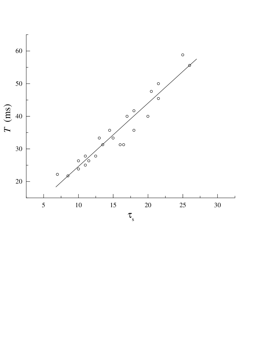
Figure 3: Plot of period vs. synaptic decay time for a hippocampal slice showing linear behavior indicative of the phasic regime. Responses were recorded from inhibitory neurons evoked by glutamate application during a wash-in of 2 $\mu$M pentobarbital (Whittington et al., 1995). Experimental data is provided courtesy of J. Jefferys.

References

- Abbott and van Vreeswijk (1993) Abbott L, and van Vreeswijk C. Asynchronous states in networks of pulse-coupled oscillators. Phys. Rev. E 48:1483-1490.
- Bragin et al. (1995) Bragin A, Jandó G, Nádasdy Z, Hetke J, Wise K, and Buzsáki G. (1995) Gamma (40-100 Hz) oscillation in the hippocampus of the behaving rat. J. Neuroscience 15:47-60.
- Buzsáki (1986) Buzsáki G. (1986) Hippocampal sharp waves: their origin and significance. Brain Res. 398:242-252.
- Chow (1998) Chow CC. Phase-locking in weakly heterogeneous neuronal networks. Physica D (in press).
- Destexhe et al. (1993) Destexhe A, McCormick DA and Sejnowski TJ. (1993) A model for 8-10 Hz spindling in interconnected thalamic relay and reticularis neurons. Biophysical J. 65:2473-2477.
- Destexhe et al. (1994) Destexhe A, Mainen ZF and Sejnowski TJ. (1994) An efficient method for computing synaptic conductances based on a kinetic model of receptor binding. Neural Comp. 6:14-18.
- Ermentrout (1996) Ermentrout GB. (1996) Type I membranes, phase resetting curves, and synchrony. Neural Comp. 8:979-1001.
- Ermentrout and Kopell (1998) Ermentrout GB and Kopell N. (1998) Fine structure of neural spiking and synchronization in the presence of conduction delays. Proc. Nat. Acad. Sci. USA 95:1259-1264.
- Friesen (1994) Friesen W. (1994) Reciprocal inhibition, a mechanism underlying oscillatory animal movements. Neurosci Behavior 18:547-553.
- Gerstner et al. (1996) Gerstner W, van Hemmen JL, and Cowen J. (1996) What matters in neuronal locking? Neural Comp. 8:1653-1676.
- Golomb and Rinzel (1993) Golomb D and Rinzel J. (1993) Dynamics of globally coupled inhibitory neurons with heterogeneity. Phys. Rev. E 48, 4810-4814.
- Gray (1994) Gray CM. (1994) Synchronous oscillations in neuronal systems: mechanisms and functions. J. Comp. Neuro. 1:11-38.
- Hansel et al. (1995) Hansel D, Mato G, and Meunier C. (1995) Synchrony in excitatory neural networks. Neural Comp. 7:307-337.
- Izhikevich and Hoppensteadt (1997) Izhikevich EM. and Hoppensteadt F. Weakly Connected Neural Networks, (Springer-Verlag, 1997, Chapter 8).
- Jefferys et al. (1996) Jefferys JGR, Traub RD, and Whittington MA. (1996) Neuronal networks for induced ‘40 Hz’ rhythms. Trends Neurosci. 19:202-207.
- Katsumaru et al. (1988) Katsumaru H, Kosaka T, Heizman CW, and Hama K. (1988) Gap-junctions on GABAergic neurons containing the calcium-binding protein parvalbumin in the rat hippocampus (CA1 regions). Exp. Brain Res. 72:363-370.
- Kopell and LeMasson (1994) Kopell N. and LeMasson G. (1994) Rhythmogenesis, amplitude modulation, and multiplexing in a cortical architecture. Proc. Natl. Acad. Sci. USA 91:10586-10590.
- Llinás and Ribary (1993) Llinás R and Ribary U. (1993) Coherent 40-Hz oscillation characterizes dream state in humans. Proc. Natl. Acad. Sci. USA 90:2078-2081.
- Perkel and Mulloney (1974) Perkel D and Mulloney B. (1974) Motor patterns in reciprocally inhibitory neurons exhibiting postinhibitory rebound. Science 185:181-183.
- Pinsky and Rinzel (1994) Pinsky P and Rinzel J. (1994) Intrinsic and network rhythmogenesis in a reduced Traub model for CA3 neurons. J. Comp. Neurosci. 1:39-60.
- Rinzel and Ermentrout (1989) Rinzel and Ermentrout, in Methods in Neuronal Modelling, edited by C. Koch and I. Segev (MIT Press, Cambridge, 1989).
- Ritz and Sejnowski (1997) Ritz R and Sejnowski TJ. (1997) Synchronous oscillatory activity in sensory systems: new vistas on mechanisms. Curr. Opin. Neurobio. 7:536-546.
- Skinner et al. (1993) Skinner F, Turrigiano GG, and Marder E. (1993) Frequency and burst duration in oscillating neurons and two-cell networks. Biol. Cybern. 69:375-383.
- Skinner et al. (1994) Skinner F, Kopell N, and Marder E. (1994) Mechanisms for oscillations and frequency control in networks of mutually inhibitory relaxation oscillators. J. Comp. Neurosci. 1:69-87.
- Terman et al. (1996) Terman D, Bose A, and Kopell N. (1996) Functional reorganization in thalamocortical networks: transition between spindling and delta sleep rhythms. Proc. Natl. Acad. Sci. USA 93:15417-15422.
- Terman et al. (1997) Terman, D., Kopell N. and Bose A. Dynamics of two mutually coupled slow inhibitory neurons. Physica D (in press).
- Tuckwell (1989) Tuckwell HC (1989) Stochastic processes in the neurosciences (SIAM, Philadelphia).
- Traub (1995) Traub RD. (1995) Model of synchronized population bursts in electrically coupled interneurons containing active dendritic conductances. J. Comp. Neurosci. 2:283-289.
- Traub et al. (1996a) Traub RD, Whittington M, Colling S, Buzsáki G, and Jefferys JGR. (1996a) Analysis of gamma rhythms in the rat hippocampus in vitro and in vivo. J. Physiol. 493:471-484.
- Traub et al. (1996b) Traub RD, Jefferys JGR, and Whittington MA. (1996b) Simulation of gamma rhythms in networks of interneurons and pyramidal cells. J. Comp. Neurosci. In press.
- Tsodyks et al. (1993) Tsodyks M, Mitkov I, and Sompolinsky, H. (1993) Pattern of synchrony in inhomogeneous networks of oscillators with pulse interactions. Phys. Rev. Lett. 71:1280-1283.
- van Vreeswijk et al. (1994) van Vreeswijk C, Abbott L, and Ermentrout GB. (1994) When inhibition not excitation synchronizes neural firing. J. Comp. Neuroscience 1:313-321.
- Wang and Buzsáki (1996) Wang X-J and Buzsáki G. (1996) Gamma oscillation by synaptic inhibition in an interneuronal network model. J. Neurosci. 16:6402-6413.
- Wang and Rinzel (1992) Wang X-J and Rinzel J. (1992) Alternating and synchronous rhythms in reciprocally inhibitory model neurons. Neural Comp. 4:84-97.
- Whittington et al. (1995) Whittington MA, Traub RD, and Jefferys JGR. (1995) Synchronized oscillations in interneuron networks driven by metabotropic glutamate receptor activation. Nature 373:612-615.
- White et al. (1998) White JA, Chow CC, Ritt J, Soto-Treviño C, and Kopell N. (1998) Synchronization and oscillatory dynamics in heterogeneous, mutually inhibited neurons. J. Comp. Neurosci. (in press).
- Ylinen et al. (1995) Ylinen A, Bragin A, Nádasdy Z, Jandó G, Szabó I, Sik A, and Buzsáki G. (1995) Sharp wave-associated high-frequency oscillation (200 Hz) in the intact hippocampus: network and intracellular mechanisms. J. Neurosci. 15:30-46.