Dynamic Fitness Landscapes in Molecular Evolution

Abstract

We study self-replicating molecules under externally varying conditions. Changing conditions such as temperature variations and/or alterations in the environment’s resource composition lead to both non-constant replication and decay rates of the molecules. In general, therefore, molecular evolution takes place in a dynamic rather than a static fitness landscape. We incorporate dynamic replication and decay rates into the standard quasispecies theory of molecular evolution, and show that for periodic time-dependencies, a system of evolving molecules enters a limit cycle for $t\rightarrow\infty$. For fast periodic changes, we show that molecules adapt to the time-averaged fitness landscape, whereas for slow changes they track the variations in the landscape arbitrarily closely. We derive a general approximation method that allows us to calculate the attractor of time-periodic landscapes, and demonstrate using several examples that the results of the approximation and the limiting cases of very slow and very fast changes are in perfect agreement. We also discuss landscapes with arbitrary time dependencies, and show that very fast changes again lead to a system that adapts to the time-averaged landscape. Finally, we analyze the dynamics of a finite population of molecules in a dynamic landscape, and discuss its relation to the infinite population limit.

and

1 Introduction

Eigen’s quasispecies model [1] has been the basis of a vivid branch of molecular evolution theory ever since it has been put forward almost 30 years ago [2, 3, 4, 5, 6, 7, 8, 9, 10, 11, 12, 13, 14, 15, 16, 17, 18, 19]. Its two main statements are the formation of a quasispecies consisting of several molecular species with well defined concentrations, and the existence of an error threshold above which all information is lost because of accumulating erroneous mutations. Both effects have been found in a number of experimental as well as theoretical studies (For experimental evidence, see, e.g., [20] for the formation of a quasispecies in the RNA of the Q$\beta$ phage, [21] for the observation of an error threshold in a system of self-replicating computer programs, and [22] for a more recent example of quasispecies formation in the Hepatitis C virus. Generally, see the reviews [11, 13, 19] and the references therein). Recently, a new aspect of the quasispecies model has been brought into consideration that was mostly missing in previous works, namely the aspect of a dynamic fitness landscape [17, 18, 23, 24, 25] The notion “Dynamic fitness landscape” encompasses all situations in which the replication and/or decay rates of the molecules change over time. In the present work, we are interested in situations where these changes occur as an external influence for the evolving system, without feedback from the system to the dynamics of the landscape. Dynamic fitness landscapes of this kind are important, because almost any biological system is subject to external changes in the form of, e.g., daytime/nighttime, seasons, long-term climatic changes, geographic changes due to tectonic movements, to name just a few.

The main problem one encounters when dealing with dynamic landscapes is the difficulty to find a good generalization of the quasispecies concept. In the original work of Eigen, the quasispecies is the equilibrium distribution of the different molecular species. It is reached if the system is left undisturbed for a sufficiently long time. Since in a dynamic landscape the system is being disturbed by the landscape itself, the concept of a quasispecies is meaningless in the general case. However, there are special cases in which a meaningful quasispecies can be defined. If, for example, the landscape changes on a much slower time scale than what the system needs to reach the equilibrium, then the system is virtually in equilibrium all the time, and the concentrations at time $t$ are determined from the landscape present at that time. Generally, it is certain symmetries in the dynamics of the landscape that allow for the definition of a quasispecies. One example we treat in this paper in detail is the case of time-periodic landscapes, which offer a natural quasispecies definition.

An early investigation of dynamic landscapes has been carried out by Jones [4, 5], who has only considered cases in which all replication rates change by a common factor. Therefore, this approach excludes (among other cases) in particular all situations in which the order of the molecules’ replication rates changes over time, i.e., in which for example one of the faster replicating molecules becomes one of the slower replicating molecules and vice versa. Recent work on dynamic fitness landscapes allow for such changes. Wilke et al. [26, 17] have developed a framework that allows to define and to calculate numerically a quasispecies in time-periodic landscapes. Independently, Nilsson and Snoad [18] have studied the particular example of a stochastically jumping peak in an otherwise flat landscape. This work has been generalized by Ronnewinkel et al. [23], who could also define a meaningful quasispecies for a deterministic version of the jumping peak landscape and related landscapes. Very recent work of Nilsson and Snoad deals with self-adaptation of the mutation rate in a jumping peak landscape [25], and with the low-pass filter effect of dynamic fitness landscapes [24], a notion put forward by Hirst [27, 28]. Finally, theoretical studies of dynamic fitness landscapes can also be found in the related field of genetic algorithms. Schmitt et al. [29, 30] derive results for finite populations in a relatively broad class of dynamic landscapes. However, only landscapes in which the fitnesses get scaled can be treated, so that the same restriction applies here that applied to Jones’s work. The order of the fitnesses can never change. Also, genetic algorithms with time-periodic landscapes have been studied by Rowe [31, 32]. However, Rowe’s approach has the disadvantage that it is tightly connected to the discrete time used in genetic algorithms, and that the dimension of the transition matrices grows in proportion to the period length $T$ of the oscillation. This makes it hard to derive analytical results, and in addition to that, it renders landscapes with large $T$ inaccessible to numerical calculations.

In this report, we do not cover the large field of molecular evolution in the particular landscapes induced by RNA sequence-to-structure mappings [33, 34, 35], and, in connection to that, we do not discuss neutral networks [36, 37, 38, 39]. We do so mainly because these topics have so far not been studied in the light of temporal variations in the fitness landscapes, and hence, a discussion of them does not fit very well into the general tenor of this work. In general, it can be argued that neutral networks are of less importance in a dynamic environment, because in that situation a population is constantly on the move to the next local optimum [40].

The remainder of this report is structured as follows. We begin our discussion in Section 2.2 with a brief summary of the general aspects of dynamic fitness landscapes in the quasispecies model. In Section 3, we will develop the main subject of this work: a general theory of time-periodic fitness landscapes. The theoretical part thereof is presented in Section 3.1, in which we demonstrate how a time-dependent quasispecies can be defined by means of the monodromy matrix, and how this monodromy matrix can be expanded in terms of the oscillation period $T$. In Section 3.2, we present an alternative approximation formula for the monodromy matrix that is more suitable for numerical calculations, and in Section 3.3, we compare, for several example landscapes, the results obtained from that formula with the general theory developed in Section 3.1. The restriction of a time-periodic fitness landscape is weakened in Section 4, where we discuss the implications of our findings for other, non-periodic fitness landscapes. Since our work is based on Eigen’s deterministic approach with differential equations, all results presented up to the end of Section 4 are only valid for infinite population sizes. In order to address this shortcoming, in Section 5 we give a brief introduction into the problems involved when dealing with finite populations. In Section 5.1, some simulation results are shown, demonstrating the relationship between the results from the infinite population limit and the actual finite population dynamics. Finally, an approximative analytical description of a finite population evolving on a simple periodic landscape is developed in Section 5.2. We close this paper with some conclusions in Section 6.

2 The quasispecies model

2.1 Static landscapes

With his model of self-replicating molecules, Eigen showed for the first time that Darwin’s idea of mutation and selection can work in a simple, seemingly “lifeless” system of chemical reactants. His observation that evolution is governed by the laws of physics spawned a fruitful field of work, and hundreds of papers based on his initial ideas have been written since then. Most of that work has been concerned with static fitness landscapes. There exist comprehensive reviews of that work (see [11, 13] for a very detailed coverage of the literature till 1989, and [19] for a more recent review). Here, we are going to briefly introduce the main concepts developed for static landscapes. In doing so, we restrict ourselves to those concepts that we will refer to later on in our discussion of dynamic fitness landscapes. For a more in-depth discussion of static landscapes, the reader is referred to the above mentioned reviews.

The quasispecies model was originally aimed at describing self-replicating DNA or RNA molecules. Therefore, the molecules were conceived of as sequences consisting of a limited number of elementary building blocks. With that picture in mind, we may represent the molecules as sequences of letters. For RNA molecules, e.g., the conventional alphabet consists of the 4 letters G, A, C, U, representing the 4 bases guanine, adenine, cytosine, and uracil, respectively. Today, most researchers are interested in the information-theoretic aspects of the model. Consequently, the most common alphabet in the molecular evolution literature has become the binary alphabet, consisting of the letters 0 and 1. Throughout this work, we will also adopt this choice. With regard to the RNA example, the binary alphabet can be considered as distinguishing only between purines (which are guanine and adenine) and pyrimidines (which are cytosine and uracil).

The molecules the model describes have the ability to self-replicate. Self-replication is a complicated process, which consumes energy and substrates from the environment. These external resources are supposed to be present, and are not modeled explicitly. The degree to which a macromolecule finds the resources necessary to self-replicate, and is able to exploit them, is expressed in the replication coefficients $A_{i}$. A molecule $i$ that finds good conditions for self-replication has a high $A_{i}$, another molecule $j$ which is a bad self-replicator has a much smaller $A_{j}$.

The molecules replicate by copying themselves. The copy procedure is generally not error-free. Among the different types of errors one can imagine for the copy of a sequence of letters (substitutions, insertions, deletions), we consider only substitutions. Substitutions can in principle occur with a different probability at every single position in the sequence. However, if we assume the copy procedure to be performed step by step by some sort of molecular machinery, the probability of copying a symbol incorrectly can be expected to be the same for all positions in the sequence. Hence, a letter will change from 0 to 1 or vice versa during the copy procedure with a fixed probability, denoted by $R$. This probability is called the error rate, or, alternatively, the mutation rate.

Molecules are also subject to decay with a particular rate $D_{i}$ for species $i$. A molecule that decays is assumed to be completely absorbed by the environment, i.e., it does not break into parts that are themselves being described by the model.

The constant production of new molecules due to the ongoing self-replication will drastically increase the concentration of molecules, and will decrease the amount of resources available for further self-replication. We are interested in the description of a steady state, and therefore we have to introduce a constant dilution which lets new resources enter the system and washes away the excess production of those molecules. The total concentration of molecules can thus be kept constant by proper adjustment of the dilution flux.

Finally, we assume that the self-replicating molecules are placed in a well-stirred reactor. As a consequence of this assumption, we can neglect any spatial correlations in the model, and concentrate solely on the molecules’ abundances.

In summary, the model is based on the following postulates:

1. The molecules are represented by binary sequences of length $l$. They form and decompose steadily. The number of copies of sequence $i$ present at time $t$ is denoted by $n_{i}(t)$.

2. Sequences enter the system solely as the result of a correct or erroneous copy of another sequence already present.

3. The substrates necessary for the ongoing replication are always present in sufficient quantity. Excess molecules are washed away by a flux $\Phi(t)$.

4. The decay of sequences is a Poisson process.

These four assumptions form the basis of Eigen’s theory of molecular evolution. A quantitative analysis of these assumptions can be done in terms of differential equations in the molecules’ occupation numbers $n_{i}(t)$. In the following paragraphs, we recall the quantitative analysis of the model that has been developed by Eigen and coworkers.

We begin by writing down an expression for the change in the number of copies of sequence $i$. The abundance $n_{i}(t)$ of sequence $i$ increases because a proportion of the molecules of type $i$ replicates faithfully, while some of the other molecules of other types produce offspring of type $i$ as the outcome of fruitless attempts to self-replicate. Let the matrix ${\mbox{Q}}=\big{(}Q_{ij}\big{)}$ express the probability that molecule $j$ copies into molecule $i$. The associated increase in the abundance $n_{i}(t)$ then amounts to $\sum_{j}A_{j}Q_{ij}n_{j}(t)$.

The decrease of a molecule’s abundance can have two reasons: its decay, expressed by $-D_{i}n_{i}(t)$, and its removal due to the flux term, expressed by $-n_{i}(t)\Phi(t)/N(t)$. Here, $N(t)$ is the total number of molecules at time $t$, i.e., $N(t)=\sum_{j}n_{j}(t)$. Putting all the different terms together, we end up with the net change $\dot{n}_{i}(t)$ in the number of copies of sequence $i$,

$$\dot{n}_{i}(t)=\Big{[}A_{i}Q_{ii}-D_{i}\Big{]}n_{i}(t)+\sum_{j\neq i}A_{j}Q_{ij}n_{j}(t)-\frac{n_{i}(t)}{N(t)}\Phi(t)\,.$$ (1)

The quantity $Q_{ii}$ gives the probability that a molecule $i$ replicates faithfully. $Q_{ii}$ is sometimes referred to as the copy fidelity.

For the further development of the theory, it is useful to introduce an average excess production $\bar{E}(t)$, defined by

$$\bar{E}(t):=\sum_{i}n_{i}(t)\Big{[}A_{i}-D_{i}\Big{]}\Big{/}N(t)\,.$$ (2)

The conservation law

$$\sum_{i}Q_{ij}=1\,,$$ (3)

expressing the fact that every (possibly erroneous) copy of a molecule represents another molecule in the chemistry, allows us to rewrite the average excess production in terms of the total production rate and the dilution flux, viz.

$$\bar{E}(t)=\left[\sum_{i}\dot{n}_{i}(t)+\Phi(t)\right]\Big{/}N(t)\,.$$ (4)

It proves to be useful to define the matrix ${\mbox{W}}=\big{(}W_{ij}\big{)}$ as

$$W_{ij}:=A_{j}Q_{ij}-D_{i}\delta_{ij}\,.$$ (5)

Now we can rewrite Eq. (1) as

$$\dot{n}_{i}(t)=\Big{[}W_{ii}-\bar{E}(t)\Big{]}n_{i}(t)+\sum_{j\neq i}W_{ij}n_{j}(t)+n_{i}(t)\frac{\dot{N}(t)}{N(t)}\,.$$ (6)

Let us introduce concentration variables $x_{i}(t)$, defined by

$$x_{i}(t):=\frac{n_{i}(t)}{N(t)}\,.$$ (7)

The quantity $x_{i}(t)$ measures the relative concentration of molecule $i$ in the population. The change in $x_{i}(t)$ is given by

$$\dot{x}_{i}(t)=\frac{\dot{n}_{i}(t)}{N(t)}-n_{i}(t)\frac{\dot{N}(t)}{N(t)^{2}}\,.$$ (8)

Hence, if we subtract the rightmost term of Eq. (6) on both sides of Eq. (6), and divide by $N(t)$, we arrive at

$$\dot{x}_{i}(t)=\Big{[}W_{ii}-\bar{E}(t)\Big{]}x_{i}(t)+\sum_{j\neq i}W_{ij}(t)x_{j}(t)\,.$$ (9)

The total number of molecules grows with

$$\dot{N}(t)=\bar{E}(t)N(t)-\Phi(t)\,.$$ (10)

Typically, one assumes that the flux $\Phi(t)$ is adjusted such that $\dot{N}(t)$ vanishes, as expressed by Assumption 3 on page 3. However, this assumption is not really necessary for the further development of the theory. Since from this point onwards, we will only be concerned with the relative concentrations $x_{i}(t)$, we will disregard the flux altogether, and work with Eq. (9) exclusively.

At this point, it is useful to introduce vector notation, by lumping the concentrations $x_{1}(t),x_{2}(t),\dots$ together into a single vector $\mbox{\boldmath$x$}(t)=\big{(}x_{1}(t),x_{2}(t),\dots\big{)}$. Equation (9) then becomes

$$\dot{\mbox{\boldmath$x$}}(t)=\Big{[}{\mbox{W}}-\bar{E}(t)\mbox{\boldmath$1$}\Big{]}\mbox{\boldmath$x$}(t),$$ (11)

where $1$ is the identity matrix. The matrix W can be decomposed into

$${\mbox{W}}={\mbox{Q}}{\mbox{A}}-{\mbox{D}}\,,$$ (12)

if we write the replication and the decay coefficients in matrix form as well. Both A and D are diagonal matrices of the form

A $$={\rm diag}\left(A_{1},A_{2},\dots\right)\,,$$ (13a)

D $$={\rm diag}\left(D_{1},D_{2},\dots\right)\,.$$ (13b)

The matrix Q is the mutation matrix introduced above. Note that the average excess production can also be transformed into vector notation. It takes on the form

$$\overline{E}(t)=\mbox{\boldmath$e$}^{\rm t}\cdot[{\mbox{A}}(t)\mbox{\boldmath$x$}(t)-{\mbox{D}}(t)\mbox{\boldmath$x$}(t)]\,,$$ (14)

where $\mbox{\boldmath$e$}^{\rm t}$ is a vector of 1s, i.e., $\mbox{\boldmath$e$}^{\rm t}=(1,\dots,1)$. The scalar product between $\mbox{\boldmath$e$}^{t}$ and a concentration vector [say $\mbox{\boldmath$y$}(t)$] gives exactly the sum over all components of that vector.

Equation (11) is nonlinear, since the term $\bar{E}(t)\mbox{\boldmath$x$}(t)$ is quadratic in $\mbox{\boldmath$x$}(t)$. Nevertheless, a straightforward solution of Eq (11) is possible, because a transformation exists which removes the nonlinearity. The strength of this transformation lies in the easy reconstruction of the concentration variables $x_{i}(t)$ from the transformed system. Following Thompson and McBride [2], or Jones et al. [3], we introduce

$$\mbox{\boldmath$y$}(t):=\exp\left(\int_{0}^{t}\bar{E}(\tau)\,d\tau\right)\mbox{\boldmath$x$}(t)\,.$$ (15)

The new variables satisfy the linear equation

$$\dot{\mbox{\boldmath$y$}}(t)={\mbox{W}}\mbox{\boldmath$y$}(t)\,,$$ (16)

which can be shown by insertion of Eq. (15) into Eq. (16). Moreover, since $\mbox{\boldmath$y$}(t)$ differs from $\mbox{\boldmath$x$}(t)$ only by a scalar factor, we can restore the original variables via

$$\mbox{\boldmath$x$}(t)=\frac{\mbox{\boldmath$y$}(t)}{\mbox{\boldmath$e$}^{\rm t}\cdot\mbox{\boldmath$y$}(t)}\,.$$ (17)

Note that if all decay constants are equal, i.e., ${\mbox{D}}={\rm diag}(D,\dots,D)$ with a single scalar value $D$, then the transformation

$$\mbox{\boldmath$y$}(t)=\exp\left(\int_{0}^{t}[\overline{E}(\tau)+D]\,d\tau\right)\mbox{\boldmath$x$}(t)$$ (18)

leads to the even simpler equation

$$\dot{\mbox{\boldmath$y$}}(t)={\mbox{Q}}{\mbox{A}}\mbox{\boldmath$y$}(t)\,.$$ (19)

The concentration vector $\mbox{\boldmath$x$}(t)$ can again be obtained from Eq. (17).

The mutation matrix Q has so far remained undefined. The choice of Q specifies the relationship between the different molecules in the chemistry. As was stated above, we conceive the molecules as bitstrings of length $l$, and we assume that copy errors are equally likely on all positions on the string. In that case, the mutation matrix can be written down straightforwardly. Suppose that two bitstrings differ in $d$ positions. A mutation from one to the other occurs only if exactly these $d$ positions are copied erroneously, while all others are copied faithfully. Such a copy error appears with probability $(1-R)^{l-d}R^{d}$. Hence, we can write the mutation matrix Q as

$$Q_{ij}=(1-R)^{l}\left(\frac{R}{1-R}\right)^{d(i,j)},$$ (20)

where $d(i,j)$ is the Hamming distance between two sequences. The Hamming distance is the number of bits in which two sequences differ.

The matrix Q is typically very large, since its number of rows and columns grows as $2^{l}$ with increasing sequence length $l$. This makes Eq. (16) almost intractable, numerically as well as analytically, for all but the shortest sequences. An alternative matrix ${\mbox{Q}}^{\prime}$ is often used, in which certain sequences are grouped together, such that the number of concentration variables can be reduced to $l+1$. The main idea of this grouping, developed by Swetina and Schuster [7], is to define a single sequence (which should have the highest replication coefficient of all sequences) as master sequence, and to group all other sequences into error classes, according to their Hamming distance from the chosen master sequence. All the sequences with the same Hamming distance from the master form a single error class. This procedure has the advantage of greatly reducing the number of variables, but it also restricts considerably the number of fitness landscapes that can be studied. Since all sequences in an error class have to share the same replication coefficient, a fitness landscape, for example, in which two peaks have a small or moderately large Hamming distance cannot be defined.

The error class matrix ${\mbox{Q}}^{\prime}$ has been given by Nowak and Schuster [14] in a relatively simple form:

$$Q^{\prime}_{ij}=\sum_{k=\max\{i+j-l,0\}}^{\min\{i,j\}}\binom{j}{k}\binom{l-j}{i-k}(1-R)^{l}\left(\frac{R}{1-R}\right)^{i+j-2k}\,.$$ (21)

Note that in [14], the indices $i$ and $j$ are interchanged inadvertently. The error class matrix can be derived from Eq. (20) by deletion of all but one column of every group of columns whose index $j$ yields the same $d(0,j)$, and by the subsequent summation of all rows whose index $i$ yields the same $d(i,0)$.

The linearized evolution equation (16) can be solved analytically. The transition from an initial state $\mbox{\boldmath$y$}(0)$ to the state at time $t$ is given by [41]

$$\mbox{\boldmath$y$}(t)=\exp({\mbox{W}}t)\mbox{\boldmath$y$}(0)\,.$$ (22)

From that expression, we can read off that the (unnormalized) variables $\mbox{\boldmath$y$}(t)$ will grow exponentially over time. Mathematically, this growth can be accompanied by either exponentially damped or exponentially amplified oscillations. For all cases of biological interest, however, there can be at most exponentially damped oscillations. First of all, we will almost always deal with a symmetric matrix Q. A symmetric mutation matrix implies that the probability with which a sequence $i$ mutates into a sequence $j$ is the same as the probability for the inverse process. Rumschitzki has noted that in this case, the spectrum of W is real [9]. Namely, we can transform the non-symmetric matrix W into a symmetric one by means of a similarity transformation,

$${\mbox{W}}={\mbox{Q}}{\mbox{A}}-{\mbox{D}}\quad\rightarrow\quad{\mbox{A}}^{1/2}{\mbox{W}}{\mbox{A}}^{-1/2}={\mbox{A}}^{1/2}{\mbox{Q}}{\mbox{A}}^{1/2}-{\mbox{D}}\,.$$ (23)

The spectrum of the transformed matrix is real because of the matrix’s symmetry, and hence the spectrum of the untransformed matrix must be real as well. In that case, oscillations will be absent in Eq. (22). For non-symmetric Q, we can apply the Frobenius-Perron theorem [42] if the decay rates satisfy

$$({\mbox{D}})_{ii}<({\mbox{Q}}{\mbox{A}})_{ii}\qquad\mbox{for all $i$.}$$ (24)

The Frobenius-Perron theorem is applicable to a matrix with all positive entries, and it guarantees a real largest eigenvalue for that matrix. Consequently, we have at most exponentially damped oscillations as long as (24) is obeyed. In addition to that, the Frobenius-Perron theorem states that the eigenvector corresponding to this largest eigenvalue has only strictly positive entries, and hence, that this eigenvector can be interpreted as a vector of chemical concentrations if normalized appropriately.

Let us write down a more explicit solution to (16), under the assumption that the spectrum of W is known (exact spectra of evolution matrices have been derived in [9, 43, 44]). Let $\lambda_{k}$ be the eigenvalues of W, and let $\mbox{\boldmath$\phi$}_{k}$ be the associated eigenvectors. Without loss of generality, we order the eigenvalues such that $\lambda_{0}\geq\lambda_{1}\geq\lambda_{2}\geq\dots$ . The solution to Eq. (16) can then be expressed as

$$\mbox{\boldmath$y$}(t)=\sum_{k}\alpha_{k}\mbox{\boldmath$\phi$}_{k}\,e^{\lambda_{k}t}\,,$$ (25)

where the coefficients $\alpha_{k}$ have to be chosen such that the initial condition $\mbox{\boldmath$y$}(t=0)=:\mbox{\boldmath$y$}_{0}$ is satisfied. In other words, the $\alpha_{k}$ give the expansion of the initial condition $\mbox{\boldmath$y$}_{0}$ in terms of the eigenvectors $\mbox{\boldmath$\phi$}_{k}$,

$$\mbox{\boldmath$y$}_{0}=\sum_{k}\alpha_{k}\mbox{\boldmath$\phi$}_{k}\,.$$ (26)

The principal eigenvector $\mbox{\boldmath$\phi$}_{0}$ of W has been called the quasispecies by Eigen. The reason for this name will become clear shortly.

In terms of the concentration variables $\mbox{\boldmath$x$}(t)$, the solution Eq. (25) becomes

$$\mbox{\boldmath$x$}(t)=\frac{\mbox{\boldmath$y$}(t)}{\mbox{\boldmath$e$}^{\rm t}\cdot\mbox{\boldmath$y$}(t)}\,,$$ (27)

where $e$ is again a vector with all entries equal to 1.

As we already mentioned, the Perron-Frobenius theorem assures that the largest eigenvalue $\lambda_{0}$ is non-degenerate, and that all components of the corresponding eigenvector $\mbox{\boldmath$\phi$}_{0}$ are positive. We factor out the exponential of the largest eigenvalue $e^{\lambda_{0}t}$ in the numerator and denominator of Eq. (27) and obtain

$$\mbox{\boldmath$x$}(t)=\frac{\alpha_{0}\mbox{\boldmath$\phi$}_{0}+\sum_{k>0}\alpha_{k}\mbox{\boldmath$\phi$}_{k}\,e^{(\lambda_{k}-\lambda_{0})t}}{\sum_{k}\alpha_{k}\,\mbox{\boldmath$e$}\cdot\mbox{\boldmath$\phi$}_{k}\,e^{(\lambda_{k}-\lambda_{0})t}}\,.$$ (28)

As long as $\alpha_{0}\neq 0$, all contributions apart from the one corresponding to the largest eigenvalue disappear in the limit $t\rightarrow\infty$. Hence, the system evolves towards a steady state, characterized by the dominant eigenvector of the matrix W.

The case $\alpha_{0}=0$ is somewhat artificial, because it implies that the system has been started in an exact superposition of eigenstates excluding the dominant quasispecies. In that case, the system cannot evolve towards $\mbox{\boldmath$\phi$}_{0}$. Instead, it converges towards the eigenvector corresponding to the next-largest eigenvalue. In a real chemical system with more or less random initial conditions and under the presence of noise, the case $\alpha_{0}=0$ is of no relevance.

The appearance of a steady state distribution of concentration variables has important implications for the understanding of Darwinian evolution. In general, the eigenvectors $\mbox{\boldmath$\phi$}_{k}$ are a mixture of several molecular species $i$. As a consequence, a number of species is present simultaneously in the asymptotic distribution. This means that selection combined with random mutation does not remove all but one molecular species, even if there exists one (the master sequence) whose replication coefficient exceeds all others. Instead, the interplay of selection and mutation creates a cloud of mutant species around the master sequence. It is this cloud that is termed the quasispecies. The mutant distribution forms a unit competing with other similar units, represented by the other eigenvectors. Selection acts on these mixtures of sequences, and ultimately singles out the dominant one, i.e., the one corresponding to the largest eigenvalue.

Figure 1: The relative concentrations of the master sequence and the error classes for sequences of length $l=20$ versus the error rate $R$ in a sharply peaked landscape with replication coefficients $A_{0}=10,A_{1},\dots,A_{20}=1$. The concentrations of all sequences with the same distance $d$ to the master are summed up and displayed as a single line. The decay constants have been set to $D_{i}=D$, with arbitrary $D$. In static fitness landscapes, the decay constants drop out of the asymptotic quasispecies if they are all equal.

Interestingly, the master sequence does not necessarily occupy a large fraction of the quasispecies. In fact, as the mutation rate increases, it is common that the master dwindles while the one-mutant and the two-mutant sequences form the prevailing part of the quasispecies. Figure 1 shows the asymptotic sequence distribution versus the error rate $R$ for a sharply peaked landscape in which all but one of the replication coefficients are identical, while the remaining one exceeds them significantly. The mutants are grouped into error classes. If copy errors are not present, i.e., for $R=0$, the master sequence is the only species present, and all others have a vanishing concentration. As soon as $R$ takes on values slightly above 0, the concentration of the master sequence starts to decrease. At the same time, the concentrations of the mutants begin to grow, first that of the one-mutant sequence, than that of the two-mutant sequence, and so on. At $R=0.11$ we observe a sharp transition, beyond which the concentrations take on constant values. The mutation rate at which this transition occurs is called the error threshold. Beyond the error threshold, the outcome of a replication event can be considered a random sequence, and therefore, all molecular species take on the same concentration in this regime. The fact that all concentrations are equal beyond the error threshold is somewhat blurred in Fig. 1 because of the use of error classes. In fact, the heights of the different curves merely reflect the sizes of the corresponding error classes. For $R=\frac{1}{2}$, the sequences replicate stochastically in any landscape, since faithfully copied and erroneously copied symbols are then equally likely. The outcome of a single copy process is therefore a random sequence in that case. When $R$ comes close to the value 1, almost every symbol is copied incorrectly. This implies that the copy is, apart from mutations, the inverse of the original sequence (note that this is a peculiarity of binary strings). As a consequence, order can again be seen for large $R$. In Fig. 1, the inverse error threshold occurs at $R=0.94$. Beyond that point, the inverse master sequence dominates the quasispecies.

If an evolving system displays an error threshold, the amount of information that can be acquired by the system is severely limited. In the case of the sharply peaked landscape, the critical mutation rate at which the error threshold occurs decreases as $1-(1/\sigma)^{1/l}$ with increasing string length [45]. The quantity $\sigma$ in that expression stands for the relative advantage of the master sequence over the other sequences. For large $l$, the critical mutation rate is therefore very close to 0. This implies that for a given mutation rate, the molecules can grow to a certain length, while beyond that length, all information is lost. Incidentally, it follows that the spontaneous formation of complex self-replicating molecules seems to be impossible. Eigen and Schuster attempted to solve this problem with the concept of the hypercycle [6]. However, it must be said that not all landscapes do present an error threshold. In particular, multiplicative landscapes [46, 47, 48] show a smooth crossover from the completely ordered situation at $R=0$, where the master sequence is the only sequence present, to $R=\frac{1}{2}$, where all molecules take on the same concentration. Moreover, the decay of the master sequence’s concentration depends only on the mutation rate and the selective advantage, but not on the length of the strings. Hence, in a multiplicative model, sequences can grow in length without bound, and self-replicating molecules might form spontaneously.

The error threshold can be viewed as the critical point of a phase transition. This fact is well established through a rich body of work, in which the quasispecies model and related models have been mapped onto spin lattices [49, 10, 50], spin chains [51, 48], and more recently also onto the statistical mechanics of directed polymers in a random medium [44]. The order parameter that is generally being used to describe that phase transition is the average overlap of the sequences in the population with the master sequence, given by the expression $l-2d(0,i)$, where $d(0,i)$ is the Hamming distance between a sequence of type $i$ and the master sequence. The overlap takes on the value $l$ if we compare the master sequence with itself, the value $-l$ if we compare it with its inverse, and intermediate values for all other sequences. The order parameter reads

$$m_{s}=\frac{1}{l}\sum_{i}x_{i}[l-2d(0,i)]\,.$$ (29)

We use the symbol $m_{s}$ because the order parameter represents the surface magnetization when we map the quasispecies model onto an Ising lattice [10, 50].

2.2 Time-dependent replication rates

Having developed a good understanding of the concepts of molecular evolution theory in static environments, let us move on to the non-static case. The basic quasispecies equation (11) changes only in so far as the matrix W now becomes time dependent,

$$\dot{\mbox{\boldmath$x$}}(t)=[{\mbox{W}}(t)-\overline{E}(t)\mbox{\boldmath$1$}]\mbox{\boldmath$x$}(t)\,.$$ (30)

In the most general case, the time dependency may stem from the replication rates, from the decay rates, or even from the mutation matrix:

$${\mbox{W}}(t)={\mbox{Q}}(t){\mbox{A}}(t)-{\mbox{D}}(t)\,.$$ (31)

The average excess production is then

$$\overline{E}(t)=\mbox{\boldmath$e$}^{\rm t}\cdot[{\mbox{A}}(t)\mbox{\boldmath$x$}(t)-{\mbox{D}}(t)\mbox{\boldmath$x$}(t)]\,.$$ (32)

As in the static case, we can transform away the nonlinearity in Eq. (30) with the introduction of unnormalized variables

$$\mbox{\boldmath$y$}(t)=\exp\left(\int_{0}^{t}\overline{E}(\tau)\,d\tau\right)\mbox{\boldmath$x$}(t)\,.$$ (33)

The resulting equation is again a linear differential equation, however, this time with non-constant coefficients:

$$\dot{\mbox{\boldmath$y$}}(t)={\mbox{W}}(t)\mbox{\boldmath$y$}(t)\,.$$ (34)

As in the static case, if all decay constants are equal, i.e., ${\mbox{D}}(t)={\rm diag}(D(t),\dots,D(t))$ with a single scalar function $D(t)$, then an extended transformation similar to Eq. (18) removes the decay constants from Eq. (34).

In the previous subsection, we were able to immediately write down a solution for the linearized quasispecies equation. In the case of a dynamic fitness landscape, however, no such a simple closed form solution exists. Instead, we have to be satisfied with partial solutions, approximations, and limiting cases. In particular, we cannot generally define a quasispecies as the steady state the system approaches for $t\rightarrow\infty$. Therefore, a central question in relation to dynamic landscapes is the appropriate definition of a quasispecies concept.

For now, we start collecting information about Eq. (34). First of all, we note that we can map the quasispecies model onto a linear system with a symmetric matrix $\tilde{{\mbox{W}}}(t)$ if ${\mbox{Q}}(t)$ is symmetric for all $t$. This can be seen by introducing

$$\mbox{\boldmath$z$}(t)={\mbox{A}}^{1/2}(t)\mbox{\boldmath$y$}(t)\,.$$ (35)

Differentiation yields

$$\dot{\mbox{\boldmath$z$}}(t)=\tilde{{\mbox{W}}}(t)\mbox{\boldmath$z$}(t)$$ (36)

with

$$\tilde{{\mbox{W}}}(t)={\mbox{A}}^{1/2}(t){\mbox{Q}}(t){\mbox{A}}^{1/2}(t)-{\mbox{D}}(t)+\left[\frac{d}{dt}{\mbox{A}}^{1/2}(t)\right]{\mbox{A}}^{-1/2}(t)\,.$$ (37)

Unfortunately, we cannot write down a solution for Eq. (36) from the knowledge of the eigensystem of $\tilde{{\mbox{W}}}(t)$ if $\tilde{{\mbox{W}}}(t)$ has an arbitrary time dependency. However, the above mapping shows that for symmetric ${\mbox{Q}}(t)$, we may safely assume that the matrix ${\mbox{W}}(t)$ has only real eigenvalues.

There are two limiting cases that we can discuss without specifying a landscape, namely very fast changes in ${\mbox{W}}(t)$ on the one hand, and very slow changes in ${\mbox{W}}(t)$ on the other hand. We begin with the case of very slow changes. For the rest of this work, we will assume that ${\mbox{W}}(t)$ has a real spectrum for all $t$. To be on the safe side, we also assume that (24) is satisfied for all $t$. In that way, the Perron eigenvector of ${\mbox{W}}(t)$ can always be interpreted as a vector of chemical concentrations.

For every time $t_{0}$, we can define a relaxation time

$$\tau_{\rm R}(t_{0})=\frac{1}{\lambda_{0}(t_{0})-\lambda_{1}(t_{0})}\,,$$ (38)

where $\lambda_{0}(t)_{0}$ and $\lambda_{1}(t_{0})$ are the largest and the second largest eigenvalue of ${\mbox{W}}(t_{0})$, respectively. The time $\tau_{\rm R}(t_{0})$ gives an estimate of how long a linear system with matrix ${\mbox{W}}(t_{0})$ needs to settle into equilibrium. Therefore, if the changes in ${\mbox{W}}(t)$ happen on a timescale much longer than $\tau_{\rm R}(t)$, the system is virtually in equilibrium at any given point in time. Hence, for large enough $t$, the quasispecies will be given by the Perron eigenvector of ${\mbox{W}}(t)$. Strictly speaking, this is only true if there is always some overlap between the largest eigenvector of ${\mbox{W}}(t)$ and the one of ${\mbox{W}}(t+dt)$, but in all but some very pathological cases we can assume this to be the case.

The situation of fast changes in ${\mbox{W}}(t)$ is somewhat more difficult, because, as we are going to see later on, we have to define a suitable average over ${\mbox{W}}(t)$ in order to make a general statement. Therefore, we postpone this case for a moment. A detailed discussion of fast changes will be given for the particular case of periodic fitness landscapes in the next section, and later on, we will discuss fast changing landscapes in general.

3 Periodic fitness landscapes

3.1 Differential equation formalism

In this section, we study periodic time dependencies in ${\mbox{W}}(t)$, for which we can prove several general statements.

If the changes in ${\mbox{W}}(t)$ are periodic, i.e., if there exists a $T$ such that

$${\mbox{W}}(t+T)={\mbox{W}}(t)\quad\mbox{for all $t$,}$$ (39)

then Eq. (34) turns into a system of linear differential equations with periodic coefficients. Several theorems are known for such systems [52]. Most notably, if ${\mbox{Y}}(t,t_{0})$ is the fundamental matrix, such that every solution to Eq. (34) can be written in the form

$$\mbox{\boldmath$y$}(t)={\mbox{Y}}(t,t_{0})\mbox{\boldmath$y$}(t_{0})\,,$$ (40)

then we can define the monodromy matrix ${\mbox{X}}(t_{0})$,

$${\mbox{X}}(t_{0})={\mbox{Y}}(t_{0}+T,t_{0})\,,$$ (41)

which simplifies Eq. (40) to

$$\mbox{\boldmath$y$}(t) ={\mbox{Y}}(t_{0}+\phi,t_{0}){\mbox{X}}^{m}(t_{0})\mbox{\boldmath$y$}(t_{0})$$

$$={\mbox{X}}^{m}(t_{0}+\phi){\mbox{Y}}(t_{0}+\phi,t_{0})\mbox{\boldmath$y$}(t_{0})\,,$$ (42)

for the decomposition $t=mT+\phi+t_{0}$ with the phase $\phi<T$. In particular, we have

$$\mbox{\boldmath$y$}(\phi+mT)={\mbox{X}}^{m}(\phi)\mbox{\boldmath$y$}(\phi)\,,$$ (43)

so that for every phase $\phi$, we have a well defined asymptotic solution, given by the eigenvector associated with the largest eigenvalue of ${\mbox{X}}(\phi)$. Hence, periodic fitness landscapes allow the definition of a quasispecies, much in the same way as static fitness landscapes do. However, here the quasispecies is time-dependent. In other words, a system that evolves in a periodic fitness landscape runs for $t\rightarrow\infty$ into a limit cycle with period length $T$.

3.1.1 Neumann series for X

With the knowledge of the monodromy matrix X, the calculation of the system’s limit cycle becomes a simple eigenvalue problem. The monodromy matrix, however, can in general not be given in a closed from. Consequently, we have to rely on expansions in various parameters. In this section, we derive a formal expansion in $T$ for the monodromy matrix. This formal expansion is similar in spirit to the Neumann series which gives a formal solution to an integral equation, and it is based on the Picard-Lindelöf iteration for differential equations. As the first step, we have to rewrite Eq. (34) in the form of an integral equation, i.e.,

$$\mbox{\boldmath$y$}(t_{0}+\tau)=\mbox{\boldmath$y$}(t_{0})+\int_{0}^{\tau}{\mbox{W}}(t_{0}+\tau_{1})\mbox{\boldmath$y$}(t_{0}+\tau_{1})d\tau_{1}\,.$$ (44)

Our goal is to solve this equation for $\mbox{\boldmath$y$}(t_{0}+\tau)$ by iteration. Our initial solution is

$$\mbox{\boldmath$y$}_{0}(t_{0}+\tau)=\mbox{\boldmath$y$}(t_{0})\,,$$ (45)

which we insert into Eq. (44). As a result, we obtain the 1st order approximation

$$\mbox{\boldmath$y$}_{1}(t_{0}+\tau)=\mbox{\boldmath$y$}(t_{0})+\int_{0}^{\tau}{\mbox{W}}(t_{0}+\tau_{1})\mbox{\boldmath$y$}(t_{0})d\tau_{1}\,.$$ (46)

Further iteration yields

$$\mbox{\boldmath$y$}_{2}(t_{0}+\tau)=\mbox{\boldmath$y$}(t_{0})+\int_{0}^{\tau}{\mbox{W}}(t_{0}+\tau_{1})\mbox{\boldmath$y$}(t_{0})d\tau_{1}\\ +\int_{0}^{\tau}{\mbox{W}}(t_{0}+\tau_{1})\int_{0}^{\tau_{1}}{\mbox{W}}(t_{0}+\tau_{2})\mbox{\boldmath$y$}(t_{0})d\tau_{1}d\tau_{2}\,,$$ (47)

and so on. Now we define

$$\overline{{\mbox{W}}}_{0}(t_{0},\tau) =1\,,$$ (48)

$$\overline{{\mbox{W}}}_{1}(t_{0},\tau) =\frac{1}{\tau}\int_{0}^{\tau}{\mbox{W}}(t_{0}+\tau_{1})d\tau_{1}\,,$$ (49)

and, in general

$$\overline{{\mbox{W}}}_{k}(t_{0},\tau)=\frac{1}{\tau^{k}}\int_{0}^{\tau}{\mbox{W}}(t_{0}+\tau_{1})\int_{0}^{\tau_{1}}{\mbox{W}}(t_{0}+\tau_{2})\cdots\int_{0}^{\tau_{k}-1}{\mbox{W}}(t_{0}+\tau_{k})d\tau_{1}d\tau_{2}\cdots d\tau_{k}\,,$$ (50)

and obtain the formal solution

$$\mbox{\boldmath$y$}(t_{0}+\tau)=\sum_{k=0}^{\infty}\tau^{k}\overline{{\mbox{W}}}_{k}(t_{0},\tau)\mbox{\boldmath$y$}(t_{0})\,.$$ (51)

For suitably small $\tau$, the infinite sum on the right-hand side is guaranteed to converge. When we compare this equation for $\tau=T$ to the definition of the monodromy matrix Eq. (41), we find that [introducing $\overline{{\mbox{W}}}_{k}(t_{0}):=\overline{{\mbox{W}}}_{k}(t_{0},T)$]

$${\mbox{X}}(t_{0})=\sum_{k=0}^{\infty}T^{k}\overline{{\mbox{W}}}_{k}(t_{0})\,.$$ (52)

In particular, since $\overline{{\mbox{W}}}_{1}(t_{0})$ is identical to the time-average over ${\mbox{W}}(t)$, regardless of $t_{0}$, we have the high-frequency expansion

$${\mbox{X}}(t_{0})=\mbox{\boldmath$1$}+T\overline{{\mbox{W}}}+{\mathcal{O}}(T^{2})\,,$$ (53)

with

$$\overline{{\mbox{W}}}=\frac{1}{T}\int_{0}^{T}{\mbox{W}}(t)\,dt\,.$$ (54)

Equation (53) reveals that for very high frequency oscillations, the system behaves as if it was subject to a static landscape. That static landscape is given by the dynamic landscape’s average over one oscillation period.

The radius of convergence of the expansion Eq. (52) can be estimated as follows. Since all entries of ${\mbox{W}}(t)$ are positive, the tensor

$$\overline{W}_{i\nu_{1}}\overline{W}_{\nu_{1}\nu_{2}}\cdots\overline{W}_{\nu_{k-1}j}(t_{0}) :=\frac{1}{T^{k}}\int_{0}^{T}W_{i\nu_{1}}(t_{0}+\tau_{1})\int_{0}^{\tau_{1}}W_{\nu 1\nu_{2}}(t_{0}+\tau_{2})\cdots$$

$$\qquad\qquad\int_{0}^{\tau_{k-1}}W_{\nu_{k-1}j}(t_{0}+\tau_{k})d\tau_{1}d\tau_{2}\cdots d\tau_{k}$$ (55)

can be bound by

$$\overline{W}_{i\nu_{1}}\overline{W}_{\nu_{1}\nu_{2}}\cdots\overline{W}_{\nu_{k-1}j}(t_{0}) \leq\frac{1}{T^{k}}\int_{0}^{T}W_{i\nu_{1}}(t_{0}+\tau)d\tau\int_{0}^{T}W_{\nu 1\nu_{2}}(t_{0}+\tau)d\tau\cdots$$

$$\qquad\qquad\int_{0}^{T}W_{\nu_{k-1}j}(t_{0}+\tau)d\tau\,,$$ (56)

from which it follows that

$$\left(\overline{{\mbox{W}}}_{k}(t_{0})\right)_{ij}\leq\left(\overline{{\mbox{W}}^{k}}\right)_{ij}\,.$$ (57)

The matrix norm induced by the sum norm

$$\left\|{(y_{1},y_{2},\dots,y_{n})}\right\|_{1}=\sum_{i}|y_{i}|$$ (58)

is the column-sum norm

$$\left\|{\overline{{\mbox{W}}}}\right\|_{1}=\max_{j}\left\{\sum_{i}|\overline{W}_{ij}|\right\}\,.$$ (59)

With that norm, and using Eq. (57), we can estimate

$$\left\|{\overline{{\mbox{W}}}_{k}(t_{0})}\right\|_{1}\leq\left\|{\overline{{\mbox{W}}}^{k}}\right\|_{1}\leq\left\|{\overline{{\mbox{W}}}}\right\|_{1}^{k}\,.$$ (60)

Hence, the expansion Eq. (52) converges certainly for those $T$ that satisfy

$$T\left\|{\overline{{\mbox{W}}}}\right\|_{1}<1\,.$$ (61)

Since all entries in W are positive, we have further

$$\left\|{\overline{{\mbox{W}}}}\right\|_{1} =\max_{j}\left\{\sum_{i}|\overline{A}_{j}Q_{ij}-\overline{D}_{j}\delta_{ij}|\right\}$$

$$=\max_{j}\left\{\overline{A}_{j}-\overline{D}_{j}\right\}\,,$$ (62)

where the bar in $\overline{A}_{j}$ and $\overline{D}_{j}$ indicates that these quantities are averaged over one oscillation period. The second equality holds because of (24) and because of $\sum_{i}{\mbox{Q}}_{ij}=1$. Without loss of generality, we assume that the maximum is given by $\overline{A}_{0}-\overline{D}_{0}$. Then, Eq. (61) is satisfied for

$$T<\frac{1}{\overline{A}_{0}-\overline{D}_{0}}\,.$$ (63)

It is interesting to compare this expression to the relaxation time of the time-averaged fitness landscape, $\overline{\tau}_{\rm R}$. To $0$th order, the principal eigenvalue of $\overline{{\mbox{W}}}$ is given by $\overline{W}_{00}$. The second largest eigenvalue is to the same order given by the second largest diagonal element of $\overline{{\mbox{W}}}$, which we assume to be $\overline{W}_{11}$ without loss of generality. Hence, the relaxation time is approximately given by

$$\overline{\tau}_{\rm R}=\frac{1}{\overline{W}_{00}-\overline{W}_{11}}>\frac{1}{\overline{W}_{00}}\geq\frac{1}{\overline{A}_{0}-\overline{D}_{0}}\,,$$ (64)

which is in general larger than the radius of convergence of Eq. (52). In particular, if the largest and the second largest eigenvalue of $\overline{{\mbox{W}}}$ lie close together, the relaxation time may be much larger than the largest oscillation period for which the expansion is feasible. This restricts the usefulness of Eq. (52) to substantially high frequency oscillations in the landscape. The interesting regime in which the changes in the landscape happen on a time scale comparable to the relaxation time of the system can unfortunately not be studied from Eq. (52).

3.1.2 Exact solutions for $R=0$ and $R=0.5$

The two extreme cases $R=0$ (no replication errors) and $R=0.5$ (random offspring sequences) allow for an exact analytic treatment. The second case is identical to the case of static landscapes, and therefore we will mention it only briefly. At the point of stochastic replication $R=0.5$, the population dynamics becomes independent of the details of the landscape. As a consequence, temporal changes in the landscape must become less important as $R$ approaches $R=0.5$. However, this is not very surprising, since in most cases, an error rate close to 0.5 implies that the population has already passed the error threshold, which in turn implies that it does not feel the changes in the landscape any more.

The case of $R=0$, on the other hand, is more complex than the corresponding case in a static landscape. Since the matrix Q becomes the identity matrix for $R=0$, Eq. (34) reduces to

$$\dot{\mbox{\boldmath$y$}}(t)=[{\mbox{A}}(t)-{\mbox{D}}(t)]\mbox{\boldmath$y$}(t)\,.$$ (65)

The matrices ${\mbox{A}}(t)$ and ${\mbox{D}}(t)$ are diagonal by definition, and hence, a solution to Eq. (65) is given by

$$\mbox{\boldmath$y$}(t)=\exp\left(\int_{t_{0}}^{t}[{\mbox{A}}(t^{\prime})-{\mbox{D}}(t^{\prime})]dt^{\prime}\right)\mbox{\boldmath$y$}(t_{0})\,.$$ (66)

When we compare this expression to Eqs. (40) and (41), we find

$${\mbox{Y}}(t,t_{0})=\exp\left(\int_{t_{0}}^{t}[{\mbox{A}}(t^{\prime})-{\mbox{D}}(t^{\prime})]dt^{\prime}\right)\,,$$ (67)

and, in particular,

$${\mbox{X}}(\phi)=\exp\left(\int^{\phi+T}_{\phi}[{\mbox{A}}(t^{\prime})-{\mbox{D}}(t^{\prime})]dt^{\prime}\right)\,.$$ (68)

The integral in the second expression is taken over a complete oscillation period, and hence, it is independent of $\phi$. Thus, we find for arbitrary $\phi$

$${\mbox{X}}(\phi)=\exp(\overline{{\mbox{W}}})\quad\mbox{for $R=0$.}$$ (69)

With a vanishing error rate, the monodromy matrix becomes the exponential of the time-average over ${\mbox{W}}(t)$. Since the exponential function only affects the eigenvalues of a matrix, the quasispecies is given by the principal eigenvector of $\overline{{\mbox{W}}}$, irrespective of the length of the oscillation period $T$. In other words, in the absence of mutations will the sequence $i$ with the highest average value of $A_{i}(t)-D_{i}(t)$ take over the whole population after a suitable amount of time, provided it existed already in the population at the beginning of the process. By continuity, this property must extend to very small but positive error rates $R$. So, similar to the case of $R=0.5$, the temporal changes in the landscape loose their importance when $R$ approaches 0.

There is, however, a caveat to the above argument. In case the largest eigenvalue of $\overline{{\mbox{W}}}$ is degenerate, temporal changes in the landscape may continue to be of importance for $R=0$. A degeneracy of the largest eigenvalue of $\overline{{\mbox{W}}}$ is possible, because the Frobenius-Perron theorem applies only to positive error rates. For degenerate quasispecies, the initial condition $\mbox{\boldmath$y$}(t_{0})$ determines the composition of the asymptotic population. In this context, let us consider the general solution for periodic fitness landscapes, Eq. (3.1). We have

$$\mbox{\boldmath$y$}(t)={\mbox{X}}^{m}(\phi)\mbox{\boldmath$y$}(t_{0}+\phi)$$ (70)

with

$$\mbox{\boldmath$y$}(t_{0}+\phi)={\mbox{Y}}(t_{0}+\phi,t_{0})\mbox{\boldmath$y$}(t_{0}).$$ (71)

So even if X becomes independent of $\phi$ for $R=0$, this need not be the case for $y(t_{0}+\phi)$, because of Eq. (71). If the largest eigenvalue of $\overline{{\mbox{W}}}$ is degenerate, variations in $y(t_{0}+\phi)$ will remain visible for arbitrarily large times $t$. Hence, we will observe oscillations among the different quasispecies which correspond to the largest eigenvalue. Clearly, this effect is the more pronounced the larger the oscillation period $T$.

3.1.3 Schematic phase diagrams

The results of the previous two subsections allow us to identify the general properties of the quasispecies model with a periodic fitness landscape at the borders of the parameter space. As parameters, we shall only consider error rate $R$ and oscillation period $T$, since all other parameters (replication rates, decay rates, details of the matrix Q) do not influence the above results. In Fig. 2, we have summarized our findings. Along the abscissa runs the oscillation period. For very fast oscillations, the evolving population sees only the time-averaged landscape. For very slow oscillations, on the other hand, the population is able to settle into an equilibrium much faster than the changes in the landscape occur. Hence, the population sees a quasistatic landscape. Along the ordinate, we have displayed the error rate. We discarded the region above $R=0.5$, in which anti-correlations between parent and offspring sequences are present, as it is redundant. For $R=0.5$, all sequences have random offspring, and hence, all sequences replicate equally well. Therefore, for this error rate, the landscape becomes effectively flat. On the other side, for $R=0$, we have again the time-averaged landscape. However, for large $T$, the fact that we see the average landscape does not mean that the concentration variables are asymptotically constant. Degeneracies in the largest eigenvalue may cause a remaining time dependency due to oscillations between superimposed quasispecies. The exact form of these oscillations is dependent on the initial condition $\mbox{\boldmath$y$}(0)$. For small $T$, the oscillations disappear, because the ratio of newly created sequences during one oscillation period and remaining sequences from the previous oscillation period decays with $T$ [Eq. (53)].

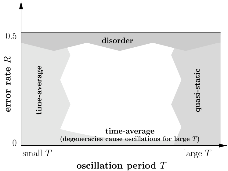
Figure 2: The appearance of a periodic fitness landscape at the border regions of the parameter space.

From the above observations, we can derive generic phase diagrams for periodic fitness landscapes. There are two main possibilities. The fitness landscape may average to a landscape that has a distinct quasispecies, or it may average to a flat landscape. These two cases are illustrated in Fig. 3. Note that the diagrams are meant to illustrate the qualitative form and position of the different phases. In their exact appearance, they may differ substantially from the exact phase diagram of a particular landscape.

If an averaged landscape sports a distinct quasispecies, then for every oscillation period $T$ and every phase of the oscillation $\phi$, we have a unique error threshold $R^{*}(T,\phi)$. For small $T$, the error threshold converges towards that of the average fitness landscape, $R^{*}_{\rm av}$, irrespective of the phase $\phi$. For larger $T$, the error threshold oscillates between $R^{*}_{\rm lo}=\min_{\phi}R^{*}(T,\phi)$ and $R^{*}_{\rm hi}=\max_{\phi}R^{*}(T,\phi)$. In the limit of an infinitely large oscillation period, $R^{*}_{\rm hi}$ converges towards $R^{*}_{\max}$, which is the largest error threshold of all the (static) landscapes ${\mbox{W}}(\phi)$. Similarly, $R^{*}_{\rm lo}$ converges towards $R^{*}_{\min}$ in that limit, where $R^{*}_{\min}$ is accordingly defined as the smallest error threshold of all landscapes ${\mbox{W}}(\phi)$. For a fixed oscillation period $T$ and a fixed error rate $R$ with $R^{*}_{\rm lo}<R<R^{*}_{\rm hi}$ , we have necessarily $R>R^{*}(T,\phi)$ for some phases $\phi$, and $R<R^{*}(T,\phi)$ for the rest of the oscillation period. As a result, a quasispecies will form whenever $R>R^{*}(T,\phi)$, but it will disappear again as soon as $R<R^{*}(T,\phi)$. This phenomenon has for the first time been observed in [17], where the region of the parameter space in which it can be found has been called the temporarily ordered phase. In this phase, whether we observe order or disorder depends on the particular moment in time at which we study the system. Correspondingly, we will call a phase “ordered” only if order can be seen for the whole oscillation period, and we will call a phase “disordered” if during the whole oscillation period no order can be seen. The relationship between the ordered phase, the disordered phase, and the temporarily ordered phase for the first type of landscapes is displayed in Fig. 3a. Compare also the phase diagram of the oscillating Swetina-Schuster landscape in Fig. 4.

In a landscape that averages to a flat one, on the other hand, the disordered phase must extend over the whole range of $R$ for sufficiently small $T$, and order can be observed only above a certain $T_{\min}$. The behavior of the system for small $R$ above $T_{\min}$ cannot in general be predicted solely from the knowledge of Fig. 2. For a landscape with a flat average, the eigenvalues of the monodromy matrix are degenerate for $R=0$. Therefore, in the limit $R\rightarrow 0$, the Perron eigenvector can, in principle, converge to any superposition of the eigenvectors of ${\mbox{X}}(R=0)$. This situation is visualized in Fig. 3b. If the limit corresponds to a non-homogeneous sequence distribution, the ordered phase extends to arbitrarily small $R$ [indicated by the solid line in Fig. 3b]. If, on the other hand, the limit would correspond to a homogeneous sequence distribution, we might find a lower error threshold below which the system would again be in disorder [this is indicated by the dashed line in Fig. 3b]. Since for longer oscillation periods, the oscillations in the degenerate quasispecies at $R=0$ become important, order would be observed for much smaller $R$ with increasing $T$. Hence, the lower disordered phase would fade out for $T\rightarrow\infty$. A study investigating under which situations the ordered phase extends to arbitrarily small $R$ will be presented elsewhere. As a preliminary result, we can state that the limit $R\rightarrow 0$ does in general not lead to a homogeneous sequence distribution.

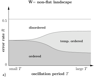
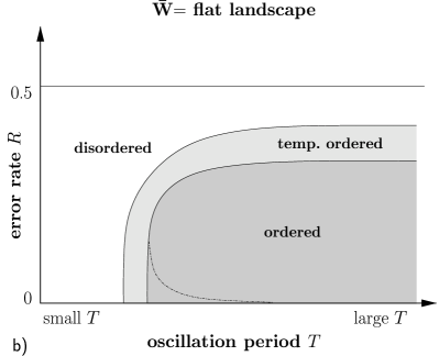
Figure 3: Two possible phase diagrams of a periodic landscape. If ${\mbox{W}}(t)$ averages to a non-flat landscape, there will typically be a lower error threshold, below which we always find order, and a higher error threshold, above which the system is always in a disordered state. If ${\mbox{W}}(t)$ averages to a flat landscape, however, the disordered phase extends to the whole range of $R$ for sufficiently small $T$. The dashed line inside the ordered regime in case b) is explained in the text.

3.2 Discrete approximation

The differential equation formalism we have used so far allows for an elegant discussion of the system’s general properties. However, if we want to obtain numerical solutions, this formalism is not very helpful, because we do not have a general expression for the fundamental matrix ${\mbox{Y}}(t,t_{0})$ from Eq. (40), nor for the monodromy matrix ${\mbox{X}}(t_{0})$ from Eq. (41). Therefore, for a numerical treatment we need to move over to the discretized quasispecies equation,

$$\mbox{\boldmath$y$}(t+\Delta t)=[\Delta t{\mbox{W}}(t)+\mbox{\boldmath$1$}]\mbox{\boldmath$y$}(t)\,.$$ (72)

In the case of constant W, the quasispecies obtained from this equation is identical to that of Eq. (34), and it is also identical to that of equation

$$\mbox{\boldmath$y$}(t+1)={\mbox{W}}\mbox{\boldmath$y$}(t)\,.$$ (73)

Equation (73) has been studied by Demetrius et al. [53], and has been employed by Leuthäusser [49, 10] for her mapping of the quasispecies model onto the Ising model. In the general time-dependent case, however, the additional factor $\Delta t$ and the identity matrix $1$ of Eq. (72) are important, and cannot be left out. The analogue of the fundamental matrix for Eq. (72) reads

$${\mbox{Y}}(t_{0}+k\Delta t,t_{0})={\mathcal{T}}\left\{\prod_{\nu=0}^{k-1}[\Delta t{\mbox{W}}(t_{0}+\nu\Delta t)+\mbox{\boldmath$1$}]\right\}\,,$$ (74)

where ${\mathcal{T}}\{\cdot\}$ indicates that the matrix product has to be evaluated with the proper time ordering [26]. Similarly, the analogue of the monodromy matrix becomes

$${\mbox{X}}(t_{0}) ={\mbox{Y}}(t_{0}+T,t_{0})$$

$$={\mathcal{T}}\left\{\prod_{\nu=0}^{n-1}[\Delta t{\mbox{W}}(t_{0}+\nu\Delta t)+\mbox{\boldmath$1$}]\right\}\,,$$ (75)

where we have assumed that $T$ is an integral multiple of $\Delta t$, and where $n=T/\Delta t$. The influence of the size of $\Delta t$ on the quality of the approximation has been investigated in [26]. A more in-depths discussion of the relationship between the continuous and the discrete quasispecies model can also be found in [19].

3.3 Example landscapes

For the rest of this section, we are going to study several example landscapes, in order to illustrate the implications of our general theory. In all cases considered, we represent the molecules as bitstrings of fixed length $l$. Moreover, we assume that a single bit is copied erroneously with rate $R$, irrespective of the bit’s type and of its position in the string.

3.3.1 One oscillating peak

In previous work on the quasispecies model with periodic fitness landscapes [26, 17], most emphasis has been laid on landscapes with a single oscillating sharp peak. As a generalization of the work of Swetina and Schuster [7], the master sequence has been given a replication rate $A_{0}(t)\gg A$, where $A$ is the replication rate of all other sequences. The replication rate $A_{0}(t)$ has been expressed as

$$A_{0}(t)=A_{0,\rm stat}\exp[\epsilon f(t)]\,,$$ (76)

with a $T$-periodic function $f(t)$. The generic example for that function is $f(t)=\sin(\omega t)$, leading to

$$A_{0}(t)=A_{0,\rm stat}\exp[\epsilon\sin(\omega t)]\,,$$ (77)

The parameter $\epsilon$ allows a smooth crossover from a static landscape to one with considerable dynamics, and the exponential assures that $A_{0}(t)$ is always positive.

In [26, 17] it has been found that the behavior at the border regions of the parameter space is indeed as it is depicted in Fig. 2, and that a phase diagram of the form of Fig. 3a correctly describes the relationship of order and disorder in an oscillating Swetina-Schuster landscape. Here, we put less emphasis on the numerical simulations that lead to these conclusions, but instead show that the phase borders in such a phase diagram can, for an oscillating Swetina-Schuster landscape, be calculated approximately.

For static landscapes with a single peak, the assumption of a vanishing mutational backflow into the master sequence allows to derive an approximate expression for the error threshold [45, 11, 13]. A similar formula can be developed to calculate the error threshold as a function of time in a landscape with a single oscillating peak. But before we turn towards the dynamic landscape, we shall rederive the expression for the master sequence’s concentration $x_{0}$ in a static landscape, based on neglecting mutational backflow. The expression we shall find is slightly more general than the one that was previously given, and it will be of use for the periodic fitness landscape as well.

The 0th component of the quasispecies equation (30) becomes, after neglecting the mutational backflow,

$$\dot{x}_{0}(t)=W_{00}x_{0}(t)-\overline{E}(t)x_{0}(t)\,.$$ (78)

The average excess production $\overline{E}(t)$ can be expressed in terms of $\mbox{\boldmath$x$}(t)$ and W as

$$\overline{E}(t)=\sum_{i,j}W_{ij}x_{j}(t)\,.$$ (79)

With that expression, the solution of Eq. (78) requires the knowledge of the stationary mutant concentrations $x_{j}$, which are usually unknown. To circumvent this problem, we make the somewhat extreme assumption that all mutant concentrations are equal. Although this assumption, which is equivalent to the assumption of equal excess productions $E_{i}$ in the usual calculation without mutational backflow, will generally not be true, it works fine for Swetina-Schuster type landscapes. With this additional assumption, Eq. (79) becomes

$$\overline{E}(t)=\sum_{i}\left[\sum_{j>0}W_{ij}\frac{1-x_{0}(t)}{N-1}+W_{i0}x_{0}(t)\right]\,,$$ (80)

where $N$ is the number of different sequences in the system. When we insert this into Eq. (78) and solve for the steady state, we find

$$x_{0}=\frac{W_{00}-\frac{1}{N-1}\sum_{i}\sum_{j>0}W_{ij}}{\sum_{i}W_{i0}-\frac{1}{N-1}\sum_{i}\sum_{j>0}W_{ij}}\,.$$ (81)

The expressions involving sums over matrix elements in Eq. (81) can be identified with the excess production of the master,

$$E_{0}=\sum_{i}W_{i0}$$ (82)

and with the average excess production without the master,

$$\overline{E}_{-0}=\frac{1}{N-1}\sum_{i}\sum_{j>0}W_{ij}\,,$$ (83)

if W has the standard form ${\mbox{Q}}{\mbox{A}}-{\mbox{D}}$. Therefore, Eq. (81) corresponds to the often quoted result

$$x_{0}=\frac{W_{00}-\overline{E}_{-0}}{E_{0}-\overline{E}_{-0}}\,.$$ (84)

However, Eq. (81) is more general in that it can be used even if W is not given as ${\mbox{Q}}{\mbox{A}}-{\mbox{D}}$.

The idea here is to insert the monodromy matrix into Eq. (81) in order to obtain an approximation for $x_{0}$ in the case of periodic landscapes. But under what circumstances can we expect this to work? After all, Eq. (81) has been derived from an equation with continuous time, Eq. (78), whereas the monodromy matrix advances the system in discrete time steps, as can bee seen in Eq. (43). The important point is here that we are only interested in the asymptotic state, which is given by the normalized Perron vector of the monodromy matrix, whether we use discrete or continuous time. Therefore, we are free to calculate the asymptotic state in a periodic landscape for a given phase $\phi$ from

$$\dot{\mbox{\boldmath$y$}}(t)={\mbox{X}}(\phi)\mbox{\boldmath$y$}(t)\,,$$ (85)

even if this equation does not have a direct physical meaning for finite times. The asymptotic molecular concentrations are then given by the limit $t\rightarrow\infty$ of

$$\mbox{\boldmath$x$}(t)=\frac{\mbox{\boldmath$y$}(t)}{\mbox{\boldmath$e$}\cdot\mbox{\boldmath$y$}(t)}\,.$$ (86)

From differentiating Eq. (86) and inserting Eq. (85), we obtain

$$\dot{\mbox{\boldmath$x$}}(t)={\mbox{X}}(\phi)\mbox{\boldmath$x$}(t)-\mbox{\boldmath$x$}(t)\big{(}\mbox{\boldmath$e$}\cdot[{\mbox{X}}(\phi)\mbox{\boldmath$x$}(t)]\big{)}\,.$$ (87)

When we neglect the backflow onto the master sequence, the 0th component of that equation becomes identical to Eqs. (78) and (79), but with the matrix ${\mbox{X}}(\phi)$ instead of W. This shows that we may indeed use Eq. (81) as an approximation for the asymptotic concentration of $x_{0}$. Of course, since we have neglected mutational backflow, this approximation works only for landscapes in which a single sequence has a significant advantage over all others. But this restriction does equally apply to the static case. Numerically, we have found that Eq. (81) works well for a single oscillating peak, and that it breaks down in other cases as expected.

With the aid of Eq. (81), we are now in the position to calculate the phase diagram of the oscillating Swetina-Schuster landscape. When we insert the monodromy matrix ${\mbox{X}}(\phi)$ into Eq. (81), we are able to obtain (numerically) the error rate at which $x_{0}$ vanishes, $R^{*}(T,\phi)$. From that expression, we can calculate $R^{*}_{\rm lo}$ and $R^{*}_{\rm hi}$. The results of the corresponding, numerically extensive calculations are shown in Fig. 4, together with $R^{*}_{\rm av}$, $R^{*}_{\max}$, and $R^{*}_{\min}$, which have also been determined from Eq. (81).

Figure 4: The phase diagram of an oscillating Swetina-Schuster landscape $[A_{0}(t)=e^{2.4}\exp(2\sin\omega t)]$, obtained numerically from Eq. (81).

We find that both $R^{*}_{\rm lo}$ and $R^{*}_{\rm hi}$ approach $R^{*}_{\rm av}$ for $T\rightarrow 0$, as predicted by our general theory. For $T\rightarrow\infty$, $R^{*}_{\rm hi}$ grows quickly to the level of $R^{*}_{\max}$, but a slight discrepancy between the two values remains. This is due to the complexity of the numerical calculations involved for large $T$. We can only approximate the monodromy matrix by means of Eq. (3.2), and we need ever more factors $\Delta t{\mbox{W}}(t_{0}+\nu\Delta t)+\mbox{\boldmath$1$}$ for large $T$. The discrepancy between $R^{*}_{\rm lo}$ and $R^{*}_{\min}$, on the other hand, has a different origin. The main cause here is the fact that the relaxation into equilibrium is generally slower for smaller error rates. Therefore, $R^{*}_{\rm lo}$ needs a much larger $T$ to reach $R^{*}_{\min}$ than it is the case with $R^{*}_{\rm hi}$ and $R^{*}_{\max}$.

Very recently, Nilsson and Snoad [24] have demonstrated that the method of neglecting back mutations described above can be used to calculate an approximate analytic solution for the oscillating peak. They exploit the fact that if all replication rates except $A_{0}(t)$ are equal to 1, Eq. (78) becomes

$$\dot{x}_{0}(t)=A_{0}(t)x_{0}(t)-\bar{E}(t)x_{0}(t)\,,$$ (88)

with

$$\bar{E}(t)=[A_{0}(t)-1]x_{0}(t)+1$$ (89)

and $Q=(1-R)^{l}$. Eq. (88) can then be solved exactly by introducing a nonlinear transformation

$$x_{0}(t)\rightarrow y(t)=\frac{Q-x_{0}(t)}{[1-Q]x_{0}(t)},$$ (90)

which linearizes the equation. For large $t$, Nilsson and Snoad obtain

$$x_{0}(t)=Q\left[1+(1-Q)\int_{0}^{t}e^{-\int_{s}^{t}[QA_{0}(u)-1]\,du}ds\right]^{-1}\,.$$ (91)

Interestingly, this expression holds for arbitrary $A_{0}(t)$, and not only for periodic ones.

From our discussion in Sec. 3.1, we know that the master sequence’s concentration will, for fast changes, settle to the value corresponding to the average replication rate, and for very slow changes it will be virtually in equilibrium with the current replication rate. In the intermediate regime, we expect the concentration to lag somewhat behind the replication rate. This behavior can be seen as a low-pass filtering of the environmental changes, performed by the evolving population. The idea to look at time-dependent fitness landscapes from that perspective was first introduced by Hirst [27, 28], who reevaluated similar observations made in population genetic models (without explicit landscape) [54, 55, 56, 57]. For the quasispecies model, phase shift and amplitude of the response to a sinusoidal replication rate have been determined computationally in [26], with the result that these curves do indeed have the appropriate form for a low pass filter. Based on Eq. (91), an analytic expression for amplitude and phase shift has been given in [24].

3.3.2 Validity of the expansion in $T$

In the previous section, we have calculated the phase diagram in a landscape with a single oscillating peak. In this section, we are going to asses the validity of the monodromy expansion in $T$ in a similar landscape. Since the integrals involved become very unpleasant if we choose the master sequence’s replication rate to be proportional to $\exp[\sin(\omega t)]$, we study here the related landscape

$$A_{0}(t) =A_{0,\rm stat}[1+\epsilon\sin(\omega t)]\,,$$ (92a)

$$A_{i}(t) =1\quad\mbox{for $i>0$.}$$ (92b)

This landscape follows from expanding Eq. (77) to first order in $\epsilon$. Eq. (50) can be evaluated analytically to arbitrary order for that landscape. In Appendix A, we have carried out the corresponding calculations to 2nd order in $T$.

In Fig. 5, we display the order parameter $m_{s}$ obtained from the expansion of X in terms of $T$ and from the discrete approximation of X as a function of the phase $\phi$ for four different oscillation periods $T$. The results from the two different methods agree well for $T\leq 0.1$, but disagree for larger $T$. The disagreement results from a breakdown of the expansion in $T$ when $T$ becomes large. Note that this breakdown occurs in the vicinity of the radius of convergence that we have estimated in Eq. (63). For the particular landscape of Fig. 5, the estimate guarantees convergence for oscillation periods below approx. 0.1.

Figure 5: Order parameter $m_{s}$ for a landscape with a single oscillating peak, Eq. (92a). The error rate is $R=0.06$. Solid lines stem from the discrete approximation with $n=100$, the dotted lines stem from the expansion in terms of $T$, Eq. (52), evaluated up to second order. Clearly, the expansion Eq. (52) is only of use for relatively short oscillation periods.

3.3.3 Two oscillating peaks

A single oscillating peak provides some initial insights into dynamic fitness landscapes. It is more interesting, however, to study situations in which several sequences obtain the highest replication rate in different phases of the oscillation period. The simplest such case is a landscape in which two sequences in turn become the master sequence. Here, we will assume that the two are located at opposite corners of the boolean hypercube, i.e., that they are given by a sequence and its inverse. In that way, it is possible to group sequences into error classes according to their Hamming distance to one of the two possible master sequences. As an example, we are going to study a landscape with the replication coefficients

$$A_{0}(t) =A_{0,\rm stat}\exp(\epsilon\sin\omega t)\,,$$ (93a)

$$A_{l}(t) =A_{0,\rm stat}\exp(-\epsilon\sin\omega t)\,,$$ (93b)

$$A_{i}(t) =1\quad\mbox{for $0<i<l$.}$$ (93c)

The subscripts in the replication coefficients stand for the Hamming distance to the sequence $000\cdots 0$.

For single peak landscapes, it is instructive to characterize the state of the system at time $t$ by the value of the order parameter $m_{s}(t)$ [Eq. (29)]. In principle, $m_{s}(t)$ can also be used for a landscape with two alternating master sequences if they are each other’s inverse. In that case, the Hamming distance has to be measured with respect to one of the two master sequences. If the population consists only of sequences of the other type of master sequence, we have $m_{s}(t)=-1$. However, there is a small problem with degenerate landscapes in which the two peaks have the same replication rate. In such landscapes, the sequence distribution becomes symmetric with respect to the two peaks, i.e., $x_{0}=x_{l}$, $x_{1}=x_{l-1}$, and so on. Then, $m_{s}(t)$ becomes zero because of this symmetry, although the population may be in an ordered state. To distinguish between the case of true disorder and the case of an ordered, but symmetrical population, we introduce the additional order parameters

$$m_{s}^{+}(t)=\frac{1}{l}\sum_{i=0}^{\lfloor(l-1)/2\rfloor}x_{i}(t)[l-2i]\,,$$ (94)

and

$$m_{s}^{-}(t)=\frac{1}{l}\sum_{i=l-\lfloor(l-1)/2\rfloor}^{l}x_{i}(t)[l-2i]\,.$$ (95)

Here, $\lfloor x\rfloor$ stands for the largest integer smaller than or equal to $x$.

The quantity $m_{s}^{+}(t)$ is always positive, $m_{s}^{-}(t)$ is always negative, and furthermore, we have

$$m_{s}(t)=m_{s}^{+}(t)+m_{s}^{-}(t)\,.$$ (96)

If the population is uniformly distributed over the whole sequence space, we have

$$m_{s}^{+}(t)=-m_{s}^{-}(t)=\frac{1}{l2^{l}}\sum_{i=0}^{\lfloor(l-1)/2\rfloor}\binom{l}{i}(l-2i)\,.$$ (97)

This expression tends to 0 for $l\rightarrow\infty$. If, on the other hand, only the two peaks are populated, each with half of the total population, we find

$$m_{s}^{+}(t)=-m_{s}^{-}(t)=\frac{1}{2}\,.$$ (98)

In the case that either $m_{s}^{+}(t)$ or $m_{s}^{-}(t)$ vanish, the population is centered about the respective other peak.

Figure 6: Order parameters $m_{s}(t)$, $m_{s}^{+}(t)$, $m_{s}^{-}(t)$ as a function of the oscillation phase $\phi=(t\;\mbox{mod}\;T)/T$ in a landscape with two alternating peaks. The upper dashed line represents $m_{s}^{+}(t)$, the lower dashed line represents $m_{s}^{-}(t)$, and the solid line represents $m_{s}(t)$. The sequence length is $l=10$, and we have used $R=0.05$ and $n=T/\Delta t=100$ in all four examples. The parameters of the fitness landscape are $A_{0,\rm stat}=e^{2.4}$, $\epsilon=2$.

In the following, when it is important to distinguish between true disordered populations and symmetric populations, we will use $m_{s}^{+}(t)$ and $m_{s}^{-}(t)$. When the situation is non-ambiguous, we will use $m_{s}(t)$ alone, in order to improve the clarity of our figures.

In Fig. 6, we have displayed $m_{s}^{+}(t)$, $m_{s}^{-}(t)$ and $m_{s}(t)$ for the quasispecies in a fitness landscape of the type defined in Eq. (93). For a large oscillation period, $T=100$, the quasispecies is at every point in time clearly centered around a single peak. The switch from one peak to the other happens very fast. When the landscape oscillates with a higher frequency, the transition time becomes a larger fraction of the total oscillation period. This makes the transition from one peak to the other appear softer in the graphs for smaller oscillation periods. For extremely small oscillations, the system perceives the average fitness landscape, which is a degenerate landscape with two peaks of equal height. As noted above, the quasispecies becomes symmetric in such a landscape. In the lower right of Fig. 6, for $T=0.01$, we can identify this limiting behavior. Both $m_{s}^{+}(t)$ and $m_{s}^{-}(t)$ are nearly constant over the whole oscillation period with an absolute value close to 0.5. The deviation from 0.5 stems from the finite value of the error rate, $R=0.05$ in this example. We observe further that $m_{s}(t)$ lies very close to zero, thus wrongly indicating a disordered state. Note that the absolute value of $m_{s}^{\pm}(t)$ for a uniformly spread population lies, for the parameters of this example, at 0.12 according to Eq. (97).

Observations from the landscape with two oscillating peaks have to be interpreted in the light of results of Schuster and Swetina on static landscapes with two peaks [12], who have found that if the peaks are far away in Hamming distance (which is the case here), a quasispecies is generally unable to occupy both peaks at the same time, unless they are of exactly the same height. For two peaks with different heights, the quasispecies will for small $R$ generally form around the higher peak. For larger $R$, however, the quasispecies moves to the lower peak if it has a higher mutational backflow from mutants, which is the case, for example, if the second peak is broader than the first one. The transition from the higher peak to the lower one with increasing $R$ is very sharp, and can be considered a phase transition. In a dynamic landscape with relatively slow changes, the quasispecies therefore switches the peak quickly when the higher peak becomes the lower one and vice versa.

Figure 7: Order parameter $m_{s}$ as a function of the error rate $R$ for various oscillation phases $\phi=(t\;\mbox{mod}\;T)/T$. The fitness landscape is identical to the one of Fig. 6, and the oscillation period is $T=100$. Note that for $\phi=0.10$, the error threshold seems to have moved towards lower $R$, which is not the case. Instead, the population is symmetric, as would be revealed by graphing $m_{s}^{+}$ or $m_{s}^{-}$.

The exact time at which the switch occurs depends of course on the error rate. The lower the error rate, the longer the population remains centered around the previously higher peak until it actually moves on to the new higher peak. Therefore, if we observe the system at a fixed phase and change the error rate, the quasispecies undergoes, for certain phases $\phi$, a transition similar to the one found in [12] for static landscapes. This is illustrated in Fig. 7, where we display the order parameter $m_{s}$ as a function of the error rate $R$. At the beginning of the oscillation period the quasispecies is, for all error rates $R$ below the error threshold, dominated by the peak corresponding to $m_{s}=-1$. This must be the case, as the replication coefficients of the two peaks intersect at $\phi=0$, so up to this point the quasispecies has not had a chance to build up around the other peak. For phases shortly after $\phi=0$, the quasispecies gains weight around the other peak, starting from the error threshold on downwards. For $\phi=0.15$, we observe a relatively sharp transition from the peak corresponding to $m_{s}=-1$ to the peak corresponding to $m_{s}+1$ at $R\approx 0.05$. The transition then moves quickly towards $R=0$, until the peak corresponding to $m_{s}=1$ dominates the quasispecies for all $R$. For $\phi=0.5$, the replication coefficients intersect again, and the quasispecies is exactly the inverse of the one for $\phi=0$.

4 Aperiodic or stochastic fitness landscapes

As we have seen, periodic fitness landscapes can be treated rather elegantly. We have been able to define a meaningful quasispecies, as well as to determine the general dynamics in the border regions of the parameter space. It would be desirable to obtain similar results for arbitrary dynamic landscapes. After all, an aperiodic or stochastic change is much more realistic than an exactly periodic change. However, the definition of a time-dependent quasispecies is tightly connected to periodic fitness landscapes. For arbitrary changes, the concept of an asymptotic state ceases to be meaningful. Regardless of that, we can derive some results for the border regions of the parameter space. In Section 3.1, we derived the formal solution to Eq. (34),

$$\mbox{\boldmath$y$}(t_{0}+\tau)=\sum_{k=0}^{\infty}\tau^{k}\overline{{\mbox{W}}}_{k}(t_{0},\tau)\mbox{\boldmath$y$}(t_{0})\,.$$ (99)

This can be expanded to first order in $\tau$ as

$$\mbox{\boldmath$y$}(t_{0}+\tau)=\mbox{\boldmath$y$}(t_{0})+\tau\overline{{\mbox{W}}}_{1}(t_{0},\tau)\mbox{\boldmath$y$}(t_{0})\,.$$ (100)

Obviously, the composition of the sequence distribution changes very little over the interval $[t_{0},t_{0}+\tau]$ if the condition

$$\tau\left\|{\overline{{\mbox{W}}}_{1}(t_{0},\tau)}\right\|_{1}\ll 1$$ (101)

is satisfied. This observation allows us to establish a general result for rapidly changing fitness landscapes. If the landscape changes in such a way that for every interval of length $\tau$ beginning at time $t_{0}$, the average

$$\overline{{\mbox{W}}}_{1}(t_{0},\tau)=\frac{1}{\tau}\int_{0}^{\tau}{\mbox{W}}(t_{0}+\tau_{1})d\tau_{1}$$ (102)

is approximately the same for every $t_{0}$, and the condition $\left\|{\smash{\overline{{\mbox{W}}}_{1}(t_{0},\tau)}}\right\|\ll 1/\tau$ holds, then the system develops a quasispecies given by the normalized principal eigenvector of the average matrix $\overline{{\mbox{W}}}_{1}(t_{0},\tau)$. With “approximately the same” we mean that for two times $t_{0}$ and $t_{1}$, the components of the averaged matrices satisfy

$$\left|\Big{(}\overline{{\mbox{W}}}_{1}(t_{0},\tau)\Big{)}_{ij}-\Big{(}\overline{{\mbox{W}}}_{1}(t_{1},\tau)\Big{)}_{ij}\right|<\epsilon\quad\mbox{for all $i$, $j$, $t_{0}$, $t_{1}$,}$$ (103)

with a suitably small $\epsilon$. In other words, if the fitness landscape changes very fast but in stationary way, then the evolving population sees only the time-averaged fitness landscape.

For the special case of $R=0$ we can, as in Eq. (66), write the solution for the quasispecies equation as

$$\mbox{\boldmath$y$}(t)=\exp\left(\int_{t_{0}}^{t}[{\mbox{A}}(t^{\prime})-{\mbox{D}}(t^{\prime})]dt^{\prime}\right)\mbox{\boldmath$y$}(t_{0})\,.$$ (104)

Unlike in the case of a periodic landscape, however, this does not tell us the general behavior at $R=0$, apart from the fact that for fast changes, the system experiences the average fitness landscape. For stochastic landscapes with long time correlations, it is hard to make general statements. The reason for this is that from long time correlations, we cannot generally deduce that the system must be in a quasistatic state. In a landscape that is constant most of the time, but displays intermittent sudden changes, the system can be expected to be mostly in the quasistatic regime. However, one can easily construct landscapes that are in constant flux, and still display long time correlations. Hence, there exists no direct equivalent to the case of periodic fitness landscapes with large oscillation period for general stochastic landscapes. Nevertheless, we can draw a diagram similar to Fig. 2, where for the abscissa, we use the qualitative description “slow” and “fast” changes. Under “fast”, we subsume everything that satisfies the above stated conditions under which the system experiences the average fitness landscape, and under “slow” we subsume everything else, assuming that a parameter exists that allows a smooth transition from the “fast” regime to the “slow” regime. Although Fig. 8 contains considerably less information than Fig. 2, the implications for actual landscapes are more or less the same. Most real landscapes will have a regime that can be associated with slow changes, and hence, we will typically observe phase diagrams of the type of either Fig. 3a) or b).

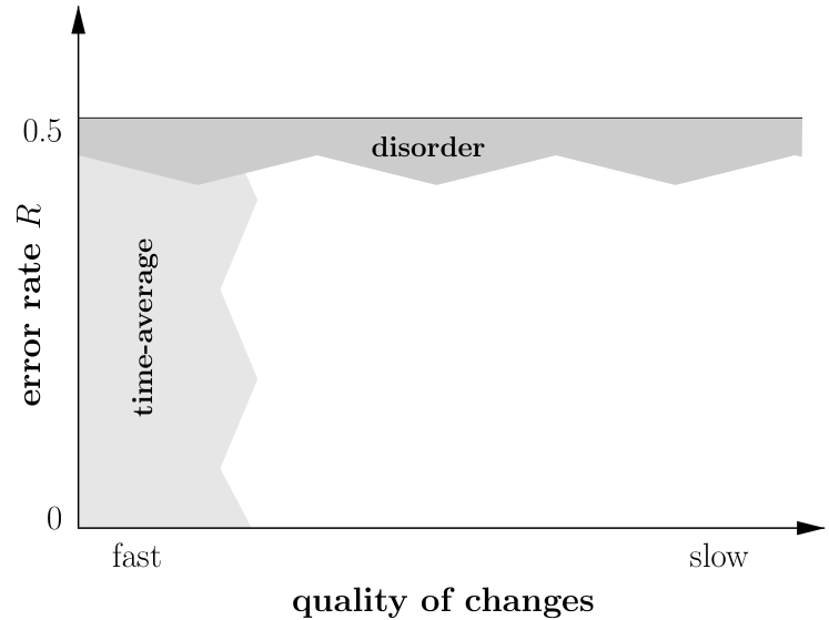
Figure 8: The appearance of a stochastic fitness landscape at the border regions of the parameter space.

As an example, consider the work of Nilsson and Snoad [18], and its subsequent extension by Ronnewinkel et al. [23]. Nilsson and Snoad studied a landscape in which a single peak performs a random walk through sequence space. The peak jumps to a random neighboring position of hamming distance 1 whenever a time interval of length $\tau_{\rm jump}$ has elapsed. Ronnewinkel et al. studied a very similar fitness landscape, but focusing on deterministic movements of the peak that allow for the formal definition of a quasispecies, much as for the case of periodic fitness landscapes in Section 3.1. Ronnewinkel et al. could verify the results of Nilsson and Snoad on more fundamental theoretical grounds.

The parameter $\tau_{\rm jump}$ in the jumping-peak landscape determines whether the changes happen on a short or on a long time scale. If $\tau_{\rm jump}$ is very large, the landscape is static most of the time, and the population has enough time to settle into equilibrium before the peak jumps to a new position. If $\tau_{\rm jump}$ is very small, on the other hand, the peak has moved away long before the population has had the time to form a stable quasispecies. It was found that, for very fast changes, the population fails to track the peak, and selection breaks down. Nilsson and Snoad conclude therefore that “dynamic landscapes have strong constraints on evolvability”. However, this conclusion may have to be reevaluated if we reconsider their landscape from the viewpoint of the general theory developed here. In a fast changing landscape, it is the time-averaged fitness landscape which matters. In the particular example of a randomly moving peak, this average is in general not very meaningful. However, it allows us to render the observations of Nilsson and Snoad plausible, and to understand under what conditions these observations would change. If we consider an interval of length $\tau$ for which Eq. (100) holds, and assume that the changes in the landscape are much faster than $\tau$, i.e., $\tau\ll\tau_{\rm jump}$, then the matrix $\bar{{\mbox{W}}}_{1}(t_{0},\tau)$ will contain a number of peaks with roughly the same (small) selective advantage over the rest of the landscape. In the succeeding interval, the matrix $\bar{{\mbox{W}}}_{1}(t_{0}+\tau,\tau)$ will have a similar structure, but the peaks will be at different positions. In the long run, every single peak position has on average a vanishing selective advantage over every other peak position, and a quasispecies cannot form. However, in the rare case that the peak by chance remains in a small region of the genotype space for a prolonged amount of time, a momentary quasispecies will form there. Thus, in the situation Nilsson and Snoad have studied, selection does not break down due to the mere fact that the landscape is changing fast, but it breaks down because the typical landscape’s average over some time interval yields a highly neutral landscape. If the peak’s movements were such that back jumps would be much more likely, or that the peak would be confined to a small portion of the sequence space, we would clearly see selection. This suggests the viewpoint that the time-averaged landscape determines the “regions of robustness” in the landscape as the regions in which even fast changes in the landscape do not destroy the quasispecies.

In addition to the complete breakdown of adaptation for a fast changing landscape, Nilsson and Snoad observe a sharp decrease of order in their model for very low mutation rates. On first glance, one might be tempted to explain this observation with an asymptotically flat landscape for $R\rightarrow 0$, as described at the end of Sec. 3.1.3. However, this is the wrong explanation in the case of a randomly moving peak. The breakdown of adaptation for small $R$ can be observed for such large $\tau_{\rm jump}$ that for any non-zero $R$, the landscape cannot be considered flat. The true origin of that effect is the population’s convergence onto a single point in the genome space for these low mutation rates. Therefore, the moment the peak position changes, there is no variance in the population that would enable it to move over to the new peak. Note that the nature of this effect is very different from the normal error catastrophe. The error catastrophe occurs because replication is too erroneous to allow for information to be stored in the sequences. As a result, a uniform population forms. In the case of small $R$ in the moving peak landscape, however, the catastrophe occurs because the replication is too faithful. This means in particular that no uniform population forms. Rather, the population always grows to some extent on the new peak position, yet the peak does not rest long enough on that position to allow the sequences to grow to a macroscopic concentration. For the above reasons, we propose to refer to this effect as the convergence catastrophe, as opposed to the error catastrophe, in order to point out that the breakdown of adaptation in that case is not caused by erroneously copied sequences.

Another example of a stochastic fitness landscape is a noisy fitness landscape, i.e., one in which the fitness peaks have a noise term added to them (which means effectively that the population cannot measure the fitness exactly), or one in which a fitness peak has a random position. The first case has been studied by Levitan and Kauffman [58, 59] in the framework of $NK$ landscapes [60, 61], while the second case has been studied in the framework of population genetics by Gillespie [62]. In both cases, it has been observed that the population adapts to the mean fitness, which fits nicely into the general concepts we have presented here.

5 Finite Populations

In the previous sections, we exclusively studied infinite populations. However, as the genotype space generated by even moderately long sequences is exponentially large (there are already $10^{30}$ different sequences of length 100, for example) , it will be essentially empty for any realistic finite population. When most of the possible sequences are not present in the population, the concentration variables become useless, and the outcome of the differential equation formalism may be completely different from the actual behavior of the population. For static fitness landscapes, the effects of a finite population size are reasonably well understood. If the fitness landscape is very simple (a single peak landscape), the population is reasonably well described by finite stochastic sampling from the infinite population concentrations. Moreover, the error threshold generally moves towards smaller $R$ with decreasing population size [14]. In a multi-peak landscape, the finite population localizes relatively quickly around one peak, and remains there, with a dynamics similar to that in a single-peak landscape. In the rare case that a mutant discovers a higher peak, the population moves over to that peak, where it remains again. The main difference between a finite and an infinite population on a landscape with many peaks is given by the fact that the infinite population will always build a quasispecies around the highest peak, whereas the finite population may get stuck on a suboptimal peak. Above the error threshold, a finite population starts to drift through genotype space, irrespective of the landscape.

A finite population on a dynamic landscape will of course show a similar behavior, but in addition to that other effects come into play that are tightly connected to the dynamics of the landscape. The most important difference between static and dynamic landscapes is the possible existence of a temporarily ordered phase in the latter case, which is where we should expect the major new dynamic effects.

In the infinite population limit, the temporarily ordered phase generates an alternating pattern of a fully developed quasispecies and a homogeneous sequence distribution. What changes if a finite population evolves in that phase? At those points in time when a quasispecies is developed, the finite population’s sequence concentrations are given by stochastic sampling from the infinite population result, similarly to static landscapes. As soon as the quasispecies breaks down (and this may happen earlier than the infinite population equations predict, because the error threshold shifts to a lower error rate for a finite population), the population starts to disperse over the landscape. Because of that, the population may loose track of the peak it was centered at previously. Therefore, when the system again enters a time interval in which order should appear, the population may not be able to form a quasispecies, thus effectively staying in the disordered regime, or it may form a quasispecies at a different peak. In this manner, the temporarily ordered phase can create a third possibility for a population to leave a local peak, in addition to the escape via neutral paths or to entropy-barrier crossing, which are present exclusively in static landscapes [63].

5.1 Numerical results

The numerical results presented below have been obtained with a genetic algorithm on $N$ sequences per generation. We have used the following mutation and selection scheme in order to remain as close as possible to the Eigen model:

1. To all sequences $i$ in time step $t$, we assign a probability to be selected and mutated,

   $$p_{i,\rm mut}(t)=\frac{A_{i}(t)}{\sum_{i}[1/\Delta t+A_{i}(t)-D_{i}(t)]n_{i}(t)}\,,$$ (105)

   and a probability to be selected but not mutated,

   $$p_{i,\rm sel}(t)=\frac{1/\Delta t-D_{i}(t)}{\sum_{i}[1/\Delta t+A_{i}(t)-D_{i}(t)]n_{i}(t)}\,.$$ (106)

   Here, $\Delta t$ is the length of one time step, and $n_{i}(t)$ is the number of sequences of type $i$.

2. We choose $N$ sequences at random according to the above defined probabilities $p_{i,\rm mut}(t)$ and $p_{i,\rm sel}(t)\}$. That means, we perform $N$ independent drawings, and in each drawing, a sequence $i$ has a probability $p_{i,\rm sel}(t)\}$ to be copied faithfully into the next generation, and a probability $p_{i,\rm mut}(t)$ to be copied erroneously. The $N$ sequences such generated form the population at time step $t+\Delta t$.

Note that we assume generally

$$D_{i}(t)<\frac{1}{\Delta t}\quad\mbox{for all $i$, $t$,}$$ (107)

so that $p_{i,\rm sel}(t)$ defined in Eq. (106) is always positive.

For an infinite population, such a genetic algorithm evolves according to the equation

$$\mbox{\boldmath$x$}(t+\Delta t)=G\big{(}\mbox{\boldmath$x$}(t),t\big{)}\,,$$ (108)

where $\mbox{\boldmath$x$}(t)$ is the vector of concentrations at time $t$, and $G(\mbox{\boldmath$x$},t)$ is the operator that maps a population at time $t$ onto a population at time $t+1$,

$$G(\mbox{\boldmath$x$},t)=\frac{[\Delta t{\mbox{W}}(t)+\mbox{\boldmath$1$}]\mbox{\boldmath$x$}}{\mbox{\boldmath$e$}^{\rm t}\cdot\big{(}[\Delta t{\mbox{A}}(t)-\Delta t{\mbox{D}}(t)+\mbox{\boldmath$1$}]\mbox{\boldmath$x$}\big{)}}\,.$$ (109)

In Eq. (108), we can replace the non-linear operator $G(\mbox{\boldmath$x$},t)$ with a linear operator $\tilde{G}(\mbox{\boldmath$y$},t)$,

$$\tilde{G}(\mbox{\boldmath$y$},t)=[\Delta t{\mbox{W}}(t)+\mbox{\boldmath$1$}]\mbox{\boldmath$y$}\,.$$ (110)

The linear operator acts on variables $y$ that are related to the concentrations $x$ via

$$\mbox{\boldmath$x$}(t)=\frac{\mbox{\boldmath$y$}(t)}{\mbox{\boldmath$e$}^{\rm t}\cdot\mbox{\boldmath$y$}(t)}\,.$$ (111)

By comparing Eq. (110) with Eq. (72), we observe that there exists a direct correspondence between the genetic algorithm for an infinite population and the discrete quasispecies model. This implies in particular that for periodic landscapes in the genetic algorithm, the expression for the monodromy matrix ${\mbox{X}}(t_{0})$, Eq. (3.2), is exact.

For a finite population, the operator $G(\mbox{\boldmath$x$},t)$ still determines the dynamics. However, the deterministic description Eq. (108) has to be replaced by a probabilistic one, namely Wright-Fisher or multinomial sampling. If $G_{i}(\mbox{\boldmath$x$},t)$ denotes the $i$th component of the concentration vector in the next time step, the probability that a population $\mbox{\boldmath$x$}_{1}=(m_{1},m_{2},\dots)/N,\sum_{i}m_{i}=N$, produces a population $\mbox{\boldmath$x$}_{2}=(n_{1},n_{2},\dots)/N,\sum_{i}n_{i}=N$, in the next time step, is given by

$$P(\mbox{\boldmath$x$}_{1}\rightarrow\mbox{\boldmath$x$}_{2},t)=N!\prod_{i}\frac{G_{i}(\mbox{\boldmath$x$}_{1},t)^{n_{i}}}{n_{i}!}\,.$$ (112)

A proof that the stochastic process described by Eq. (112) does indeed converge to the deterministic process Eq. (108) in the limit $N\rightarrow\infty$ has been given by van Nimwegen et al. [64].

5.1.1 Loss of the master sequence

Figure 9: A single run of a population of $N=1000$ sequences of length $l=15$ in the oscillating Swetina-Schuster landscape. Parameters were $A_{0}(t)=e^{2.4}\exp(2\sin\omega t)$, $A_{i}=1$ for $i>0$, $R=0.06$, $T=100$, $\Delta t=1$. The dashed line indicates the theoretical result for an infinite population.

Our first example of a finite population in a dynamic fitness landscape demonstrates what happens if in the temporarily ordered phase the master sequence is lost due to sampling fluctuations. Fig. 9 depicts a run of a finite population consisting of $N=1000$ sequences of length $l=15$, initialized randomly at $t=0$, in an oscillating Swetina-Schuster landscape. For comparison, we have plotted the theoretical result for an infinite population. The infinite population is always in an ordered state and the order parameter $m_{s}$ never takes on values smaller than 0.2. Nevertheless, the finite population is likely to loose the master sequence whenever the order parameter of the infinite population reaches its minimum, since the error threshold is shifted towards lower error rates for finite populations. In our example run, the master sequence was lost at the end of the first oscillation period, but it was rediscovered shortly afterwards, so that the population could follow the infinite population dynamics for most of the second oscillation period as well. Right after a loss of the master sequence, the probability to rediscover the master has its highest value, because the population is still centered around the master sequence. Once the population has had the time to drift away from the position of the master sequence, the probability of a rediscovery drops rapidly. This is what happened at the end of the second oscillation period. The population completely lost track of the master sequence, and it took the population more than 4 oscillation periods to rediscover it. This is the main difference between a finite and an infinite population in the temporarily ordered phase. For an infinite population, the interval of disorder has the same well-defined length in each oscillation period, whereas for a finite population, once the population has entered the disordered state, it may take a long time until an ordered state is reached again. In fact, for the case of a single peak in a very large sequence space and a small population, the peak may effectively be lost forever once it has disappeared from the population. This can be seen as a dynamic version of Muller’s ratchet [65]. A trait whose advantageous influence on the overall fitness of an individual is reduced at some point (it is not necessary that the trait becomes completely neutral or even deleterious) may be lost from the population due to sampling fluctuations. If at a later stage this trait again becomes very advantageous, it is unavailable to the population until it is rediscovered independently. However, in most cases a rediscovery is very unlikely.

5.1.2 Persistency

Figure 10: A single run of a population of $N=1000$ sequences in a landscape as given in Eq. (93). All parameters were identical to the setup of Fig. 9. The dashed line again indicates the theoretical result for an infinite population.

Another aspect of a finite population in a dynamic landscape is persistency, the tendency of a finite population not to be able to follow the changes in the landscape, even though the infinite population limit predicts this. An example of that effect is shown in Fig. 10. In that example, we have two alternating peaks at opposite corners of the boolean hypercube, as given by Eq. (93). Note that the peaks’ minimal height is relatively small, but still larger than the rest of the landscape’s height. In fact, all parameters are identical to the situation shown in Fig. 9, so that this figure can be seen as an example of the dynamics around one of the peaks in Fig. 10. The infinite population result in Fig. 10 predicts that the population should move to the other peak whenever it becomes the higher one. However, the finite population does not follow this scheme. It stays localized around one of the two peaks for a long time, because a finite population does not occupy all possible points in the sequence space at the same time. Therefore, if a peak grows at a mutational distance far from the currently occupied peak, no sequence in the population is there to exploit the advantage, and hence the new opportunity goes undetected. Only if the population looses track of the first peak, which is possible because of the temporarily ordered phase, it can discover the second peak during its random drift. In the run of Fig. 10, this has happened twice. The first time, the population discovered the alternative peak at the end of the drift, and the second time, it rediscovered this same peak.

Let us compare the case of a finite population in a dynamic landscape with several growing and shrinking peaks to a rugged, but static landscape. In the latter case, once the population has reached a local optimum it remains there, unless a rare mutation opens the possibility to move to a new, higher peak. The same applies to the dynamic situation. But in addition, the fluctuations and oscillations of the fitness values destabilize the population on local optima, and allow it to continue its search for other local optima. If the landscape’s dynamics is such that the population, by following the local optima, moves into regions of low average fitness (observed, e.g., in [26]), the landscape might be called “deceptive”, and in the opposite case, it might be called “well-behaved”.

5.2 A finite population on a simple periodic fitness landscape

5.2.1 The error tail approximation

In the above examples, we saw that the time it takes until the master sequence is rediscovered after it has been lost in the temporarily ordered phase may be much larger than the period length of the landscape. Hence, for several periods, the population does not follow the infinite population results, but remains in a disordered state. It would be desirable to have an analytic description of this behavior, and, in particular, to have an estimate of the probability with which a complete period is skipped, i.e., with which the master sequence is missed for a whole oscillation period. Unfortunately, the continuous time dependency of the master sequence’s replication rate used in Sec. 5.1,

$$A_{0}(t)=A_{0,\rm stat}\exp(\epsilon\sin\omega t)\,,$$ (113)

renders the corresponding calculations very complicated. Instead, we study in this section a simplified fitness landscape that displays a temporarily ordered phase similar to Fig. 9, but that is much easier to handle analytically. For a fitness landscape such as Eq. (113), we can—for sufficiently high error rate $R$—divide the oscillation period into two intervals. During the first interval $I_{1}$, of length $T_{1}$, the population is in an ordered state provided that the master sequence is present in the population, and during the second interval $I_{2}$, of length $T_{2}$, the population is in a disordered state, even if the master sequence is present. The beginning of the first interval need not coincide with the beginning of the oscillation period, but after a suitable shift of the time origin, this is always the case. Note that for a finite population, the second interval is larger than predicted by the infinite population limit, and it may exist even if the infinite population limit predicts a length $T_{2}=0$, because the error threshold is shifted towards smaller error rates for finite populations [14, 66], as discussed previously.

Our approximation here is to keep the fitness landscape constant during the intervals $I_{1}$ and $I_{2}$. During the interval $I_{1}$, we let the master sequence replicate with rate $A_{0}\gg 1$, while all other sequences replicate with $A=1$. During the second interval on the contrary, the fitness landscape becomes flat, i.e., all sequences replicate with $A=1$. We continue to study the discrete process and set $\Delta t=1$, so that $T_{1}$ and $T_{2}$ give the number of time steps spent in each interval. In summary, the replication rate $A_{0}(t)$ satisfies

$$A_{0}(t)=\left\{\begin{array}[]{c@{:\qquad}l}a&\phi\leq T_{1}\\ 1&\mbox{else}\,.\end{array}\right.$$ (114)

In order to obtain expressions that can be treated easily even for a finite population, we use the error tail approximation introduced in [14]. In that approximation, the state of the system is fully described by the concentration of the master sequence. All other sequences are assumed to be uniformly spread over the remaining genotype space. This approximation underestimates the mutational backflow into the master sequence, and hence it underestimates the concentration of the master sequence itself, but this small deviation can be accepted in the light of the enormous simplifications in the calculations.

Before studying the finite population dynamics, let us turn quickly to the infinite population limit. We express the state of the system at time $t$ by a vector $\mbox{\boldmath$x$}(t)=(x_{0}(t),x_{1}(t))^{\rm t}$, where $x_{0}(t)$ is the concentration of the master sequence, while $x_{1}(t)=1-x_{0}(t)$ stands for the total concentration of all other sequences. The generation operator $G(\mbox{\boldmath$x$},t)$ maps the population at time $t$ into the population at time $t+1$, i.e.,

$$\mbox{\boldmath$x$}(t+1)=G\big{(}\mbox{\boldmath$x$}(t),t\big{)}\,.$$ (115)

Here, $G(\mbox{\boldmath$x$},t)$ is given by

$$G(\mbox{\boldmath$x$},t)=\frac{[{\mbox{Q}}{\mbox{A}}(t)+\mbox{\boldmath$1$}]\mbox{\boldmath$x$}}{A_{0}(t)x_{0}+x_{1}+1}\,.$$ (116)

Q is the $2\times 2$ matrix

$${\mbox{Q}}=\left(\begin{array}[]{cc}(1-R)^{l}&\frac{1-(1-R)^{l}}{2^{l}-1}\\ 1-(1-R)^{l}&1-\frac{1-(1-R)^{l}}{2^{l}-1}\end{array}\right)\,,$$ (117)

and ${\mbox{A}}(t)={\rm diag}(A_{0}(t),1)$. The linear operator $\tilde{{\mbox{G}}}(t)={\mbox{Q}}{\mbox{A}}(t)+\mbox{\boldmath$1$}$ describes the evolution of the variables $\mbox{\boldmath$y$}(t)$,

$$\mbox{\boldmath$y$}(t+1)=\tilde{{\mbox{G}}}(t)\mbox{\boldmath$y$}(t)\,,$$ (118)

which map into the original variables via

$$\mbox{\boldmath$x$}(t)=\frac{\mbox{\boldmath$y$}(t)}{\mbox{\boldmath$e$}^{\rm t}\cdot\mbox{\boldmath$y$}(t)}\,,\qquad\mbox{\boldmath$e$}^{\rm t}=(1,1)\,.$$ (119)

Hence, the eigensystem of $\tilde{{\mbox{G}}}$ fully describes the time evolution of $\mbox{\boldmath$x$}(t)$. For the eigenvalues of $\tilde{{\mbox{G}}}$, we find

$$\lambda_{0,1}=\frac{1}{2}\left[\tilde{G}_{00}+\tilde{G}_{11}\pm\sqrt{(\tilde{G}_{00}-\tilde{G}_{11})^{2}+4\tilde{G}_{01}\tilde{G}_{10}}\right]\,,$$ (120)

where the plus sign corresponds to the index 0, and the minus sign corresponds to the index 1. The eigenvectors are

$$\mbox{\boldmath$\phi$}_{0,1} =\frac{1}{1+\xi_{\pm}}\left(1,\xi_{\pm}\right)^{\rm t}\,,$$ (121)

with

$$\xi_{\pm} =\frac{\tilde{G}_{00}-\tilde{G}_{11}}{2\tilde{G}_{01}}\pm\frac{1}{\tilde{G}_{01}}\sqrt{\frac{1}{4}(\tilde{G}_{00}-\tilde{G}_{11})^{2}+\tilde{G}_{01}\tilde{G}_{10}}\,.$$ (122)

Of course, the eigenvalues and the eigenvectors are different for the two intervals $I_{1}$ and $I_{2}$. For the first interval, inserting the explicit expressions for $\tilde{G}_{ij}$ into Eqs. (120)–(122) does not lead to a substantial simplification of the expressions. For the second interval, however, we find for the eigenvalues

$$\lambda^{(2)}_{0} =2\,,$$ (123a)

$$\lambda^{(2)}_{1} =2-\frac{1-(1-R)^{l}}{1-2^{-l}}\,,$$ (123b)

and for the eigenvectors

$$\mbox{\boldmath$\phi$}^{(2)}_{0} =(2^{-l},1-2^{-l})^{\rm t}\,,$$ (124a)

$$\mbox{\boldmath$\phi$}^{(2)}_{1} =(1,-1)^{\rm t}\,.$$ (124b)

The superscript $(2)$ indicates that these results are only valid for the interval $I_{2}$. From the above expressions, we obtain a simple formula for the evolution of the master sequence’s concentration during the interval $I_{2}$ in the following manner. Let the interval start at time $t$, and let the concentration of the master sequence at that moment in time be $x_{0}(t)$. Then we find $n$ time steps later

$$x_{0}(t+n)=\frac{\alpha_{0}\mbox{\boldmath$\phi$}^{(2)}_{0}+\alpha_{1}\left(\lambda^{(2)}_{1}/\lambda^{(2)}_{0}\right)^{n}\mbox{\boldmath$\phi$}^{(2)}_{1}}{\alpha_{0}(\mbox{\boldmath$e$}^{\rm t}\cdot\mbox{\boldmath$\phi$}^{(2)}_{0})+\alpha_{1}\left(\lambda^{(2)}_{1}/\lambda^{(2)}_{0}\right)^{n}(\mbox{\boldmath$e$}^{\rm t}\cdot\mbox{\boldmath$\phi$}^{(2)}_{1})}\,,$$ (125)

where $\alpha_{0}$ and $\alpha_{1}$ have to be chosen such that

$$x_{0}(t)=\alpha_{0}\mbox{\boldmath$\phi$}^{(2)}_{0}+\alpha_{1}\mbox{\boldmath$\phi$}^{(2)}_{1}\,.$$ (126)

After solving Eq. (126) for $\alpha_{0}$ and $\alpha_{1}$ and inserting everything back into Eq. (125), we find

$$x_{0}(t+n)=2^{-l}+\left[x_{0}(t)-2^{-l}\right]\left(1-\frac{1-(1-R)^{l}}{2(1-2^{-l})}\right)^{n}\,.$$ (127)

This formula is sufficiently close to the solution obtained from diagonalization of the full $2^{l}\times 2^{l}$ matrix Q in a flat landscape, and can be considered a good approximation to the actual infinite population dynamics [67]. In principle, a similar formula can be derived for the interval $I_{1}$, but again, the expressions become very complicated and do not lead to any new insight.

Equation (127) demonstrates that a macroscopic proportion of the master sequence that may have built up during the interval $I_{1}$ quickly decays to the expected concentration in a flat landscape, $2^{-l}$.

Let us now study finite population corrections. We assume the duration of the interval $I_{1}$ is long enough so that the quasispecies can form. The asymptotic concentration of the master sequence can then be calculated from a birth and death process as done in [14]. The alternative diffusion approximation used in [66] is of no use here because it allows only replication rates $A_{0}$ of the form $A_{0}=1+\epsilon$ with a small $\epsilon$ [68]. In [14], the probabilities $p_{k}$ to find the master sequence $k$ times in the asymptotic distribution are given by

$$p_{k}=\frac{\tilde{p}_{k}}{\sum_{i=0}^{N}\tilde{p}_{i}}\quad\mbox{with $\tilde{p}_{k}=\frac{\mu^{+}_{k-1}}{\mu^{-}_{k}}\tilde{p}_{k-1}$ and $\tilde{p}_{0}=1$.}$$ (128)

The probabilities $\mu^{+}_{i}$ and $\mu^{-}_{i}$ read here

$$\mu^{+}_{i}=\frac{N-i}{N}\left(\left[\tilde{G}^{(1)}_{00}-1\right]\frac{i}{N}+\tilde{G}^{(1)}_{01}\frac{N-i}{N}\right)$$ (129)

and

$$\mu^{-}_{i}=\frac{i}{N}\left(\tilde{G}^{(1)}_{10}\frac{i}{N}+\left[\tilde{G}^{(1)}_{11}-1\right]\frac{N-i}{N}\right)\,.$$ (130)

The expected asymptotic concentration becomes

$$x_{0}(\infty)=\frac{1}{N}\sum_{k=0}^{N}k\,p_{k}\,.$$ (131)

Unfortunately, there exists no analytic expression for $x_{0}(\infty)$. However, its value is easily computed numerically. With the above assumption about the length of the interval $I_{1}$, we can suppose that at the end of $I_{1}$ the concentration of $x_{0}$ is given by $x_{0}(\infty)$. During the interval $I_{2}$, the concentration of the master sequence will then decay.

5.2.2 The probability to skip one period

If at the end of the interval $I_{2}$ the master sequence has been lost because of sampling fluctuations, and if in addition to that the correlations in the population have decayed so far that we can assume maximum entropy, what is the probability that the master sequence is rediscovered in the following interval $I_{1}$? The process of rediscovering the master consists of two steps. The master sequence has to be generated through mutation, and then it has to be fixated in the population, i.e., it must not be lost again due to sampling fluctuations. First, we calculate the probability $P_{\rm miss}$ that the master is not generated in one time step. This corresponds to the probability that the multinomial sampling of the operator $G^{(1)}(\mbox{\boldmath$x$})$ maps a population $\mbox{\boldmath$x$}=(0,1)^{\rm t}$ into itself. Hence, we have

$$P_{\rm miss} =N!\prod_{i=0}^{1}\frac{G_{i}^{(1)}(\mbox{\boldmath$x$})^{n_{i}}}{n_{i}!}$$

$$=\left(\frac{Q_{11}+1}{2}\right)^{N}=\left[1-\frac{1-(1-R)^{l}}{2^{l+1}-2}\right]^{N}\,.$$ (132)

$G_{i}^{(1)}(\mbox{\boldmath$x$})$ stands for the $i$th component of the outcome of $G^{(1)}(\mbox{\boldmath$x$})$.

The probability that the master sequence becomes fixated requires more work. Denote by $\pi(x,t)$ the probability that the master sequence has reached its asymptotic concentration at time $t$, given that it had the initial concentration $x$ at time $t=0$. The asymptotic concentration is given by $x_{0}(\infty)$ defined in Eq. (131). Then, the probability $\pi(x,t)$ satisfies to second order the backward Fokker-Planck equation

$$\frac{\partial\pi(x,t)}{\partial t}=\langle dx_{0}\rangle\frac{\partial\pi(x,t)}{\partial x}+\frac{\langle(dx_{0})^{2}\rangle}{2}\frac{\partial^{2}\pi(x,t)}{\partial x^{2}}\,.$$ (133)

The moments $\langle dx_{0}\rangle$ and $\langle(dx_{0})^{2}\rangle$ can be calculated along the lines of [64], and we find

$$\langle dx_{0}\rangle =\left(\frac{1}{2}\lambda_{0}^{(1)}-1\right)x_{0}=:\gamma x_{0}\,,$$ (134)

$$\langle(dx_{0})^{2}\rangle =\frac{x_{0}(1-x_{0})}{N}\,.$$ (135)

The solution to Eq. (133) for $t\rightarrow\infty$ is then obtained as in [64], and we find

$$\pi_{\infty} :=\pi\left(\frac{1}{N},\infty\right)=\frac{1-\left(1-\frac{1}{N}\right)^{2N\gamma+1}}{1-\left(1-x_{0}(\infty)\right)^{2N\gamma+1}}$$ (136)

$$\approx 1-e^{-2\gamma}\,.$$ (137)

As the initial concentration of $x_{0}$, we have used $1/N$, since it is—for the parameter settings we are interested in—extremely unlikely that more than one master sequence is generated in one time step. The approximation in the second line is only valid for large population sizes. It generally underestimates the true value of $\pi_{\infty}$.

Note that the expression for $\pi_{\infty}$ given in Eq. (136) reaches the value 1 for the (relatively large) error rate $R$ close to the error threshold for which $x_{0}(\infty)=1/N$. Naively, one would assume that $\pi_{\infty}$ decays with increasing error rate, since mutations increase the risk that good traits are lost, and indeed the approximate expression in Eq. (137) decays with increasing error rate. However, since $\pi_{\infty}$ is the probability that the master sequence reaches its equilibrium concentration, and the equilibrium concentration vanishes close to the error threshold, $\pi_{\infty}$ must rise to 1 at the error threshold.

We have performed simulations with a finite population to test the validity of Eq. (136). For a number of runs, we have initialized the population at random, but with exactly one instance of the master sequence, and have counted how often the master’s concentration reached $x_{0}(\infty)$ and how often it reached 0. The result of these runs are shown in Fig. 11. Clearly, numerical and analytical results are in good agreement.

Finally, we need an estimate of the time $\tau$ it takes from the time the master sequence is discovered to the time in which the equilibrium concentration is reached for the first time. We again follow the calculations in [64], and assume that the process of fixation can be treated in the infinite population limit. From Eq. (116), we obtain for the change in the variable $x_{0}(t)$ during one time step in the interval $I_{1}$

$$x_{0}(t+1)-x_{0}(t)=\frac{-(a-1)x_{0}(t)^{2}+(Q_{00}a-Q_{01}-1)x_{0}(t)+Q_{01}}{(a-1)x_{0}(t)+2}\,.$$ (138)

This can be approximate with a differential equation,

$$\frac{dx_{0}(t)}{dt}\approx x_{0}(t+1)-x_{0}(t)\,,$$ (139)

which we can solve for $t$ as a function of $x_{0}$ to obtain

$$t =\frac{b+4}{z}\left({\rm Atanh}\frac{b-2sx_{0}}{z}-{\rm Atanh}\frac{b-2s/N}{z}\right)$$

$$\qquad\qquad\qquad\qquad\qquad-\frac{1}{2}\ln\frac{-sx_{0}^{2}+bx_{0}+Q_{01}}{-s/N^{2}+b/N+Q_{01}}\,,$$ (140)

with

$$s =a-1\,,$$ (141)

$$b =Q_{00}a-Q_{01}-1\,,$$ (142)

and

$$z=\sqrt{4sQ_{01}+b^{2}}\,.$$ (143)

Therefore, for the estimated time it takes until the master sequence becomes fixated we will use in the following

$$\tau=t\big{(}x_{0}(\infty)\big{)}\,,$$ (144)

with $x_{0}(\infty)$ given in Eq. (131).

We can now calculate the probability that the population skips a whole period, i.e., that it does not find and fixate the master during one interval $I_{1}$. The probability that the master sequence has concentration zero at the beginning of the interval $I_{1}$ is $(1-1/2^{l})^{N}$. Therefore, the probability that the master sequence is not fixated in the first time step is

$$1-\left[1-\left(1-\frac{1}{2^{l}}\right)^{N}\right]\pi_{\infty}\,.$$ (145)

Figure 11: The fixation probability $\pi_{\infty}$ as a function of the error rate $R$ for three different heights of the peak. The solid lines stem from the analytic expression Eq. (136), and the dotted lines stem from measurements on a finite population consisting of $N=500$ sequences.

The probability that the master sequence is not found and subsequently fixated is given by

$$1-(1-P_{\rm miss})\pi_{\infty}\,.$$ (146)

Now, if the master sequence is found, it will roughly take the time $\tau$ given in Eq. (144) until the equilibrium concentration is reached. Therefore, if the master sequence is not found during the first $T_{1}-\tau$ time steps, it normally will not reach the equilibrium concentration in that period. Therefore, in order to calculate the probability $P_{\rm skip}(T_{1})$ that the whole interval $I_{1}$ is skipped, we have to consider only the first $T_{1}-\tau$ time steps of $I_{1}$. In case that $T_{1}<\tau$, we have $P_{\rm skip}(T_{1})\approx 1$. The equality is only approximate, because $\tau$ is the average time until fixation occurs. In rare cases, the fixation may happen much faster.

Of the $T_{1}-\tau$ time steps, the first one is different because during that time step we do not know whether the master sequence is present or not, whereas for the remaining $T_{1}-\tau-1$ time steps we may assume that the master sequence is not present if fixation has not occurred. Therefore, we find

$$P_{\rm skip}(T_{1}) =\left(1-\left[1-\left(1-\frac{1}{2^{l}}\right)^{N}\right]\pi_{\infty}\right)\left[1-\left(1-P_{\rm miss}\right)\pi_{\infty}\right]^{T_{1}-\tau-1}$$ (147)

$$\approx\frac{1-\left[1-\left(1-\frac{1}{2^{l}}\right)^{N}\right]\pi_{\infty}}{1-\left(1-P_{\rm miss}\right)\pi_{\infty}}\exp\left[-(T_{1}-\tau)\left(1-P_{\rm miss}\right)\pi_{\infty}\right]\,.$$ (148)

Figure 12: The probability $P_{\rm skip}(T_{1})$ that the population skips a whole period without fixating the master sequence, as a function of the length of the interval $I_{1}$, for several different settings of $N$ and $R$. The string length is $l=15$.

Figure 12 shows a comparison between this result and numerical simulations. The simulations were carried out by letting a randomly initialized population evolve in a flat landscape for 100 generations, and then recording the time it took the population to find and fixate a peak that was switched on in generation 101. We observe that the analytic expression for $P_{\rm skip}(T_{1})$ predicts the right order of magnitude and the right functional dependency on $T_{1}$, but that it generally underestimates the exact value. Since Eq. (147) contains three quantities for which we have only approximative expressions, namely $P_{\rm miss}$, $\pi_{\infty}$, and $\tau$, at first it is not clear from where these discrepancies arise. However, a systematic check quickly reveals the main cause of the discrepancies. First of all, note that $\tau$ merely shifts the curve to the right. Since the measured and the analytic curves reach the value 1 at very much the same positions in Fig. 12, we can assume that $\tau$, as given by Eq. (144), is accurate enough for our purposes here. Now consider the quantity $\pi_{\infty}$. In Fig. 11, we saw that our expression for $\pi_{\infty}$ generally gives a good estimate of the true value, but that there are some deviations. To check whether these deviations are responsible for the discrepancies visible in Fig. 12, we show additionally $P_{\rm skip}(T_{1})$ with $\pi_{\infty}$ determined numerically. We find that using a numerical $\pi_{\infty}$ enhances the prediction of Eq. (147), in particular for larger error rates. For small error rates, however, the discrepancy is still sizable. Moreover, the analytic expression is generally getting worse for smaller error rates. We can thus conclude that the main problems arise from the expression for $P_{\rm miss}$, Eq. (5.2.2). Indeed, we have derived $P_{\rm miss}$ under a maximum entropy assumption, i.e., we assumed that all mutants are distributed homogeneously over sequence space. Under this assumption, the probability to find the master is exactly the same at every time step. But in reality, the population collapses very rapidly, even in a neutral landscape, and then moves about as a cluster whose radius is determined by the error rate. This introduces very long-range temporal correlations in a population evolving in a flat landscape [69]. In particular, for small error rates the cluster is very small, and this can increase the probability $P_{\rm miss}$ substantially. Note that this effect corresponds to the underestimation of epoch durations that van Nimwegen et al. found in their analysis of the Royal Road genetic algorithm [64]. An exact treatment of this effect would probably have to occur along the lines of [69]. Unfortunately, we cannot simply use their expressions here, because of the term $+\mbox{\boldmath$1$}$ present in our definition of the operator $G(\mbox{\boldmath$x$},t)$ [Eq. (116)].

In order to check the hypothesis that the violation of the maximum entropy condition causes the main discrepancies shown in Fig. 12, we performed additional simulations in which we dispersed the population “by hand” over the complete sequence space in every time step in which the master sequence was not discovered. With this setup, we found a very good agreement between the numerical and the analytical results.

What can we conclude from Eq. (147)? First, note that the true $P_{\rm skip}(T_{1})$ must always be larger than the value predicted by Eq. (147), because the deviations from that value are caused by the population’s collapse into a small cluster. Hence, Eq. (147) is a lower bound on $P_{\rm skip}(T_{1})$, and rediscovery of the peak is less likely than what Eq. (147) predicts. According to our prediction, $P_{\rm skip}(T_{1})$ decays exponentially. This means that the probability to find the peak in one oscillation period,

$$P_{\rm find}(T_{1})=1-P_{\rm skip}(T_{1}),$$ (149)

approaches 1 for large $T_{1}$. This is due to the fact that the peak will certainly be rediscovered if only we wait long enough. However, the model we are studying here is that of a peak that is switched on and off alternatingly, and for which each “on”-period is of fixed length $T_{1}$. In that case, the probability to rediscover the peak within one oscillation period can be extremely small, as we are going to see now. $P_{\rm skip}(T_{1})$ decays with a rate of $(1-P_{\rm miss})\pi_{\infty}$. We can neglect $\pi_{\infty}$ here, as it is of the order of one. Then, the decay rate is for fixed $N$ and large $l$ is approximately given by

$$1-P_{\rm miss}\approx N\frac{1-(1-R)^{l}}{2^{l+1}}\,,$$ (150)

i.e., it decays as $2^{-l}$. This implies in turn that already for string lengths of 50–60 (which can be considered a rough lower bound for typical DNA sequence lengths) and moderate $N$ and $R$, we find $P_{\rm find}(T_{1})\approx 0$ for moderate $T_{1}$. Hence, in many cases it is extremely unlikely that the peak is rediscovered at all.

The above conclusion is of course tightly connected to the fact that we have studied a landscape with a single advantageous sequence. In the other extreme of a wide-peak (Mount Fujiama) landscape, in which the population can sense the peak from every position in the sequence space, the conclusions would be different. Note, however, that neither the single-sharp-peak landscape nor the wide-peak landscape are realistic landscapes. In a realistic, high-dimensional rugged landscape, it is probably valid to assume that local optima, once they are lost from the population, are never rediscovered. In such situations, dynamic fitness landscapes can induce the loss of a local optimum, and thus, they can accelerate Muller’s ratchet[65] like effects.

6 Conclusions

In this report, we have derived several very general results about landscapes with periodic time dependency. First of all, a quasispecies can be defined by means of the monodromy matrix. This means that after a sufficiently long time, the state of the system depends only on the phase $\phi=(t\;\mbox{mod}\;T)/T$ of the oscillation, but not on the absolute time $t$. Therefore, in periodic fitness landscapes, the quasispecies is not a fixed mixture of sequence concentrations. Instead, it is a $T$-periodic function of mixtures of sequence concentrations. We have given an expansion of the monodromy matrix in terms of the oscillation period $T$, which leads to an extremely simple description of the system for very high oscillation frequencies. Namely—if we assume the mutation matrix remains constant at all times—the time-averaged fitness landscape completely determines the behavior of the system, which is essentially indistinguishable from a system in a static landscape. This leads to the important conclusion that selection never ceases to act, no matter how fast the landscape changes. The only exceptions to this rule are due to dynamic landscapes that have a completely flat average. In that case, the system for very fast changes behaves as being subjected to a flat landscape, which is indistinguishable from the behavior of a system above the error threshold. Therefore, if the average landscape is flat, selection will break down if the changes occur with a frequency higher than some critical frequency $\omega^{*}=2\pi/T^{*}$. For very slow changes, on the other hand, the system is virtually in equilibrium all the time. This leads, in general, to a time dependent error threshold $R^{*}(t)$. For mutation rates $R$ such that $\min_{t}R^{*}(t)<R<\max_{t}R^{*}(t)$, the system is below the error threshold for some times $t$, and it is beyond the error threshold for other times. We have dubbed this region of the parameter space the temporarily ordered phase, as we see alternating patterns of order and disorder in that phase (in the infinite population limit). We found these general considerations to be in complete agreement with all example landscapes that we studied.

Periodic fitness landscapes can be fully understood from the knowledge of the monodromy matrix. Therefore, in future work it should be tried to obtain an improved understanding of the properties of that matrix. In particular, an expansion of that matrix in the error rate $R$ would help to further develop the schematic phase diagrams introduced in Sec. 3.1.3.

While the molecular concentrations become $T$-periodic for $t\rightarrow\infty$ in the infinite population limit, this is not necessarily the case when we consider finite populations. In the temporarily ordered phase, after a population has made the transition to the disordered state, it may not transition back to order as the infinite population would. Rather, once the population has lost the ordered state, it is often difficult for the population to return to it. From a very simple analytical model, we found that the probability that the ordered state is not rediscovered in one oscillation period decays exponentially with the length of the interval in which order is possible at all. The decay constant, however, is extremely small for large $l$, and therefore the rediscovery can become very unlikely. In more complex landscapes, this can lead to an acceleration of Muller’s ratchet.

For the case of non-periodic landscapes, we have argued that the main conclusions remain valid, even if our mathematical formalism is not generally applicable in that case. Fast changes in the landscape will average out, whereas slow changes lead to a quasistatic adaption of the quasispecies to the current landscape.

Throughout this report, we have assumed that mutations arise in the copy process. An equally valid assumption is that of mutations arising on a per-unit-time basis (cosmic ray mutations), as opposed to the per generation basis implied by copy mutations. With the latter assumption, one has to study the parallel mutation and selection equations [19] instead of Eigen’s equations. Since these equations can be linearized in the same way as the quasispecies equations, the formalism we developed applies to these equations also. The only difference between the two types of equations is that in the case of cosmic ray mutations, the mutation matrix Q and the replication matrix A are added, whereas in the quasispecies case they are multiplied.

A question that must remain unanswered within the current body of knowledge is to what extent dynamic fitness landscapes help with the progress of evolution. In Sec. 5, we have seen that the dynamics of a fitness landscape can destabilize a population on a local peak. On the one hand, being trapped in a local optimum is regarded as one of the main hindrances to the progress of evolution, so that the destabilizing effect seems to advance evolution. On the other hand, the same effect can lead to the loss of an advantageous trait. Whether the positive or the negative aspect prevails depends most certainly on details of the landscape. In a study of adaptive walks on dynamic $NK$ landscapes, exactly this question was addressed [40]. In that particular case, it was found that for a rapidly changing landscape, the loss of traits was dominant, whereas a slowly changing landscape could lead to a more efficient exploration of the high-fitness regions of genotype space. Apart from this particular study, however, the amount to which a dynamic landscape can advance the progress of evolution is unknown, and deserves more attention in future work.

Appendix A High-frequency expansion of ${\mbox{X}}(t)$ for a single oscillating fitness peak

Eq. (52), gives an expansion of the monodromy matrix for periodic landscapes, ${\mbox{X}}(t_{0})$, in terms of the period length $T$. Here, we calculate the expansion explicitly up to second order for an example landscape. We choose a landscape with a single oscillating peak. The replication rates are

$$A_{0}(t) =a+b\sin(\omega t)\,,$$ (151a)

$$A_{i}(t) =1\qquad\mbox{for all $i>0$}\,.$$ (151b)

In this particular example, we set the decay rates to zero. With vanishing decay rates, the matrix ${\mbox{W}}(t)$ reduces to ${\mbox{Q}}{\mbox{A}}(t)$, and as a consequence, we can write the $n$th average $\overline{{\mbox{W}}}_{k}(t)$ as

$$\left(\overline{{\mbox{W}}}_{k}(t)\right)_{ij}=\sum{\nu_{1}}\sum{\nu_{2}}\cdots\sum{\nu_{k-1}}Q_{i\nu_{1}}Q_{\nu_{1}\nu_{2}}\cdots Q_{\nu_{k-1}j}\overline{A}_{\nu_{1},\nu_{2},\dots\nu_{k-1},j}(t)$$ (152)

with the generalized replication coefficients

$$\overline{A}_{\nu_{1},\dots\nu_{k-1},j}(t)=\frac{1}{T^{k}}\int_{0}^{T}A_{i\nu_{1}}(t_{0}+\tau_{1})\cdots\\ \cdots\int_{0}^{\tau_{k-2}}A_{\nu_{k-1}}(t_{0}+\tau_{k-1})\int_{0}^{\tau_{k-1}}A_{j}(t_{0}+\tau_{k})d\tau_{1}\cdots d\tau_{k}\,.$$ (153)

For the landscape given in Eq. (151), the first order tensor of the generalized replication coefficients has two independent elements, which are (assuming $i>0$)

$$\overline{A}_{0}(t) =a\,,$$ (154a)

$$\overline{A}_{i}(t) =1\,.$$ (154b)

The second order tensor has four independent entries. After some algebra, we obtain (assuming again $i>0$)

$$\overline{A}_{00}(t) =\frac{a^{2}}{2}\,,$$ (155a)

$$\overline{A}_{0i}(t) =\frac{a}{2}-\frac{b}{2\pi}\cos(\omega t)\,,$$ (155b)

$$\overline{A}_{i0}(t) =\frac{a}{2}+\frac{b}{2\pi}\cos(\omega t)\,,$$ (155c)

$$\overline{A}_{ii}(t) =\frac{1}{2}\,.$$ (155d)

In principle, the generalized replication coefficients $\overline{A}_{\nu_{1},\nu_{2},\dots\nu_{k-1},j}(t)$ can be calculated to arbitrary order for the landscape given in Eq. (151). However, the third order tensor has already 8 independent entries, and with every higher order, the number of independent entries doubles.

References

- [1] M. Eigen, Naturwissenschaften 58, 465 (1971).
- [2] C. J. Thompson and J. L. McBride, Math. Biosci. 21, 127 (1974).
- [3] B. L. Jones, R. H. Enns, and S. S. Rangnekar, Bull. Math. Biol. 38, 15 (1976).
- [4] B. L. Jones, Bull. Math. Biol. 41, 761 (1979).
- [5] B. L. Jones, Bull. Math. Biol. 41, 849 (1979).
- [6] M. Eigen and P. Schuster, The Hypercycle—A Principle of Natural Self-Organization (Springer-Verlag, Berlin, 1979).
- [7] J. Swetina and P. Schuster, Biophys. Chem. 16, 329 (1982).
- [8] J. S. McCaskill, J. Chem. Phys. 80, 5194 (1984).
- [9] D. S. Rumschitzki, J. Math. Biol. 24, 667 (1987).
- [10] I. Leuthäusser, J. Stat. Phys. 48, 343 (1987).
- [11] M. Eigen, J. McCaskill, and P. Schuster, J. Phys. Chem. 92, 6881 (1988).
- [12] P. Schuster and J. Swetina, Bull. Math. Biol. 50, 635 (1988).
- [13] M. Eigen, J. McCaskill, and P. Schuster, Adv. Chem. Phys. 75, 149 (1989).
- [14] M. Nowak and P. Schuster, J. theor. Biol. 137, 375 (1989).
- [15] S. Franz and L. Peliti, J. Phys. A 30, 4481 (1997).
- [16] D. Alves and J. F. Fontanari, Phys. Rev. E 57, 7008 (1998).
- [17] C. O. Wilke, C. Ronnewinkel, and T. Martinetz, in Advances in Artificial Life, Proceedings of ECAL’99, Lausanne, Switzerland, Lecture Notes in Artificial Intelligence, edited by D. Floreano, J.-D. Nicoud, and F. Mondada (Springer-Verlag, New York, 1999), pp. 417–421.
- [18] M. Nilsson and N. Snoad, Phys. Rev. Lett. 84, 191 (2000).
- [19] E. Baake and W. Gabriel, Ann. Rev. Comp. Phys. 7, (1999), in press.
- [20] E. Domingo, D. Sabo, T. Taniguchi, and C. Weissmann, Cell 13, 735 (1978).
- [21] C. Adami and C. T. Brown, in Artificial Life IV, edited by R. A. Brooks and P. Maes (MIT Press, Cambridge, MA, 1994), pp. 372–381.
- [22] J. Gomez et al., J. of Viral Hepatitis 6, 3 (1999).
- [23] C. Ronnewinkel, C. O. Wilke, and T. Martinetz, in Theoretical Aspects of Evolutionary Computing, edited by L. Kallel, B. Naudts, and A. Rogers (Springer-Verlag, New York, 2000).
- [24] M. Nilsson and N. Snoad, Quasispecies evolution on a fitness landscape with a fluctuating peak, eprint physics/0004039, April 2000.
- [25] M. Nilsson and N. Snoad, Optimal Mutation Rates in Dynamic Environments, eprint physics/0004042, April 2000.
- [26] C. O. Wilke, Evolutionary Dynamics in Time-Dependent Environments (Shaker Verlag, Aachen, 1999), PhD thesis Ruhr-Universität Bochum.
- [27] T. Hirst, in Fourth European Conference on Artificial Life, edited by P. Husband and I. Harvey (MIT Press, ADDRESS, 1997), pp. 425–431.
- [28] A. J. Hirst and J. E. Rowe, J. theor. Biol. (1998), submitted.
- [29] L. Schmitt, C. L. Nehaniv, and R. H. Fujii, Theor. Comp. Sci. 200, 101 (1998).
- [30] L. Schmitt and C. L. Nehaniv, in Mathematical & Computational Biology: Computational Morphogenesis, Hierarchical Complexity, and Digital Evolution, Lectures on Mathematics in the Life Sciences, edited by C. L. Nehaniv (American Mathematical Society, ADDRESS, 1999), pp. 147–166.
- [31] J. E. Rowe, in Proceedings of GECCO 1999, edited by W. Banzhaf et al. (Morgan Kaufmann, San Mateo, 1999), p. 557.
- [32] J. E. Rowe, in Proceedings of the 2nd Evonet Summerschool (Springer-Verlag, New York, 1999), in press.
- [33] W. Fontana et al., Phys. Rev. E 47, 2083 (1993).
- [34] W. Fontana and P. Schuster, Nature 280, 1451 (1998).
- [35] C. V. Forst, J. Biotechnology 64, 101 (1998).
- [36] C. V. Forst, C. Reidys, and J. Weber, in Advances in Artificial Life, Vol. 929 of Lecture Notes in Artificial Intelligence, edited by F. Morán, A. Moreno, J. J. Merelo, and P. Chacón (Springer, ADDRESS, 1995), pp. 128–147, SFI Preprint 95-10-094.
- [37] M. A. Huynen, P. F. Stadler, and W. Fontana, Proc. Natl. Acad. Sci. USA 93, 397 (1996).
- [38] C. Reidys, P. F. Stadler, and P. Schuster, Bull. Math. Biol. 59, 339 (1997), SFI Preprint 95-07-058.
- [39] E. van Nimwegen, J. P. Crutchfield, and M. Huynen, Proc. Natl. Acad. Sci. USA 96, 9716 (1999).
- [40] C. O. Wilke and T. Martinetz, Phys. Rev. E 60, 2154 (1999).
- [41] N. P. Erugin, Linear System of Ordinary Differential Equations, with Periodic and Quasi-Periodic Coefficients (Academic Press, New York, London, 1966).
- [42] O. Perron, Math. Ann. 64, 248 (1907).
- [43] A. W. M. Dress and D. S. Rumschitzki, Acta Applicandae Mathematicae 11, 103 (1988).
- [44] S. Galluccio, Phys. Rev. E 56, 4526 (1997).
- [45] J. Maynard Smith, Proc. R. Soc. London B 219, 315 (1983).
- [46] P. G. Higgs, Genet. Res. Camb. 63, 63 (1994).
- [47] G. Woodcock and P. G. Higgs, J. theor. Biol. 179, 61 (1996).
- [48] H. Wagner, E. Baake, and T. Gerisch, J. Stat. Phys. 92, 1017 (1998).
- [49] I. Leuthäusser, J. Chem. Phys. 84, 1884 (1985).
- [50] P. Tarazona, Phys. Rev. E 45, 6038 (1992).
- [51] E. Baake, M. Baake, and H. Wagner, Phys. Rev. Lett. 78, 559 (1997).
- [52] Y. A. Yakubovich and V. M. Starzhinskii, Linear Differential Equations with Periodic Coefficients (John Wiley & Sons, New York, 1975), Vol. 1.
- [53] L. Demetrius, P. Schuster, and K. Sigmund, Bull. Math. Biol. 47, 239 (1985).
- [54] A. Sasaki and Y. Iwasa, Genetics 115, 377 (1987).
- [55] K. Ishii, H. Matsuda, Y. Iwasa, and A. Sasaki, Genetics 121, 163 (1989).
- [56] B. Charlesworth, Genet. Res. Camb. 61, 205 (1993).
- [57] R. Lande and S. Shannon, Evolution 50, 434 (1996).
- [58] B. Levitan and S. Kauffman, Molecular Diversity 1, 53 (1995).
- [59] B. Levitan, in Annual Reports in Combinatorial Chemistry and Molecular Diversity, edited by M. R. Pavia, W. H. Moos, A. D. Ellington, and B. K. Kay (ESCOM Publishers, The Netherlands, 1997), Vol. 1, pp. 95–152.
- [60] S. A. Kauffman and S. Levin, J. theor. Biol. 128, 11 (1987).
- [61] S. A. Kauffman, The Origins of Order (Oxford University Press, Oxford, 1992).
- [62] J. H. Gillespie, The Causes of Molecular Evolution (Oxford University Press, Oxford, UK, 1991).
- [63] E. van Nimwegen and J. P. Crutchfield, Metastable Evolutionary Dynamics: Crossing Fitness Barriers or Escaping via Neutral Paths?, eprint adap-org/9907002, 1999.
- [64] E. van Nimwegen, J. P. Crutchfield, and M. Mitchell, Theoretical Computer Science (1997), to appear, SFI working paper 97-04-035.
- [65] H. J. Muller, Mutat. Res. 1, 2 (1964).
- [66] T. Wiehe, E. Baake, and P. Schuster, J. theor. Biol. 177, 1 (1995).
- [67] C. Ronnewinkel, unpublished, 1999.
- [68] W. J. Ewens, Mathematical Population Genetics (Springer-Verlag, New York, 1979).
- [69] B. Derrida and L. Peliti, Bull. Math. Biol. 53, 355 (1991).