Variational Density Matrix Method for Warm Condensed Matter and Application to Dense Hydrogen

Abstract

A new variational principle for optimizing thermal density matrices is introduced. As a first application, the variational many body density matrix is written as a determinant of one body density matrices, which are approximated by Gaussians with the mean, width and amplitude as variational parameters. The method is illustrated for the particle in an external field problem, the hydrogen molecule and dense hydrogen where the molecular, the dissociated and the plasma regime are described. Structural and thermodynamic properties (energy, equation of state and shock Hugoniot) are presented.

I Introduction

Considerable effort has been devoted to systems where finite temperature ions (treated either classically or quantum mechanically by path integral methods) are coupled to degenerate electrons on the Born-Oppenheimer surface. In contrast, the theory for similar systems with non-degenerate electrons ($T$ a significant fraction of $T_{Fermi}$) is relatively underdeveloped except at the extreme high $T$ limit where Thomas-Fermi and similar theories apply. In this paper we present a computational approach for systems with non-degenerate electrons analogous to the methods used for ground state many body computations.

Although an oversimplification, we may usefully view the ground state computations as consisting of three levels of increasing accuracy [1]. At the first level, the ground state wave function consists of determinants, for both spin species, of single particle orbitals often taken from local density functional theory

$$\Psi_{GS}({\bf R})=\left|\begin{array}[]{ccc}\Phi_{1}({\bf r}_{1})&\ldots&\Phi_{N}({\bf r}_{1})\\ \ldots&\ldots&\ldots\\ \Phi_{1}({\bf r}_{N})&\ldots&\Phi_{N}({\bf r}_{N})\\ \end{array}\right|\quad.$$ (1)

The majority of ground state condensed matter calculations stop at this level.

If desired, additional correlations may be included by multiplying the above wave function by a Jastrow factor, $\prod_{i,j}f(r_{ij})$, where the $f$ will also depend on the type of pair (electron-electron, electron-ion). Computing expectations exactly (within statistical uncertainty), with this type of wave function now requires Monte Carlo methods.

Finally diffusion Monte Carlo [2, 3] methods using the nodes of this wave function to avoid the Fermion problem may be used to calculate the exact correlations consistent with the nodal structure.

The finite temperature theory proceeds similarly. Rather than the ground state wave function a thermal density matrix

$$\rho({\bf R},{\bf R^{\prime}};\beta)=\left<{\bf R}|e^{-\beta{\mathcal{H}}}|{\bf R^{\prime}}\right>=\sum_{s}e^{-\beta E_{s}}\Psi_{s}({\bf R})\Psi_{s}({\bf R^{\prime}})$$ (2)

is needed to compute the thermal averages of operators

$$\left<{\bf O}\right>=\frac{\mbox{Tr}\left[{\bf O}\rho\right]}{\mbox{Tr}\left[\rho\right]}\;.$$ (3)

At the first level, this many body density matrix may be approximated by determinants of one-body density matrices, for both spin types, as well as the ions

$$\rho({\bf R},{\bf R^{\prime}};\beta)=\left|\begin{array}[]{ccc}\rho_{1}(r_{1},r^{\prime}_{1};\beta)&\ldots&\rho_{1}(r_{N},r^{\prime}_{1};\beta)\\ \ldots&\ldots&\ldots\\ \rho_{1}(r_{1},r^{\prime}_{N};\beta)&\ldots&\rho_{1}(r_{N},r^{\prime}_{N};\beta)\end{array}\right|$$ (4)

The Jastrow factor can be extended to finite temperature and the above density matrix multiplied by $\prod_{i,j}f(r_{ij},r^{\prime}_{ij};\beta)$. In particular, the high temperature density matrix used in path integral computations has this form.

Finally, the nodal structure from this variational density matrix (VDM) may be used in restricted path integral Monte Carlo (RPIMC) [4, 5, 6, 7, 8]. This method has been extensively applied using the free particle nodes. One aim of the present work is to provide more realistic nodal structures as input to RPIMC.

This paper considers the first level in this approach. The next section is devoted to a general variational principle which will be used to determine the many body density matrix. The principle is then applied to the problem of a single particle in an external potential and compared to exact results for the hydrogen atom density matrix. After a discussion of some general properties, many body applications are considered starting with a hydrogen molecule and then proceeding to warm, dense hydrogen. It is shown that the method and the ansatz considered can describe dense hydrogen in the molecular, the dissociated and the plasma regime. Structural and thermodynamic properties for this system over a range of temperatures (T$=5\,000$ to $250\,000\,K$) and densities (electron sphere radius $r_{s}=1.75$ to $4.0$) are presented.

II Variational Principle for the Many Body Density Matrix

The Gibbs-Delbruck variational principle for the free energy based on a trial density matrix

$$F\leq\mbox{Tr}[\tilde{\rho}{\mathcal{H}}]+kT\;\mbox{Tr}[\tilde{\rho}\ln\tilde{\rho}]$$ (5)

where

$$\tilde{\rho}=\rho/\mbox{Tr}[\rho]$$ (6)

is well known and convenient for discrete systems (e.g. Hubbard models) but the logarithmic entropy term makes it difficult to apply to continuous systems. Here, we propose a simpler variational principle patterned after the Dirac-Frenkel-McLachlan variational principle used in the time dependent quantum problem [9]. Consider the quantity

$$I\left(\frac{\partial\rho}{\partial\beta}\right)=\mbox{Tr}\left(\frac{\partial\rho}{\partial\beta}+{\mathcal{H}}\rho\right)^{2}$$ (7)

as a functional of

$$\Theta\equiv\frac{\partial\rho}{\partial\beta}$$ (8)

$$I\left(\Theta\right)=\mbox{Tr}\left(\Theta+{\mathcal{H}}\rho\right)^{2}$$ (9)

with $\rho$ fixed. $I\left(\Theta\right)=0$ when $\Theta$ satisfies the Bloch equation, $\Theta=-{\mathcal{H}}\rho$, and is otherwise positive. Varying $I$ with $\Theta$ gives the minimum condition

$$\mbox{Tr}\;\left[\delta\Theta\left(\Theta+{\mathcal{H}}\rho\right)\right]=0\quad.$$ (10)

This may be written in a real space basis as

$$\int\int\delta\Theta({\bf R^{\prime}},{\bf R};\beta)\left[\Theta({\bf R},{\bf R^{\prime}};\beta)+{\mathcal{H}}\rho({\bf R},{\bf R^{\prime}};\beta)\right]d{\bf R}d{\bf R^{\prime}}=0$$ (11)

or, using the symmetry of the density matrix in ${\bf R}$ and ${\bf R^{\prime}}$,

$$\int\int\delta\Theta({\bf R},{\bf R^{\prime}};\beta)\left[\Theta({\bf R},{\bf R^{\prime}};\beta)+{\mathcal{H}}\rho({\bf R},{\bf R^{\prime}};\beta)\right]d{\bf R}d{\bf R^{\prime}}=0\quad.$$ (12)

Finally, we may consider a variation at some arbitrary, fixed ${\bf R^{\prime}}$ to get

$$\int\delta\Theta({\bf R},{\bf R^{\prime}};\beta)\left[\Theta({\bf R},{\bf R^{\prime}};\beta)+{\mathcal{H}}\rho({\bf R},{\bf R^{\prime}};\beta)\right]d{\bf R}=0\;\;\forall{\bf R^{\prime}}.$$ (13)

It should be noted that in going from Eq. 11 to Eq. 12 a density matrix symmetric in ${\bf R}$ and ${\bf R^{\prime}}$ is assumed, which is a property of the exact density matrix. If the variational ansatz does not manifestly have this invariance Eq. 13 minimizes the quantity,

$$\int\left[\Theta({\bf R},{\bf R^{\prime}};\beta)+{\mathcal{H}}\rho({\bf R},{\bf R^{\prime}};\beta)\right]^{2}d{\bf R}=0\quad.$$ (14)

We propose solving this equation by parameterizing the density matrix with a set of parameters $q_{i}$ depending on imaginary time $\beta$ and ${\bf R^{\prime}}$,

$$\rho({\bf R},{\bf R^{\prime}};\beta)=\rho({\bf R},q_{1},\ldots,q_{m})\;\;\mbox{where}\;\;q_{i}({\bf R^{\prime}};\beta)$$ (15)

so

$$\Theta({\bf R},{\bf R^{\prime}};\beta)=\sum_{i=1}^{m}\frac{\partial q_{i}({\bf R^{\prime}};\beta)}{\partial\beta}\frac{\partial\rho({\bf R},{q})}{\partial q_{i}}=\sum_{i=1}^{m}\dot{q}_{i}\>\frac{\partial\rho}{\partial q_{i}}\;.$$ (16)

In the imaginary time derivative $\Theta$ only variations in $\dot{q}$ and not ${q}$ are considered since $\rho$ is fixed so,

$$\delta\Theta({\bf R},{\bf R^{\prime}};\beta)=\sum_{i=1}^{m}\delta\dot{q}_{i}({\bf R^{\prime}};\beta)\>\frac{\partial\rho({\bf R},{q})}{\partial q_{i}}\quad.$$ (17)

Using this in equation 13 gives for each variational parameter, since these are independent,

$$\int\!\frac{\partial\rho}{\partial q_{j}}\left(\Theta+{\mathcal{H}}\rho\right)d{\bf R}=0\;\;.$$ (18)

This reveals the imaginary-time equivalent to the approach of Singer and Smith [10] for an approximate solution of the time dependent Schödinger equation using wave packets (see section III). Introducing the notation

$$p_{i}\equiv\frac{\partial(\mbox{ln}\rho)}{\partial q_{i}}$$ (19)

and using Eq. 16, the fundamental set of first order differential equations for the dynamics of the variation parameters in imaginary time follows from Eq.. 18 as,

$$\int\!p_{j}\>\rho{\mathcal{H}}\rho\;d{\bf R}\>\;+\sum_{i=1}^{m}\dot{q}_{i}\int\!p_{j}\>p_{i}\>\rho^{2}\;d{\bf R}\;\;=\;\;0$$ (20)

or in matrix form

$$\frac{1}{2}\frac{\partial H}{\partial\vec{q}}\;+\;\,\stackrel{{\scriptstyle{\textstyle\leftrightarrow}}}{{{\mathcal{N}}}}\>\dot{\vec{q}}=0$$ (21)

where

$$H\equiv\int\rho{\mathcal{H}}\rho\;d{\bf R}$$ (22)

and the norm matrix

$${\mathcal{N}}_{ij}\equiv\int p_{i}\>p_{j}\>\rho^{2}\,d{\bf R}=\lim_{q^{\prime}\rightarrow q}\frac{\partial^{2}N}{\partial q_{i}\partial q^{\prime}_{j}}$$ (23)

with

$$N\equiv\int\rho({\bf R},\vec{q}\,;\beta)\;\rho({\bf R},\vec{q}\>^{\prime}\,;\beta)\;d{\bf R}\;\;.$$ (24)

The initial conditions follow from the free particle limit of the density matrix at high temperature, $\beta\rightarrow 0$,

$$\rho({\bf R},{\bf R^{\prime}};\beta)\rightarrow\exp\left[-({\bf R}-{\bf R^{\prime}})^{2}/4\lambda\beta\right]/(4\pi\lambda\beta)^{3N/2}\quad\mbox{where}\quad\lambda=\hbar^{2}/2m\quad.$$ (25)

Various ansatz forms for $\rho$ may now be used with this approach. After considering the analogy to real time wave packet molecular dynamics, the principle is first applied to the problem of a particle in an external field.

III Analogy to real-time wave packet molecular dynamics

Wave packet molecular dynamics (WPMD) was first used by Heller[11] and later applied to scattering processes in nuclear physics [12] and plasma physics [13, 14]. An ansatz for the wave function $\psi({q_{\nu}})$ is made and the equation of motions for the parameters ${q_{\nu}}$ in real time can be derived from the principle of stationary action [12],

$$\delta\int dt\>L=0\quad,\quad L\left({q_{\nu}}(t),{\dot{q}_{\nu}}(t)\right)=\left\langle\psi\left|i{\partial}_{t}-{\mathcal{H}}\right|\psi\right\rangle$$ (26)

This leads to a set of first order equations, which provides an approximate solution of the Schrödinger equation. However, this principle cannot be directly applied to the Bloch equation because there is no imaginary part in the density matrix. For this reason, we followed in our derivation in section II the principle of Dirac, Frenkel and McLachlan [9], which minimizes the quantity

$$\int|{\mathcal{H}}\psi-i\hbar\theta|^{2}\,dt,\quad\theta=\frac{\partial\psi}{\partial t}\;.$$ (27)

This method was employed in [10] to obtain the dynamical equations in real time.

The VDM approach and WPMD method share the zero temperate limit, which is given by the Rayleigh-Ritz principle (see section V A). At high temperature, the width of wave packets in WPMD grows without limits, which is a known problem of this method [15, 16]. In the VDM approach, the correct high temperature limit of free particles is included. The average width shown in Fig. 10 can be used to verify the attempts to correct the dynamics of the real time wave packets in [16].

IV Example: Particle in an external field

As a first example, we apply this method to the problem of one particle in an external potential

$${\mathcal{H}}=-\lambda{\bf\nabla}^{2}+V(r)\;\;.$$ (28)

The one-particle density matrix will be approximated as a Gaussian with the mean ${\bf m}$, width $w$ and amplitude factor $D$,

$$\rho_{1}({\bf r},{\bf r}^{\prime},\beta)=(\pi w)^{-3/2}\>\mbox{exp}\left\{-\frac{1}{w}({\bf r}-{\bf m})^{2}+D\right\}$$ (29)

as variational parameters. The initial conditions at $\beta\longrightarrow 0$ are $w=4\lambda\beta$, ${\bf m}={\bf r}^{\prime}$ and $D=0$ in order to regain the correct free particle limit, Eq. 25. For this ansatz $H$, defined in Eq. 22 as

$$H\equiv\int\rho{\mathcal{H}}\rho\;d{\bf r}=\left(\frac{3\lambda}{w}+V^{[0]}\right)\frac{e^{2D}}{(2\pi w)^{3/2}}$$ (30)

where

$$V^{[n]}\equiv({2\over\pi w})^{3/2}\int({\bf r}-{\bf m})^{n}V(r)e^{-2({\bf r}-{\bf m})^{2}/w}d{\bf r}$$ (31)

and

$$N\equiv\int\rho\rho^{\prime}d{\bf r}=[\pi(w+w^{\prime})]^{-3/2}\exp\left\{-({\bf m}-{\bf m}^{\prime})^{2}/(w+w^{\prime})\right\}\exp(D+D^{\prime})\quad.$$ (32)

From Eq. 21, the equations for the variational parameters are,

$$\dot{w} = 4\lambda+2wV^{[0]}-\frac{8}{3}V^{[2]}$$ (33)

$$\dot{{\bf m}} = -2{\bf V}^{[1]}$$ (34)

$$\dot{D} = \frac{1}{2}V^{[0]}-\frac{2}{w}V^{[2]}\quad\;.$$ (35)

In absence of a potential, the exact free particle density matrix is recovered. The harmonic oscillator case is also correct since the Gaussian approximation is exact there. For a hydrogen atom, $\lambda=1/2$, $V(r)=-1/r$ and

$$V^{[0]} = -\frac{1}{m}\mbox{erf}\left(m\sqrt{2/w}\right)$$ (36)

$${\bf V}^{[1]} = {{\bf m}\over m^{3}}{w\over 4}\left[\mbox{erf}\left(m\sqrt{2/w}\right)-\sqrt{8\over\pi w}e^{-2m^{2}/w}\right]$$ (37)

$$V^{[2]} = \sqrt{w\over 2\pi}e^{-2m^{2}/w}+{3w\over 4}V^{[0]}\quad.$$ (38)

At low temperature, the density matrix as a function of ${\bf r}$ goes to the ground state wave function as discussed in more detail in the next section. One expects this to be a fixed point of the dynamics of the parameters ${\bf m}$ and $w$ determined by $\dot{{\bf m}}=0$ and $\dot{w}=0$ while $\dot{D}=-E_{0}$. The $\beta\rightarrow\infty$ fixed point: ${\bf m}=0$, $w=9\pi/8$, $\dot{D}=4/3\pi$ (atomic units) corresponds to the well known Rayleigh-Ritz variational result for a Gaussian trial wave function

$$\Psi_{0}({\bf r})=\left(4\over 3\pi\right)^{3/2}\exp(-8r^{2}/9\pi)\;.$$ (39)

In ground state variational studies, addition of two more Gaussians brings the ground state energy to within $0.6$% of exact and similar improvement would be obtained here.

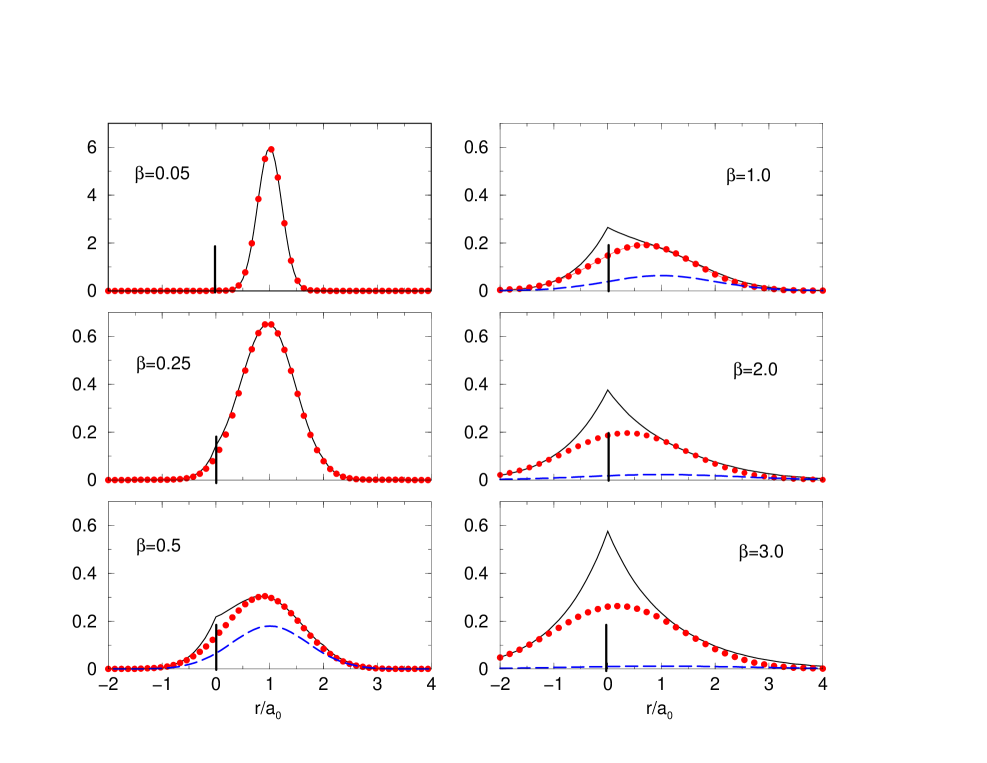
Results at finite $\beta$ require a numerical solution, which is illustrated in the figure below comparing the Gaussian variational density matrix with the exact [17] and the free particle density matrix at several temperatures for the initial condition ${\bf r}^{\prime}=1$. At high temperatures ($\beta=.05$ and $\beta=.25$) the Gaussian approximation correctly reproduces the limiting free particle density matrix. At lower temperatures, the cusp in the exact density matrix due to the Coulombic singularity at the proton becomes evident and the peak shifts to the origin somewhat faster than the Gaussian variational approximation. As $\beta$ increases the exact result grows faster than the variational since the correct energy, -0.5, is lower than $-4/3\pi$ but the Gaussian variational approximation remains rather accurate for $r>1$. The free particle density matrix remains centered at ${\bf r}=1$ and beyond $\beta=0.5$ ($T=54.4$ eV) bears little resemblance to the correct result.

FIG. 1.: Comparison of the Gaussian variational approximation (circles) with the exact density matrix $\rho({\bf r},{\bf r}^{\prime};\beta)$ (solid line) for a hydrogen atom. The free particle density matrix (dashed line) is also shown. The plotted $r$ is along the line from the proton at the origin (marked by the vertical bar) through the initial electron position ${\bf r}^{\prime}=1$.

V Variational Density Matrix Properties

A Zero Temperature Limit

In the preceding section, it was shown that for the hydrogen atom the Gaussian variational density matrix, as a function of ${\bf R}$ converges at low temperature to the Gaussian ground state wave function given by the Rayleigh-Ritz variational principle. It is generally true that the Rayleigh-Ritz ground state corresponds to a $\beta\rightarrow\infty$ of the variational density matrix as we now show.

The Rayleigh-Ritz principle states that for any real parameterized wave function $\Psi({\bf R},q_{1},\ldots,q_{m})$ the variational energy

$$E(\{q\})=\begin{array}[]{c}\underline{\int\psi({\bf R}){\mathcal{H}}\psi({\bf R})\;d{\bf R}}\\ \int\psi({\bf R})^{2}\;d{\bf R}\end{array}$$ (40)

is greater than or equal to the true ground state energy even at the minimum determined by

$$\begin{array}[]{c}\partial\\ \overline{\partial q_{k}}\end{array}E(\{q\})=0\;\;\forall k\;.$$ (41)

For the VDM ansatz, an amplitude parameter $D$ is assumed such that

$$\rho({\bf R},{\bf R^{\prime}};\beta)=e^{D({\bf R^{\prime}};\beta)}\tilde{\rho}({\bf R},\{q({\bf R^{\prime}};\beta)\})\;.$$ (42)

As in the one particle example, it is expected that at low temperature, $\beta\rightarrow\infty$, the other $\dot{q}_{k}\rightarrow 0$ while $\dot{D}\rightarrow$ constant. From this assumption, Eq. 21 implies that as $\beta\rightarrow\infty$

$$\frac{\partial H}{\partial q_{k}}+\dot{D}\frac{\partial N}{\partial q_{k}}=0$$ (43)

for all variational parameters, where we have defined $H\equiv\int\rho{\mathcal{H}}\rho\;d{\bf R}$ and $N\equiv\int\rho^{2}\;d{\bf R}$. Since $\partial H/\partial D=2H$ and $\partial N/\partial D=2N$, Eq. 43 for $q_{k}=D$ implies $\dot{D}=-H/N\equiv-E_{0}$ so Eq. 43 may be rewritten as

$$\frac{\partial}{\partial q_{k}}\left(\frac{H}{N}\right)=0$$ (44)

at the $\beta\rightarrow\infty$ fixed point. With the correspondence

$$\rho({\bf R},\{q({\bf R^{\prime}},\beta)\})\rightarrow e^{D({\bf R^{\prime}};\beta)}\psi({\bf R},\{q\})\quad,$$ (45)

this is equivalent to Eq. 41 and thus the Rayleigh-Ritz ground state corresponds to a zero temperature fixed point in the dynamics of the parameters.

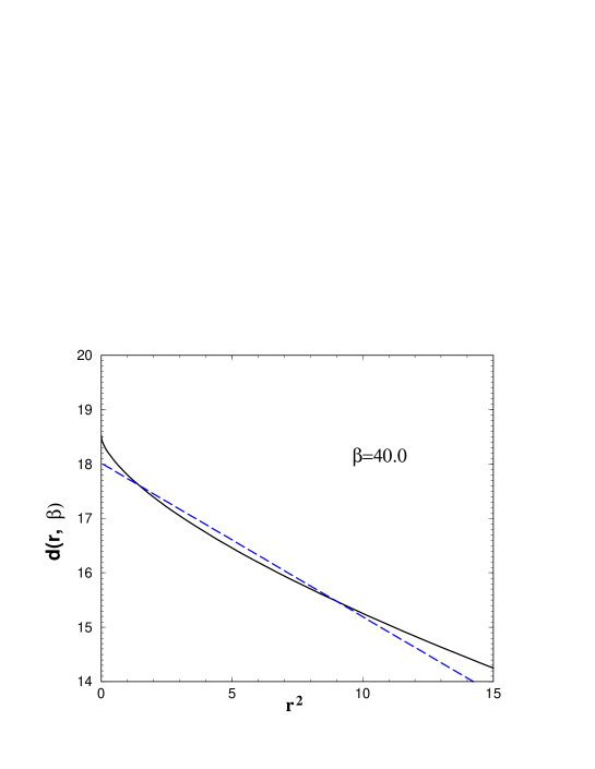
$D$ is a function of ${\bf R^{\prime}}$ and $\beta$, which is calculated by integrating from $\beta=0$ with Eq. 25 as initial conditions. The zero temperature limit of $\dot{D}$ is a constant, $-E_{0}$, which means in the low temperature limit $D$ can written as

$$D({\bf R^{\prime}};\beta)=-\beta E_{0}+f({\bf R^{\prime}})\quad.$$ (46)

The function $f({\bf R^{\prime}})$ can be rewritten as,

$$f({\bf R^{\prime}})=\ln\left\{\psi_{0}({\bf R^{\prime}})\left[\,1+\delta({\bf R^{\prime}})\,\right]\right\}\quad,$$ (47)

where the function $\delta({\bf R^{\prime}})$ is introduced to describe the variational error in the solution of the Bloch equation. It is identical to zero if the variational ansatz includes the exact solution. It leads to loss of symmetry in ${\bf R}$ and ${\bf R^{\prime}}$, which will discussed in the next section. Eq. 45 now reads,

$$\rho({\bf R},{\bf R^{\prime}},\beta\to\infty)=e^{-\beta E_{0}}\psi_{0}({\bf R})\psi_{0}({\bf R^{\prime}})\left[1+\delta({\bf R^{\prime}})\right]$$ (48)

For certain potentials, several fixed points of the dynamics can exist. From Eq. 48, it follows that only the lowest energy state contributes to physical observables calculated from Eq. 3. This completes the argument that the zero temperature limit of the VDM correspond to the Rayleigh-Ritz ground state.

In case of an anti-symmetrized ansatz for the density matrix, one can show that the fixed point of the dynamics in imaginary time corresponds to the Rayleigh-Ritz ground state for an anti-symmetrized wave function.

B Loss of Symmetry

The exact density matrix is symmetric under ${\bf R}\leftrightarrow{\bf R^{\prime}}$. Since we have singled out ${\bf R^{\prime}}$ as the initial point for the imaginary time dynamics, it is not clear that the approximation given in Eq. 29 automatically satisfies this condition. For the free particle limit and the harmonic oscillator, where the Gaussian is the exact solution, it obviously does but in general it does not.

As a specific example, consider again the ground state limit of the hydrogen atom where the Gaussian VDM approximation. Eq. 29 then reads,

$$\lim_{\beta\rightarrow\infty}\;\rho({\bf r},{\bf r}^{\prime};\beta)=e^{D(r^{\prime};\beta)}\;(8/9\pi^{2})^{3/2}e^{-8r^{2}/9\pi}\;.$$ (49)

For this to be symmetric under ${\bf r}\leftrightarrow{\bf r}^{\prime}$, we must have

$$\lim_{\beta\rightarrow\infty}D(r^{\prime};\beta)=-8r^{\prime\,2}/9\pi+c(\beta)$$ (50)

and from the result for $\dot{D}$, $\lim_{\beta\rightarrow\infty}c(\beta)=4\beta/3\pi+c_{1}$.

Figure 2 compares the $D(r,\beta)$ from the Gaussian VDM with Eq. 50 using $c(\beta)=4\beta/3\pi+3/2\ln 2$.

FIG. 2.: $D(r,\beta)$ from the Gaussian approximation in the ground state limit (solid line) of the hydrogen atom. Deviations of this function from linearity indicate a breakdown of symmetry in the Gaussian approximation for $\rho({\bf r},{\bf r}^{\prime};\beta)$. The dashed line is $-8r^{2}/9\pi+4\beta/3\pi+3/2\ln 2$ expected from the Rayleigh-Ritz ground state Eq. 39.

There are several consequences of this small violation of ${\bf R}\leftrightarrow{\bf R^{\prime}}$ symmetry. As shown generally in the section above, in the $\beta\rightarrow\infty$ limit $-\dot{D}$ is the Rayleigh-Ritz variational ground state energy for a Gaussian wave function, which for the hydrogen atom is $E_{0}=-4/3\pi=-0.4244$. Because of the loss of symmetry this is not the same as the energy given by the estimator

$$\left<E\right>=\left<{\mathcal{H}}\right>\equiv\frac{\mbox{Tr}[{\mathcal{H}}\rho]}{\mbox{Tr}[\rho]}$$ (51)

in the $\beta\rightarrow\infty$ limit, which for the hydrogen atom gives the more accurate result $\left<E\right>=-0.4709$. This will be seen again below for the hydrogen molecule where Eq. 51 also gives more accurate ground state energies. Other consequences are less pleasant. Although the energy is more accurate the virial theorem, $\left<K\right>=-\left<U\right>/\,2$, between the kinetic and potential energy is violated by about $3\%$ (while both are more accurate than the usual ground state variational Gaussian result). This has consequences for calculating the equation of state particularly at low density. Slightly more complicated, explicitly symmetric forms for the VDM could be used but in this paper we will continue to explore the basic Gaussian approximation.

C Thermodynamic Estimators

Since the VDM, except in the simplest cases, is not exact various estimators for the same quantity will differ. For example the variational principle introduced in section II consists essentially in globally minimizing the squared difference between $\partial\rho/\partial\beta$ and ${\mathcal{H}}\rho$, either of which can be used in estimating the energy. As mentioned above the energy estimator Eq. 51 and its kinetic and potential energy pieces do not automatically satisfy the virial theorem for Coulomb systems at low density. As an alternative to Eq. 51, one can use the thermodynamic estimators,

$$\left<E\right> = -\left<\frac{\partial}{\partial\beta}\ln\rho\right>,$$ (52)

$$\left<T\right> = -\frac{\lambda}{\beta}\left<\frac{\partial}{\partial\lambda}\ln\rho\right>,$$ (53)

$$\left<V\right> = -\frac{e^{2}}{\beta}\left<\frac{\partial}{\partial e^{2}}\ln\rho\right>$$ (54)

for the total, kinetic and potential energy. These estimators satisfy

$$\left<E\right>=\left<T\right>+\left<V\right>$$ (55)

by the following argument. Any function $f=f(\beta\lambda,\beta e^{2})$ satisfies

$$\beta\frac{\partial f}{\partial\beta}=\lambda\frac{\partial f}{\partial\lambda}+e^{2}\frac{\partial f}{\partial e^{2}}\quad.$$ (56)

From Eq. 21 it follows that all parameters $q_{i}=q_{i}({\bf R^{\prime}};\beta,\lambda,e^{2})$ have this property and therefore so does the variational density matrix.

In the zero temperature limit, the thermodynamic estimators satisfy the virial theorem, which is also satisfied by any exact and any variational Rayleigh-Ritz ground state. From the zero temperature limit of the VDM given by Eq. 48 and the $1/\beta$ factor in Eqs. 53 and 54, it is seen that the symmetry error $\delta({\bf R^{\prime}})$ is unimportant in this limit. It should be noted that calculating the derivatives for $\left<T\right>$ and $\left<V\right>$ increases the numerical work. The pressure is estimated from

$$3\,\left<P\right>v=2\left<K\right>+\left<V\right>\;.$$ (57)

VI Many particle density matrix

We represent the many particle density matrix by a determinant of one-particle density matrices (Eq. 4). It can written as,

$$\rho({\bf R},{\bf R^{\prime}},\beta)=\sum_{\cal{P}}\epsilon_{\cal{P}}\prod_{k}\rho_{1}({\bf r}_{k},{\bf r}^{\prime}_{{\cal{P}}_{k}},\beta)=\sum_{\cal{P}}\epsilon_{\cal{P}}e^{D}\prod_{k}\>(\pi w_{{\cal{P}}_{k}})^{-3/2}\>\mbox{exp}\left\{-\frac{1}{w_{{\cal{P}}_{k}}}({\bf r}_{k}-{\bf m}_{{\cal{P}}_{k}})^{2}\right\}\;.$$ (58)

The permutation sum is over all permutations of identical particles (e.g. same spin electrons) and the permutation signature $\epsilon_{\cal{P}}=\pm 1$. The initial conditions for Eq. 21 are $w_{k}=0$, ${\bf m}_{k}={\bf r}_{k}^{\prime}$, and $D=0$. For this ansatz the generator of the norm matrix, Eq. 24,

$$N=\exp(D+D^{\prime})\,\sum_{\cal{P}}\epsilon_{\cal{P}}\prod_{k}[\pi(w_{k}+w_{{\cal P}_{k}}^{\prime})]^{-3/2}\exp\left\{-({\bf m}_{k}-{\bf m}_{{\cal P}_{k}}^{\prime})^{2}/(w_{k}+w_{{\cal P}_{k}}^{\prime})\right\}\;.$$ (59)

For a periodic system the above equation is also summed over all periodic simulation cell vectors, ${\bf L}$, with ${\bf m}_{k}-{\bf m}_{{\cal P}_{k}}\rightarrow{\bf m}_{k}-{\bf m}_{{\cal P}_{k}}+{\bf L}$. If only the identity permutation is considered the norm matrix is easily inverted so that Eq. 21 gives

$$\dot{w}_{k} = -2w_{k}H_{D}-\frac{8}{3}w_{k}^{2}H_{w_{k}}$$ (60)

$$\dot{{\bf m}}_{k} = -w_{k}H_{{\bf m}_{k}}$$ (61)

$$\dot{D} = -\left(\frac{3}{2}n+1\right)H_{D}-2\sum_{i=1}^{n}w_{i}H_{w_{i}}\quad,$$ (62)

$$\mbox{where}\quad\quad H_{q_{k}} = \frac{1}{2}\frac{\partial H}{\partial q_{k}}\;.$$ (63)

For systems of electrons and ions the full expression for $H_{q_{k}}$ and the norm matrix are derived in Appendix A.

FIG. 3.: Gaussian approximation for the ground state of a hydrogen molecule for bond length $R$. The top left panel shows the Gaussian mean parameter ${\bf m}$ for the two electrons. These stay in the center of the bond (${\bf m}=0$) until about $R=2a_{0}$ and then attach themselves to the separating protons ($\pm\;R/2$). The width parameter, displayed in the lower left panel, makes the transition from the optimal value for a helium atom, $R=0$, to the hydrogen atom result $w=9\pi/8a_{0}^{2}$ at large $R$. The right panel shows the dissociation energy for the singlet state computed from Eq. 51 (open circles with error bars) and the thermodynamic estimator ($-dD/d\beta$) (dashed line) compared to the results of Kolos and Roothan (solid line).

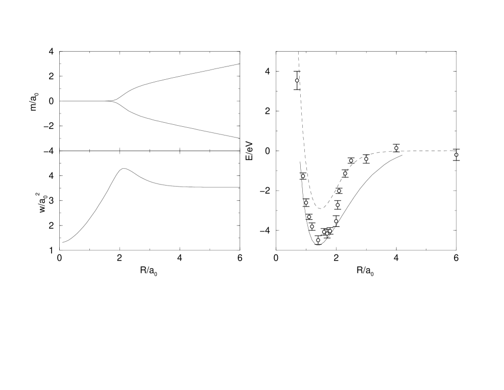
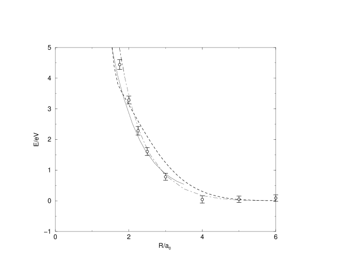
Application to an isolated hydrogen molecule at low temperature is shown in Figure 3. This is for the singlet state (anti-parallel electron spins). The triplet state is considered later after a discussion of how to treat permutation terms in the parameter equations. The bond length at minimum energy is 1.47 a₀, compared with the experimental value of 1.40 a₀. The direct energy estimator Eq. 51 gives a dissociation energy of 4.50 eV at the minimum compared to the experimental value of 4.75 eV. Beyond $R=2$, the energy rises quickly toward the value given by the Rayleigh-Ritz estimator $-dD/d\beta$.

VII Antisymmetry in the Parameter Equations

The determinantal form for the VDM, Eq. 58, is correctly antisymmetric under exchange of identical particles. Since ion exchange effects are negligible at the temperatures considered here these are ignored.

The determinantal form leads to $N!$ terms in the equations of motion for the variational parameters presented in appendix A. It was originally hoped that exchange effects could be ignored in these equations while retaining the full determinantal form for the VDM but this leads to an instability in fermionic systems, e.g. it results in an unphysical strong attraction between two hydrogen molecules.

A practical means of treating all exchange terms, in particular terms involving the potential energy, in the variational parameter equations was not found. Instead it was necessary to use an approximation similar to that used in the real time computations [13, 16]: only pair exchanges in the kinetic energy terms were retained. This will be illustrated for the hydrogen molecule after first giving the explicit form for this correction. It is stressed that, unlike the real time computations, once the variational parameters are determined the full determinantal form is then used in calculating the various averages.

For two particles with parallel spin, the correction term to the kinetic energy is given by,

$$\Delta T = \frac{N_{I}}{N_{AS}}\int\!d{\bf R}\;\rho_{AS}\;\hat{T}\;\rho_{AS}\quad-\quad\int\!d{\bf R}\;\rho_{I}\;\hat{T}\;\rho_{I}$$ (64)

$$\rho_{AS} = \rho_{1}({\bf r}_{1})\rho_{2}({\bf r}_{2})-\rho_{2}({\bf r}_{1})\rho_{1}({\bf r}_{2})\quad,\quad\rho_{I}=\rho_{1}({\bf r}_{1})\rho_{2}({\bf r}_{2})$$ (65)

$$N_{AS} = \int\!d{\bf R}\;\rho_{AS}^{2}\quad,\quad N_{I}=\int\!d{\bf R}\;\rho_{I}^{2}$$ (66)

For the Gaussian ansatz in Eq. 58 it becomes,

$$\Delta T = -\frac{4\lambda N_{I}}{wN_{Q}}\left[\,3\left(1-\tilde{w}^{2}\right)-Q^{2}\right]\quad,$$ (67)

$$w = w_{1}+w_{2}\quad,\quad\tilde{w}=\frac{w}{2\sqrt{w_{1}w_{2}}}\quad,\quad Q^{2}=\frac{2}{w}\left({\bf m}_{1}-{\bf m}_{2}\right)^{2}\quad,\quad N_{Q}=\tilde{w}^{3}e^{Q^{2}}-1\quad.$$ (68)

The corrections to the norm matrix ${\mathcal{N}}$ are neglected in order to keep its analytically invertible form. The corrections to $H_{q_{k}}$ in Eq. 63 are given by

$$\Delta T_{q_{k}}=\frac{1}{2N_{I}}\frac{\partial}{\partial{q_{k}}}\Delta T$$ (69)

The correction to dynamics of the parameters follow from Eq. 60 to 62,

$$\Delta\dot{w}_{1} = -2\,w_{1}\left(\Delta T_{D}+\frac{4}{3}w_{1}\>\Delta T_{w_{1}}\right)$$ (70)

$$\Delta\dot{{\bf m}}_{1} = -w_{1}\>\Delta T_{{\bf m}_{1}}$$ (71)

$$\Delta\dot{D} = -2\left(\Delta T_{D}+w_{1}\>\Delta T_{w_{1}}+w_{2}\>\Delta T_{w_{2}}\right)\quad.$$ (72)

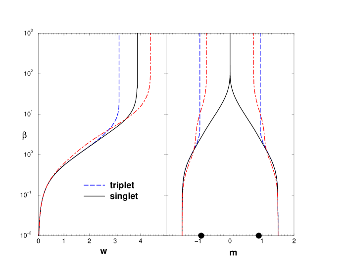
These equations lead to an effective repulsion between the Gaussians for two electrons with parallel spin if there is significant overlap. As a example of this effect the variational parameters for the singlet and triplet states of the hydrogen molecule are compared in Fig. 4. For the triplet state parameters the solution including full exchange effects (long dashed line) are compared with those obtained in the kinetic pair exchange approximation (dot-dashed line). The approximation now prevents the Gaussian means for the same spin electrons from collapsing to the bond center at lower temperature and is numerically close to the solution for full exchange.

FIG. 4.: Effect of antisymmetry on the density matrix parameters, width and mean, for a hydrogen molecule. The protons (large black dots along x axis) are separated by $1.8a_{0}$ and the initial electron positions $r_{e}(\beta=0)=\pm 1.5a_{0}$ along the molecular axis. The solid line for the singlet state (electron spins anti-parallel) shows both electrons centered in the molecular bond at low temperatures (large $\beta$). For the triplet state (parallel electron spins), long dashed line the electrons are centered close to the protons. The approximation of including only kinetic pair exchanges (dot-dashed line) gives a similar result for the mean, with the electrons centered slightly inside the protons but overestimates the Gaussian width (left panel). At high temperature ($\beta\leq 4$) exchange is unimportant and the parameters are nearly the same for all cases.

Even at the lowest temperature considered here in the dense hydrogen simulations ($5000$ K) exchange effects between same spin electrons are negligible beyond a few angstroms, i.e. one or perhaps two nearest neighbors. Fig. 4 for the triplet state thus overestimates the effect likely in dense hydrogen. The main effect of including exchange in the parameter equations is probably to prevent the instability mentioned above.

Fig. 5 shows an energy comparison for the triplet ground state of the hydrogen molecule. First, we compare the Gaussian approximation using only the kinetic exchange term in the parameter equations. For the direct estimator, Eq. 51, one finds fairly good agreement with the quantum chemistry result [18]. The thermodynamic estimator gives a somewhat more repulsive triplet interaction for $R>2a_{0}$. Considering also the Coulomb exchange terms in the Gaussian approximation leads to the dot-dashed line for the thermodynamic estimator. We conclude that leaving out the Coulomb exchange terms in the parameter equations for efficiency reasons is a reasonable approximation in many particle simulations.

FIG. 5.: Energy of repulsion for the triplet ground state of the hydrogen molecule for bond length $R$. The thermodynamic (dashed line) and the direct estimator, Eq. 51, (circles with error bars) for the Gaussian approximation using the kinetic exchange term in the parameter equations are compared with the Kolos and Roothan results (solid line). The thermodynamic estimator for the Gaussian approximation with all exchange terms is shown by the dot-dashed line.

VIII Results from many particle simulations

In this section, we report results from VDM Monte Carlo simulation with 32 pairs of protons and electrons in the temperature and density range of $5\,000\,$K$\,\leq T\leq 250\,000\,$K and $1.75\leq r_{s}\leq 4.0$. Although the Gaussian ansatz VDM will be seen to provide a reasonable model for hydrogen over the full density and temperature regime, a large purpose in presenting these results is to serve as a base for documenting future improvements from better VDMs and the application of RPIMC.

FIG. 6.: Proton-proton pair correlation function from VDM (solid line) and RPIMC (dashed lines at $r_{s}$=1.75, 2.0, and 4.0 for $T\leq 125\,000\,$K).

The proton-proton pair correlation functions are shown in Fig. 6. For temperatures below $20\,000\,$K, a peak emerges near $1.4a_{0}$ that demonstrates clearly the formation of molecules. The comparison with RPIMC simulations [8, 19] at low density shows that the peak positions agree well but RPIMC predicts a significantly bigger height indicating a larger number of molecules. This could be explained by the missing correlations in the VDM ansatz.

At a density of $r_{s}=2.0$, proton-proton pair correlation functions from RPIMC and VDM are almost identical. The area under the peak multiplied by the density gives an estimate for the molecular fraction. By comparing the estimate for different densities one finds that the molecular fraction is diminished when the density is lowered below $r_{s}=2.0$. This effect is well-known and is a result of the increased entropy of dissociated molecules.

Considerable differences between the proton-proton pair correlation functions are found at $r_{s}=1.75$ below $T=20\,000\,K$ where VDM shows still a fair number of molecules while RPIMC predicts a metallic fluid where all bonds are broken as a result of pressure dissociation [8, 20]. This effect has to be verified by RPIMC simulations with VDM nodes because free particle nodes could enhance the transition to a metallic state.

The peak positions shifts from $1.45a_{0}$ at a low density of $r_{s}=4.0$ to $1.3a_{0}$ at $r_{s}=1.75$. The same trend has been found in the RPIMC simulations [8] but the opposite was reported in [21, 22].

FIG. 7.: Proton-electron pair correlation functions from VDM (solid line) and RPIMC (dashed lines at $r_{s}$=1.75, 2.0, and 4.0 for $T\leq 125\,000\,$K).

In the proton-electron pair correlation functions shown in Fig. 7, one finds a strong attraction present even at high temperatures such as $250\,000\,$K. At low temperatures, the electrons are bound in atoms and molecules. This pair correlation function does not show a clear distinction between the two cases. From studying the height of the peak at the origin multiplied by the density, one can estimate the number of bound states at low temperature. Similar to the molecular fraction one finds a reduction of bound electrons with decreasing density below $r_{s}=2.0$. The comparison with PIMC shows that VDM underestimates the height of the peak. This is probably a result of the Gaussian ansatz, which does not satisfy the cusp condition at the proton.

FIG. 8.: Electron-electron pair correlation function for electron with parallel spin from VDM (solid line) and RPIMC (dashed lines at $r_{s}$=1.75, 2.0, and 4.0 for $T\leq 125\,000\,$K).

FIG. 9.: Electron-electron pair correlation function for electron with anti-parallel spin from VDM (solid line) and RPIMC (dashed lines at $r_{s}$=1.75, 2.0, and 4.0 for $T\leq 125\,000\,$K). Note the change in scale in the last row.

Fig. 8 shows the effect of the Pauli exclusion principle leading the a strong repulsion for electrons in the same spin state. This effect is not present in the interaction of electrons with anti-parallel spin (Fig. 9). At high temperature, one observes the effect of the Coulomb repulsion. At low temperature, one finds a peak at the origin that is a result of the formation of molecule, in which two electrons of opposite spin are localized along the bond. The differences to the PIMC graphs can be interpreted as a consequence of different molecular fractions, which has also been observed in Fig. 6.

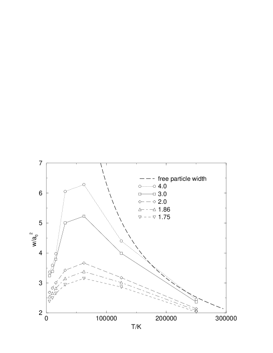
FIG. 10.: Average width of the Gaussian single particle density matrices as a function of temperature for different densities

The average width $w$ of the Gaussian is shown in Fig. 10 as a function temperature and density. At high temperature and low density, one finds only small deviations from the free particle limit. These become more significant with increasing density and decreasing temperature. At low temperature, the attraction to the protons dominates, which leads to a decreasing average width. Finally bound states form and the width approaches a finite limit. At low densities, this is close to the ground state width of the isolated molecule $3.138\,a_{0}^{2}$.

FIG. 11.: Internal energy per atom versus temperature

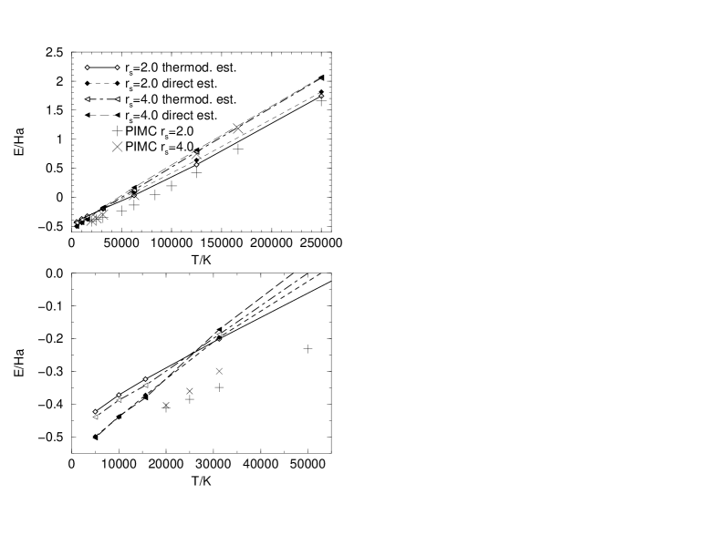
In Fig. 11, we compare the internal energy from the thermodynamic estimator in Eq. 52 and the direct estimator 51. Both agree fairly well at low density. Differences build up with increasing density and decreasing temperature. Comparing with RPIMC simulations, one finds that the VDM energies are generally too high. The magnitude of this discrepancy shows the same dependence on density and temperature like the difference between the two VDM estimators. The difference to the RPIMC results could be explained by the missing correlation effects in the VDM method.

At high temperature, the thermodynamic estimator always gives lower energies than the direct estimator. Below $T=25\,000\,$K, the ordering is reversed. This is consistent with the results from the isolated atom and molecule. The consequence is that the direct estimator is actually closer to the value expected from RPIMC simulations. However, it should be noted that this estimator is not thermodynamically consistent (see section V B).

FIG. 12.: Pressure versus temperature in high and low temperature range. VDM pressure is calculated from virial relation using both the direct and thermodynamic estimators for kinetic and potential energy.

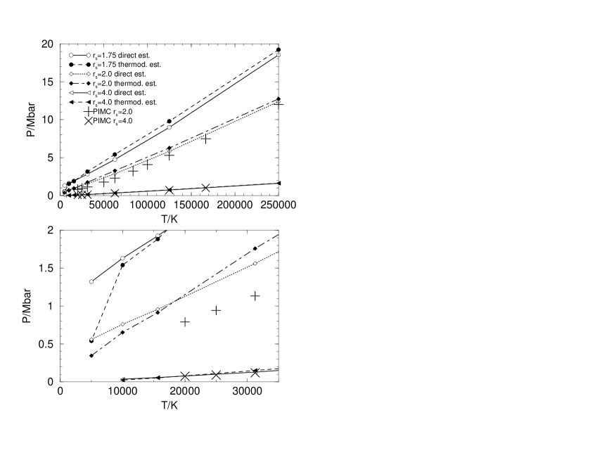
In Fig. 12, we compare pressure as a function of temperature and density from the two VDM estimators with RPIMC results. At low density, the agreement is remarkably good. With increasing density and decreasing temperature, the difference grows. For densities over $r_{s}=2.0$ below $10\,000\,$K, one finds a significant drop in the direct estimator for the pressure. We interpret this effect as a result of the thermodynamic inconsistency.

FIG. 13.: Comparison of experimental and several theoretical Hugoniot functions

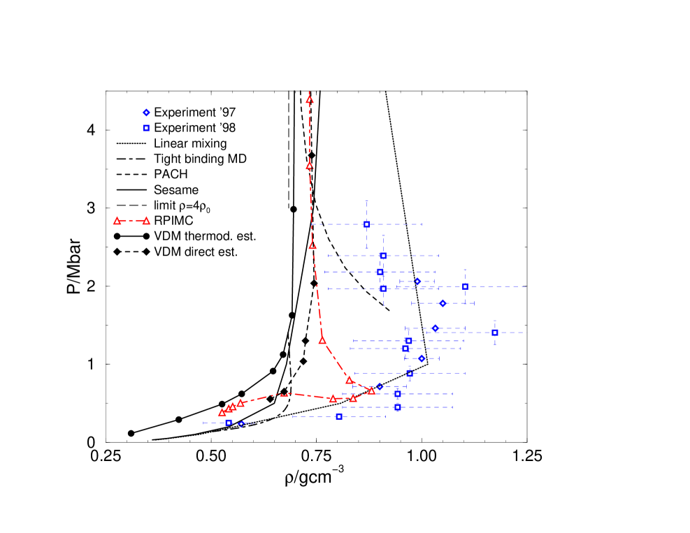
Fig. 13, compares the Hugoniot from Laser shock wave experiments [23, 24] with results from several theoretical approaches (Sesame data base by Kerley [25] (thin solid line), linear mixing model by Ross (dashed line) [26], tight-binding molecular dynamics by Lenosky et.al. [27] (dash-dotted line), Padé approximation in the chemical picture by Ebeling et.al. [28] (dotted line), RPIMC simulations [29] (triangles), VDM direct estimator (full diamonds) and VDM thermodynamic estimator (full circles)). The long dashed line indicates the theoretical high pressure limit $\rho=4\rho_{0}$ of the fully dissociated non-interacting plasma. In the experiments, a shock wave propagates through a sample of precompressed liquid deuterium characterized by its initial state, ($E_{0}$, $V_{0}$, $p_{0}$). Assuming an ideal shock front, the variables of the shocked material ($E$, $V$, $p$) satisfy the Hugoniot relation [30],

$$H=E-E_{0}+\frac{1}{2}(V-V_{0})(p+p_{0})=0\quad.$$ (73)

The initial conditions in the experiment were $T=19.6\,\rm{K}$ and $\rho=0.171\,\rm{g/cm^{3}}$. We set $V_{0}=39.1\,\rm{\AA^{3}}$ and $p_{0}\approx 0$. We show two VDM curves based on the thermodynamic and direct estimators. For $E_{0}$, we use the corresponding value of the ground state of the isolated hydrogen molecule, $E_{0}^{th}=-0.955\,\rm{Ha}$ and $E_{0}^{dir}=-1.124\,\rm{Ha}$.

We expect the difference of the two estimators to give a rough estimate of the accuracy of the VDM approach. At high temperature, the difference is relatively small and agreement with RPIMC simulations is reasonable. Both VDM estimators indicate that there is maximal compressibility around 1.5 Mbar. However, in this regime of high density and relatively low temperature a more careful study seems unavoidable. We suggest RPIMC simulations using the VDM nodal surface to restrict the paths.

IX Conclusions

The VDM approach provides a way to systematically improve the many particle density matrix. Already the simplest ansatz using one Gaussian to describe the single particle density matrices gives a good description of hydrogen in the discussed range of temperature and density. The method includes the correct high temperature behavior and shows the expected formation of atoms and molecules. The thermodynamic variables are in reasonable agreement with RPIMC simulations. The presented Gaussian ansatz can be improved in several ways. One could use a sum of Gaussians, add underestimated correlation effects by including a Jastrow factor in the ansatz or use a two-step path integral. Further one can use this essentially analytic density matrix to furnish the nodal surface in RPIMC simulations, replacing the free particle nodes by a density matrix that already includes the principle physical effects. This level of accuracy seems to be required to determine a Hugoniot function that is very sensitive to the different level of approximations made by various theories.

A Gaussian Approximation Interaction Terms

The general equations for the variational parameters ${q}$ in a parameterized density matrix, from Eq. 21, are

$$\frac{1}{2}\frac{\partial H}{\partial\vec{q}}\;+\;\,\stackrel{{\scriptstyle{\textstyle\leftrightarrow}}}{{{\mathcal{N}}}}\>\dot{\vec{q}}=0$$ (A1)

where

$$H\equiv\int\rho{\mathcal{H}}\rho\;d{\bf R}=\int\rho{\mathcal{H}}\rho_{I}d{\bf R}$$ (A2)

and the norm matrix

$${\mathcal{N}}_{ji}\equiv\int p_{j}\>p_{i}\>\rho^{2}\,d{\bf R}=\lim_{q^{\prime}\rightarrow q}\frac{\partial^{2}N}{\partial q_{j}\partial q^{\prime}_{i}}$$ (A3)

with

$$N\equiv\int\rho({\bf R},\vec{q}\,;\beta)\;\rho({\bf R},\vec{q}\>^{\prime}\,;\beta)\;d{\bf R}\;\;.$$ (A4)

The subscript $I$ in Eq. A2 indicates that only one $\rho$ needs to be antisymmetric and the identity permutation can be used in the other. (We are also dropping $1/N!$ prefactors which are the same for the norm matrix and thus cancel out.) This appendix contains the detailed formulae for these equations for a parameterized Gaussian density matrix applied to a Coulomb system.

Repeating Eq. 58 the parameterized variational density matrix is an anti-symmetrized product of one-particle density matrices,

$$\rho({\bf R},{\bf R^{\prime}},\beta)=\sum_{\cal{P}}\epsilon_{\cal{P}}\prod_{k}\rho_{1}({\bf r}_{k},{\bf r}^{\prime}_{{\cal{P}}_{k}},\beta)=\sum_{\cal{P}}\epsilon_{\cal{P}}e^{D}\prod_{k}\>(\pi w_{{\cal{P}}_{k}})^{-3/2}\>\mbox{exp}\left\{-\frac{1}{w_{{\cal{P}}_{k}}}({\bf r}_{k}-{\bf m}_{{\cal{P}}_{k}})^{2}\right\}$$ (A5)

where the amplitude $D$ and the widths $w_{k}$ and means ${\bf m}_{k}$ are the variational parameters. The permutation sum is over all permutations of identical particles (e.g. same spin electrons) and $\epsilon_{\cal{P}}=\pm 1$is the permutation signature. The initial conditions are $w_{k}=0$, ${\bf m}_{k}={\bf r}_{k}^{\prime}$, and $D=0$.

For this ansatz the generator of the norm matrix,

$$N=\sum_{\cal{P}}\epsilon_{\cal{P}}\prod_{k}[\pi(w_{k}+w_{{\cal P}_{k}}^{\prime})]^{-3/2}\exp\left\{-({\bf m}_{k}-{\bf m}_{{\cal P}_{k}}^{\prime})^{2}/(w_{k}+w_{{\cal P}_{k}}^{\prime})\right\}\exp(D+D^{\prime})\;.$$ (A6)

For a periodic system the above equation also is summed over all periodic simulation cell vectors, ${\bf L}$, with ${\bf m}_{k}-{\bf m}_{{\cal P}_{k}}^{\prime}\rightarrow{\bf m}_{k}-{\bf m}_{{\cal P}_{k}}^{\prime}+{\bf L}$. Using this the components of the norm matrix are then:

$${\mathcal{N}}_{DD} = \sum_{\cal{P}}\epsilon_{\cal{P}}N_{\cal P}$$ (A7)

$${\mathcal{N}}_{{\bf m}_{i}D} = \sum_{\cal P}\epsilon_{\cal P}\left[{-2({\bf m}_{i}-{\bf m}_{{\cal P}_{i}})\over w_{i}+w_{{\cal P}_{i}}}\right]N_{{\cal P}}$$ (A8)

$${\mathcal{N}}_{w_{i}D} = \sum_{\cal P}\epsilon_{\cal P}\left({-1\over w_{i}+w_{{\cal P}_{i}}}\right)\left[{3\over 2}-{({\bf m}_{i}-{\bf m}_{{\cal P}_{i}})^{2}\over w_{i}+w_{{\cal P}_{i}}}\right]N_{\cal P}$$ (A9)

$${\mathcal{N}}_{{\bf m}_{i}{\bf m}_{j}} = \sum_{\cal P}\epsilon_{\cal P}\left[{2\delta_{j,{\cal P}_{i}}\stackrel{{\scriptstyle{\textstyle\leftrightarrow}}}{{I}}\over w_{i}+w_{j}}+4{({\bf m}_{i}-{\bf m}_{{\cal P}_{i}})\over(w_{i}+w_{{\cal P}_{i}})}{({\bf m}_{j}-{\bf m}_{{\cal P}_{j}^{-1}})\over(w_{j}+w_{{\cal P}_{j}^{-1}})}\right]N_{\cal P}$$ (A10)

$${\mathcal{N}}_{{\bf m}_{i}w_{j}} = \sum_{\cal{P}}\epsilon_{\cal{P}}\left[{\delta_{j,{\cal P}_{i}}\over w_{i}+w_{j}}+{1\over(w_{j}+w_{{\cal P}_{j}^{-1}})}\left({3\over 2}-{({\bf m}_{j}-{\bf m}_{{\cal P}_{j}^{-1}})^{2}\over(w_{j}+w_{{\cal P}_{j}^{-1}})}\right)\right]\left[{2({\bf m}_{i}-{\bf m}_{{\cal P}_{i}})\over w_{i}+w_{{\cal P}_{i}}}\right]N_{\cal P}$$ (A11)

$${\mathcal{N}}_{w_{i}w_{j}} = \sum_{\cal{P}}\epsilon_{\cal{P}}\left\{{\delta_{j,{\cal P}_{i}}\over(w_{i}+w_{{\cal P}_{i}})^{2}}\left[{3\over 2}-{2({\bf m}_{i}-{\bf m}_{{\cal P}_{i}})^{2}\over w_{j}+w_{{\cal P}_{j}}}\right]\right.+{1\over(w_{i}+w_{{\cal P}_{i}})(w_{j}+w_{{\cal P}_{j}^{-1}})}$$ (A13)

$$\hskip 36.135pt\left.\left[{3\over 2}-{({\bf m}_{i}-{\bf m}_{{\cal P}_{i}})^{2}\over w_{i}+w_{{\cal P}_{i}}}\right]\left[{3\over 2}-{({\bf m}_{j}-{\bf m}_{{\cal P}_{j}^{-1}})^{2}\over w_{j}+w_{{\cal P}_{j}^{-1}}}\right]\right\}N_{\cal P}$$

where (A14)

$$N_{\cal P} = e^{2D}\prod_{j}\begin{array}[]{c}\underline{\exp\left\{-\frac{({\bf m}_{j}-{\bf m}_{{\cal P}_{j}})^{2}}{(w_{j}+w_{{\cal P}_{j}})}\right\}}\\ (\pi(w_{j}+w_{{\cal P}_{j}}))^{3/2}\end{array}=N_{{\cal P}^{-1}}\;.$$ (A17)

The Hamiltonian for a periodic system of electrons and ions

$${\mathcal{H}}=-\frac{1}{2}\sum_{i=1}^{N_{e}}{\bf\nabla}^{2}_{i}+\sum\sum_{i<j}\psi({\bf r}_{ij})-\sum_{i}\sum_{I}Z_{I}\psi({\bf r}_{iI})+\sum_{i}U_{Mad}+U_{ions}$$ (A18)

where the purely ionic terms

$$U_{ions}=\sum\sum_{I<I^{\prime}}Z_{I}Z_{I^{\prime}}\psi({\bf r}_{II^{\prime}})+\sum_{I}Z_{I}^{2}U_{Mad}\;.$$ (A19)

The Ewald potential, $\psi({\bf r})$, which includes interactions with periodic images and incorporates charge neutrality,

$$\psi({\bf r})=\sum_{{\bf L}}\begin{array}[]{c}\underline{\mbox{erfc}(G|{\bf r}+{\bf L}|)}\\ |{\bf r}+{\bf L}|\end{array}+\sum_{{\bf k}\neq 0}{4\pi\over\Omega k^{2}}\exp(-k^{2}/4G^{2})-{\pi\over G^{2}\Omega}=\sum_{{\bf k}\neq 0}{4\pi\over\Omega k^{2}}\exp(i{\bf k}\cdot{\bf r})$$ (A20)

where $\Omega$ is the periodic cell volume and $G$ an arbitrary constant. The Madelung term in ${\mathcal{H}}$ is the interaction energy of an electron with it’s periodic images and neutralizing background (e.g. $U_{Mad}=-1.41865/L$ for a simple cubic simulation cell, the usual case). To do the integrals we represent the Gaussians by their Fourier series

$$({2\over\pi w})^{3/2}\sum_{{\bf L}}e^{-{2\over w}({\bf r}-{\bf m}-{\bf L})^{2}}=\sum_{{\bf k}}{1\over\Omega}e^{-k^{2}w/8}e^{i{\bf k}\cdot({\bf r}-{\bf m})}$$ (A21)

and in the interaction terms use the Fourier representation for $\psi({\bf r})$. This finally gives

$$H=\sum_{\cal P}\epsilon_{\cal P}\left\{K_{\cal P}+U_{\cal P}\right\}N_{\cal P}$$ (A22)

with

$$K_{\cal P} = \sum_{i}\left[\frac{3}{w_{i}+w_{{\cal P}i}}-2\frac{({\bf m}_{i}-{\bf m}_{{\cal P}i})^{2}}{(w_{i}+w_{{\cal P}i})^{2}}\right]$$ (A23)

$$U_{\cal P} = \sum\sum_{i<j}W(\tilde{\bf m}_{i}-\tilde{\bf m}_{j},\tilde{w}_{i}+\tilde{w}_{j})-\sum_{i}\sum_{I}Z_{I}W(\tilde{\bf m}_{i}-{\bf R}_{I},\tilde{w}_{i})+\sum_{i}U_{Mad}+U_{ions}$$ (A24)

where $\tilde{w}_{i}\equiv w_{i}w_{{\cal P}i}/(w_{i}+w_{{\cal P}i})$ and $\tilde{{\bf m}}_{i}\equiv({\bf m}_{i}w_{{\cal P}i}+{\bf m}_{{\cal P}i}w_{i})/(w_{i}+w_{{\cal P}i})\;$ . The interaction integral

$$W({\bf r},w)\equiv\sum_{k\neq 0}\frac{4\pi}{\Omega k^{2}}e^{-\frac{k^{2}w}{4}}e^{i{\bf k}\cdot{\bf r}}$$ (A25)

$W$ is symmetric in ${\bf r}$ when the periodic cell has inversion symmetry. Continuing, the left hand side of Eq. A1 is

$$H_{D} \equiv \frac{1}{2}\frac{\partial H}{\partial D}=H$$ (A26)

$$H_{w_{i}} \equiv \frac{1}{2}\frac{\partial H}{\partial w_{i}}=\frac{1}{2}\sum_{\cal P}\epsilon_{\cal P}\left\{(\frac{\partial K_{\cal P}}{\partial w_{i}}+\frac{\partial U_{\cal P}}{\partial w_{i}})N_{\cal P}+(K_{\cal P}+U_{\cal P})\frac{\partial N_{\cal P}}{\partial w_{i}}\right\}$$ (A27)

$$H_{{\bf m}_{i}} \equiv \frac{1}{2}\frac{\partial H}{\partial{\bf m}_{i}}=\frac{1}{2}\sum_{\cal P}\epsilon_{\cal P}\left\{(\frac{\partial K_{\cal P}}{\partial{\bf m}_{i}}+\frac{\partial U_{\cal P}}{\partial{\bf m}_{i}})N_{\cal P}+(K_{\cal P}+U_{\cal P})\frac{\partial N_{\cal P}}{\partial{\bf m}_{i}}\right\}$$ (A28)

with

$$\frac{\partial N_{\cal P}}{\partial w_{i}} = \left[-\frac{3}{w_{i}+w_{{\cal P}i}}+2\frac{({\bf m}_{i}-{\bf m}_{{\cal P}i})^{2}}{(w_{i}+w_{{\cal P}i})^{2}}\right]N_{\cal P}$$ (A29)

$$\frac{\partial N_{{\cal P}}}{\partial{\bf m}_{i}} = \left[-4\frac{({\bf m}_{i}-{\bf m}_{{\cal P}i})}{w_{i}+w_{{\cal P}i}}\right]N_{\cal P}$$ (A30)

$$\frac{\partial K_{\cal P}}{\partial w_{i}} = \left[-\frac{6}{(w_{i}+w_{{\cal P}i})^{2}}+8\frac{({\bf m}_{i}-{\bf m}_{{\cal P}i})^{2}}{(w_{i}+w_{{\cal P}i})^{3}}\right]$$ (A31)

$$\frac{\partial K_{\cal P}}{\partial{\bf m}_{i}} = \left[-8\frac{({\bf m}_{i}-{\bf m}_{{\cal P}i})}{(w_{i}+w_{{\cal P}i})^{2}}\right]\;.$$ (A32)

where we have used the fact that terms in ${\cal P}i$ and ${\cal P}^{-1}i$ give the same contribution under the permutation sum and so combined them. The derivatives of the interaction integral are,

$$\frac{\partial U_{\cal P}}{\partial{\bf m}_{i}} = \frac{2w_{{\cal P}i}}{w_{i}+w_{{\cal P}i}}\left[\sum_{j\neq i}{\bf W}^{[1]}(\tilde{m}_{i}-\tilde{m}_{j},\tilde{w}_{i}+\tilde{w}_{j})-\sum_{I}Z_{I}{\bf W}^{[1]}(\tilde{m}_{i}-{\bf R}_{I},\tilde{w}_{i})\right]$$ (A33)

$$\frac{\partial U_{\cal P}}{\partial w_{i}} = \frac{2w_{{\cal P}i}}{(w_{i}+w_{{\cal P}i})^{2}}\left[w_{{\cal P}i}\left(\sum_{j\neq i}W^{[2]}(\tilde{m}_{i}-\tilde{m}_{j},\tilde{w}_{i}+\tilde{w}_{j})-\sum_{I}Z_{I}W^{[2]}(\tilde{m}_{i}-{\bf R}_{I},\tilde{w}_{i})\right)\right.$$ (A35)

$$\hskip 10.84006pt+\left.({\bf m}_{{\cal P}i}-{\bf m}_{i})\cdot\left(\sum_{j\neq i}{\bf W}^{[1]}(\tilde{m}_{i}-\tilde{m}_{j},\tilde{w}_{i}+\tilde{w}_{j})-\sum_{I}Z_{I}{\bf W}^{[1]}(\tilde{m}_{i}-{\bf R}_{I},\tilde{w}_{i})\right)\right]$$

where ${\bf W}^{[1]}$ and $W^{[2]}$ denote the derivatives of $W$ with the first and second argument. Comparing equation A25 and Eq. A20 the interaction integral may be written as

$$W({\bf r},w)=\psi({\bf r})-\sum_{\bf L}\begin{array}[]{c}\underline{\mbox{erfc}\left[\frac{|{\bf r}+{\bf L}|}{\sqrt{w}}\right]}\\ |{\bf r}+{\bf L}|\end{array}+\frac{\pi w}{\Omega}$$ (A36)

and its derivatives as:

$${\bf W}^{[1]}({\bf r},w) = {\bf\nabla}\psi({\bf r})+\sum_{\bf L}\frac{{\bf r}+{\bf L}}{|{\bf r}+{\bf L}|^{3}}\left(\mbox{erfc}\left[\frac{|{\bf r}+{\bf L}|}{\sqrt{w}}\right]+\frac{2|{\bf r}+{\bf L}|}{\sqrt{\pi w}}\exp(-|{\bf r}+{\bf L}|^{2}/w)\right)$$ (A37)

$$W^{[2]}({\bf r},w) = -\sum_{\bf L}\frac{\exp(-|{\bf r}+{\bf L}|^{2}/w)}{w^{3/2}\sqrt{\pi}}+\frac{\pi}{\Omega}$$ (A38)

For an isolated system (${\bf L}\rightarrow\infty$) and these would simplify to,

$$W({\bf r},w) = \frac{\mbox{erf}\;[r/\sqrt{w}\;]}{r}$$ (A39)

$${\bf W}^{[1]}({\bf r},w) = -\frac{{\bf r}}{r^{3}}\left(\mbox{erf}\;[r/\sqrt{w}\;]-\frac{2r}{\sqrt{\pi w}}e^{-r^{2}/w}\right)$$ (A40)

$$W^{[2]}({\bf r},w) = -\frac{1}{w\sqrt{\pi w}}e^{-r^{2}/w}$$ (A41)

At $\beta=0$ the initial derivatives for the variational parameters reduce to

$$\dot{w}_{i} = 2$$ (A42)

$$\dot{\bf m}_{i} = 0$$ (A43)

$$\dot{D} = -U_{I}$$ (A44)

For large numbers of electrons it is not possible to treat all permutations. Here the approximation discussed in section VII is used where the kinetic pair exchange corrections given there are added to the identity permutation term derived here.

REFERENCES

- [1] B.L. Hammond, W. A. Lester, and P. J. Reynolds. Monte Carlo Methods in Ab Initio Quantum Chemistry. World Scientific, Singapore, 1994.
- [2] D. M. Ceperley and L. Mitas. Adv. Chem. Phys., 93:1, 1996.
- [3] W. M. Foulkes, L. Mitas, R. J. Needs, and G. Rajagopal. submitted to Rev. Mod. Phys., 1999.
- [4] D. M. Ceperley. Fermion nodes. J. Stat. Phys., 63:1237, 1991.
- [5] C. Pierleoni, D.M. Ceperley, B. Bernu, and W.R. Magro. Phys. Rev. Lett., 73:2145, 1994.
- [6] D. M. Ceperley. Rev. Mod. Phys., 67:279, 1995.
- [7] D. M. Ceperley. Monte carlo and molecular dynamics of condensed matter systems. Editrice Compositori, Bologna, Italy, 1996.
- [8] W. R. Magro, D. M. Ceperley, C. Pierleoni, and B. Bernu. Phys. Rev. Lett., 76:1240, 1996.
- [9] A. D. McLachlan. Mol. Phys., 8:39, 1964.
- [10] K. Singer and W. Smith. Mol. Phys., 57(4):761–775, 1986.
- [11] E.J. Heller. J. Chem. Phys., 62:1544, 1975.
- [12] H. Feldmeier. Nucl. Phys. A, 515:147, 1990.
- [13] D. Klakow, C. Toepffer, and P.-G. Reinhard. J. Chem. Phys., 101:10766, 1994.
- [14] W. Ebeling and B. Militzer. Phys. lett. A, 226:298, 1997.
- [15] B. Militzer. Quanten-Molekular-Dynamik von Coulomb-Systemen. Logos publishing company, Berlin, 1996.
- [16] M. Knaup, P.-G. Reinhard, and C. Toepffer. Contrib. Plasma Phys., 39 1-2:57, 1999.
- [17] E. L. Pollock. Comp. Phys. Comm., 52 :49, 1988.
- [18] W. Kolos and C. C. J. Roothan. Rev. Mod. Phys., 32:219, 1969.
- [19] B. Militzer and D. M. Ceperley. to be published.
- [20] B. Militzer, W. Magro, and D. Ceperley. Contr. Plasma Physics, 39 1-2:152, 1999.
- [21] G. Galli, R.Q. Hood, A.U. Hazi, and F. Gygi. submitted to Phys. Rev. B, , 1999.
- [22] T. N. Rescigno. submitted to Phys. Rev. Lett., , 1999.
- [23] I. B. Da Silva et. al. Phys. Rev. Lett., 78:783, 1997.
- [24] G. W. Collins et. al. Science, 281:1178, 1998.
- [25] G. I. Kerley. Molecular based study of fluids. page 107. ACS, Washington DC, 1983.
- [26] M. Ross. Phys. Rev. B, 58:669, 1998.
- [27] T. J. Lenosky, J. D. Kress, and L. A. Collins. Phys. Rev. B, 56:5164, 1997.
- [28] W. Ebeling, W.D. Kraeft, and D. Kremp. Theory of Bound States and Ionisation Equilibrium in Plasma and Solids. Ergebnisse der Plasmaphysik und der Gaselektronik, Band 5. Akademie-Verlag, Berlin, 1976.
- [29] B. Militzer, W. Magro, and D. Ceperley. Strongly coupled coulomb systems. Plenum Press, New York NY, 1998.
- [30] Y. B. Zeldovich and Y. P. Raizer. Physics of Shock Waves and High-Temperature Hydrodynamic Phenomena. Academic Press, New York, 1966.