Approach to Equilibrium in the Micromaser

D. Leary^1,2, S. Yau¹, M. Carrington^3,4, R. Kobes^1,4
and G. Kunstatter^1,4
1 Dept. of Physics
University of Winnipeg
Winnipeg, Manitoba, Canada R3B 2E9
² Current Address: Dept. of Physics,
Memorial University
St. John’s, Newfoundland Canada

³ Dept. of Physics
Brandon University
Brandon, Manitoba, Canada R7A 6A9
⁴ Winnipeg Institute For Theoretical Physics
Winnipeg, Manitoba, Canada R3B 2E9

Abstract

We examine the approach to equilibrium of the micromaser. Analytic methods are first used to show that for large times (i.e. many atoms) the convergence is governed by the next to leading eigenvalue of the corresponding discrete evolution matrix. The model is then studied numerically. The numerical results confirm the phase structure expected from analytic approximation methods and agree for large times with the analysis of Elmfors et al in terms of the “continuous master equation”. For short times, however, we see evidence for interesting new structure not previously reported in the literature.

1 Introduction

The micromaser[1] provides an excellent theoretical and experimental testing ground for many fundamental properties of cavity quantum electrodynamics and quantum mechanics in general. The physical situation under consideration consists of a superconducting, high $Q$ cavity, that is being traversed by a low intensity beam of two state atoms. The atoms interact with the electromagnetic field in the cavity via an electric dipole interaction. The dynamics of the atom cavity system is well described by the Jaynes-Cummings model[2]. If the cavity transit time $\tau$ is short compared to the average time $T$ between atoms, there is effectively only one atom in the cavity at a time and the atoms in the beam interact with each other only via their residual effect on the electromagnetic field. For example if the atoms enter the cavity preferentially in their excited state, and emit a photon, the photons tend to build up inside the cavity, and each successive atom sees a stronger photon field when it enters the cavity. This “pumping” is responsible for the evolution of the system into a microwave laser, or “maser”.

Three independent time scales determine the overall dynamical behaviour: the time interval $T$ between consecutive atoms, $\tau$ the time spent by each atom inside the cavity and $1/\gamma$, the characteristic photon decay time $\gamma$ inside the cavity. An important physical quantity is the dimensionless “pumping rate” $N=R/\gamma$, where $R=1/T$ and $\gamma$ is the characteristic photon decay time of the cavity. $N$ can be thought of as the number of atoms that pass through the cavity in a single photon decay time. When both damping and pumping are present, the photon distribution inside the cavity asymptotically approaches a steady state distribution. The details of the steady state (equilibrium) distribution depend on the time $\tau$ that the atom spends in the cavity as well as the dimensionless pumping rate $N$.

Although much work has been done on the equilibrium properties of this system, to the best of our knowledge there has not been a systematic analysis of the initial stages of the approach to equilibrium, which in principle can be important in determining the outcome of very low flux experiments. The purpose of the present work is to examine numerically this approach to equilibrium. In particular, we will see how varying the physical parameters affects the rate at which equilibrium is reached: i.e. how many atoms must pass through the cavity before a steady state photon distribution is established. In a recent paper, Elmfors et al[3] looked at long time correlations in the outgoing atomic beam and their relation to the various phases of the micromaser system. The properties they considered were associated with the equilibrium configuration of the cavity photon distribution, but there is a close connection between the correlation functions considered in [3] and the near equilibrium dynamical behaviour that we will be examining. As we will show, our results agree with those of [3] in the appropriate (i.e large $N$) limits.

The paper is organized as follows: In Section 2 we review the JC model and its application to the physical situation at hand. In particular we derive transition matrix $S$ that governs the master equation for the dynamical evolution of the photon distribution inside the cavity. We also derive the expression for the probability $P(+)$ of finding the atom in the excited state. In Section 3 we show that the approach to equilibrium of the photon distribution and of the physically measured $P(+)$ is governed by the leading eigenvalues of $S$. We compare our theoretical analysis to that of Elmfors et al, who looked at correlation functions instead of the photon distribution directly. In Section 4, we describe the numerical experiment that we use to analyze the approach to equilibrium, and compare our results to our theoretical analysis and to that of Elmfors et al. Section 5 closes with a summary and conclusions.

2 The Jaynes-Cummings Model

We consider atoms with two possible states $|\pm\rangle$ with energy difference

$$E_{+}-E_{-}=\hbar\omega_{a}$$ (1)

For a high $Q$ cavity, the electromagnetic field is well approximated by a single mode, with energy $E_{c}=\hbar\omega_{c}$. For simplicity we assume that the cavity is tuned so that its fundamental frequency is equal to that of the atom:

$$\omega_{a}=\omega_{c}=\omega$$ (2)

For a single atom traversing the cavity, the dynamics of the atom-cavity system is governed by the JC Hamiltonian.

$$H=\omega a^{\dagger}a+{1\over 2}\omega\sigma_{z}+g(a\sigma_{+}+a^{\dagger}\sigma_{-})$$ (3)

where $g$ is the coupling constant, $a^{\dagger}$ ($a$) are the photon creation (annihilation) operators and $\sigma_{\pm}={(\sigma_{x}\pm i\sigma_{y})\over 2}$ are operators which raise and lower the atomic states ($\sigma_{x}$, $\sigma_{y}$, and $\sigma_{z}$ are the Pauli matrices). In the absence of the dipole interaction (i.e. when $g=0$) the atom-plus-field energy eigenstates are $|n,s\rangle$, where $n=0,1,...$ is the the photon number and $s=\pm$ for the two atomic levels. When $g$ is non-zero the system makes transitions between the energy eigenstates of the non-interacting system with probabilities,

$$|\langle n,-|e^{-iHt}|n,-\rangle|^{2} = 1-q_{n}(\tau)$$

$$|\langle n-1,+|e^{-iHt}|n,-\rangle|^{2} = q_{n}(\tau)$$ (4)

$$|\langle n,+|e^{-iHt}|n,+\rangle|^{2} = 1-q_{n+1}(\tau)$$

$$|\langle n+1,-|e^{-iHt}|n,+\rangle|^{2} = q_{n+1}(\tau)$$

These probabilities are expressed in terms of the quantity,

$$q_{n}(\tau)=\sin^{2}\left(g\sqrt{n}\tau\right)$$ (5)

This is a completely solvable quantum mechanical system. We suppose that the atom/ cavity states are uncorrelated at $t=0$, so that

$$|\psi\rangle = |\psi_{atom}\rangle\otimes|\psi_{cav}\rangle$$ (6)

$$= (\alpha|+\rangle+\beta|-\rangle)\otimes(\sum_{n}C_{n}|n\rangle)$$

The interaction between the atom and electromagnetic field causes the states to be entangled. The exact result for the wave function after an interaction time $t$ is:

$$|\psi(t)\rangle = \sum_{n}\left[\left(\alpha C_{n}\cos(g\sqrt{n+1}t)-i\beta C_{n+1}\sin(g\sqrt{n+1}t)\right)\right.|n,+\rangle$$ (7)

$$\qquad+\left.\left(-i\alpha C_{n-1}\sin(g\sqrt{n}t)+\beta C_{n}\cos(g\sqrt{n}t)\right)|n,-\rangle\right]$$

We now define $P_{n,s}(t)$ as the probability of finding the atom in the state $s$, and $n$ photons in the cavity. Specifically, one has:

$$P_{n,+}(t) = \left\langle n,+|\psi(t)\rangle\right|^{2}$$ (8)

$$= aP_{n}(1-q_{n+1}(t))+bP_{n+1}q_{n+1}(t)$$

$$= [a(1-q_{n+1})\delta_{n,m}+bq_{n+1}\delta_{m,n+1}]P_{m}$$

$$=: M(t,+)_{nm}p_{m}$$

$$P_{n,-}(t) = \left|\langle n,-|\psi(t)\rangle\right|^{2}$$ (9)

$$= aP_{n-1}q_{n}(t)+bP_{n}(1-q_{n}(t))$$

$$= [aq_{n}\delta_{m,n-1}+b(1-q_{n})\delta_{n,m}]P_{m}$$

$$=: M(t,-)_{nm}P_{m}$$

where $a=\alpha^{*}\alpha$ ($b=\beta^{*}\beta$) is the probability that the atom entered the cavity in the excited (lower) state, while $P_{n}=C_{n}^{*}C_{n}$ is the probability that there were $n$ photons in the cavity initially. It follows directly that the probabilities ${\cal P}_{+}(t)$ and ${\cal P}_{-}(t)$ of finding the atom in the upper and lower states, respectively, for unknown cavity state, are:

$${\cal P}_{+}(t) = \sum_{n}\left|\langle n,+|\psi(t)\rangle\right|^{2}$$ (10)

$$= \sum_{n}\left(aP_{n}(1-q_{n+1}(t))+bP_{n+1}q_{n+1}(t)\right)$$

$${\cal P}_{-}(t) = \sum_{n}\left|\langle n,-|\psi(t)\rangle\right|^{2}$$ (11)

$$= \sum_{n}\left(aP_{n-1}q_{n}(t)+bP_{n}(1-q_{n}(t))\right)$$

Eqs.(11) and (10) can be written in matrix form:

$${\cal P}_{s}(t)=\sum_{n,m}M(t,s)_{nm}P_{m}$$ (12)

where $M(t,s)_{nm}$ is defined in Eqs(Eq.(8)) and (Eq.(9)) above.

Conversely, if we are not interested in determining the state of the atom then the probability of finding exactly $n$ photons in the cavity is:

$$P_{n}(t) = P_{n,+}(t)+P_{n,-}(t)$$ (13)

$$= M(t,+)_{nm}P_{m}+M(t,-)_{nm}P_{m}$$

$$\equiv M(t)_{nm}P_{m}$$

where

$$M_{nm}=aq_{n}\delta_{n,m+1}+bq_{n+1}\delta_{n+1,m}+(1-aq_{n+1}-bq_{n})\delta_{n,m}$$ (14)

Eqs.(13) and (14) give the master equation for the time evolution of the photon distribution in the presence of the atom-cavity interaction, without thermal dissipation. The first term in the transition matrix $M$ gives the probability that an $n$-photon state occurs through decay of the excited atomic state in interaction with a cavity containing $n-1$ photons. It is given by the product of $a$ (the probability for the atom to be in the excited state) times $p_{n-1}$ (the probability that the cavity contains $n-1$ photons) times $q_{n}(\tau)$ (probability for a transition between an unperturbed eigenstate $|n-1,+\rangle$ and an unperturbed state $|n,-\rangle$. Similarly, the second term comes from the excitation of the atomic ground state, and the third term is the contribution from processes that leave the atom unchanged.

The above analysis assumes that the system under consideration is in a pure quantum state. In a realistic experiment both the atom and cavity would be described by a density matrix representing a mixed state. We will now show that under some simple assumptions the above formulas also apply to the more realistic case. Let $\hat{\rho}(t)_{aC}$ denote the density matrix describing the atom/cavity system at time $t$. Operator expectation values are given by,

$$\langle\hat{{\cal O}}\rangle={\rm Tr}_{aC}(\hat{\rho}(t)_{aC}\hat{{\cal O}})$$ (15)

where the subscript $aC$ indicates that the trace is over both the atomic and the cavity states. If we restrict ourselves to the measurement of observables that involve only atomic operators, the expectation value of such an operator is given by,

$$\langle\hat{{\cal O}}(t)\rangle={\rm Tr}_{a}(\hat{{\cal O}}(t){\rm Tr}_{C}\hat{\rho}(t)_{aC})\equiv{\rm Tr}_{a}(\hat{{\cal O}}(t)\hat{\rho}(t)_{red})$$ (16)

where the operator

$$\hat{\rho}(t)_{red}={\rm Tr}_{C}\hat{\rho}(t)$$ (17)

is the trace over the cavity states of the total density matrix and is called the reduced density matrix of the system. To determine the expectation values of atomic operators at arbitrary times we need to know $\rho(t)_{red}$ for any time $t$.

Our system consists of a series of atoms that enter a cavity containing electromagnetic radiation. We require that the time $T$ between atoms, and the photon decay time $1/\gamma$, are much larger than the time that any given atom spends in the cavity ($T\gg\tau$, $1/\gamma\gg\tau$); equivalently we assume that the time scale of interactions within the reservoir is much smaller than the time scale over which we want to consider the evolution of the system. Under this condition the density matrix for the initial state of the system can be factored into a product of density matrices for the cavity and the individual atoms:

$$\hat{\rho}=\hat{\rho}_{C}\otimes\hat{\rho}_{a}$$ (18)

Substituting into Eq.(17) we have,

$$\hat{\rho}(t)_{red}={\rm Tr}_{C}(\hat{\rho}(t)_{a}\otimes\hat{\rho}(t)_{C})$$ (19)

We treat the cavity as a reservoir and sum over the large number of reservoir states to obtain the ensemble averaged density matrix,

$$\hat{\rho}_{C}\rightarrow\hat{\bar{\rho}}_{C}={\rm lim}_{{\cal N}\rightarrow\infty}\frac{1}{{\cal N}}\sum_{n=1}^{{\cal N}}\hat{\rho}_{n}=\sum_{n}^{\infty}p_{n}|n\rangle\langle n|$$ (20)

where $p_{n}\geq 0$ and $\Sigma_{n=0}^{\infty}\,\,p_{n}=1$. We assume that the incoming atoms are uncorrelated and have initial states that can be represented as a diagonal mixture of excited and unexcited states with a density matrix of the form,

$$\hat{\rho}_{a}=\left(\begin{array}[]{cc}a&0\\ 0&b\\ \end{array}\right)=a|+\rangle\langle+|\,\,+\,\,b|-\rangle\langle-|$$ (23)

where $a,b\geq 0$ and $a+b=1$. Physically, $a$ is the probability that the atom is initially in the excited state, and $b$ is the probability that the atom is initially in the ground state. Combining Eq.(20) and Eq.(23) we have an expression for the atom-cavity density matrix at the time the atom first enters the cavity:

$$\hat{\rho}(0) = \sum_{n}\left(ap_{n}|n+\rangle\langle n+|\,\,\,+\,\,\,bp_{n}|n-\rangle\langle n-|\right)$$ (24)

To study the time evolution of the atomic variables, we need the time dependent reduced density matrix at time $t$. A straightforward calculation reveals that

$$\hat{\rho}(t)_{red} \equiv Tr_{C}\left(e^{-iHt}\hat{\rho}(0)e^{iHt}\right)$$ (27)

$$= \left(\begin{array}[]{cc}{\cal P}_{+}(t)&0\\ 0&{\cal P}_{-}(t)\\ \end{array}\right)$$

with ${\cal P}_{s}(t)$ given in Eq.(10) and Eq.(11). Similarly, if we are interested in measuring only cavity observables, we must consider the reduced density matrix for the cavity, which after time, $t$ is given by:

$$\rho_{C,red}(t) = \hbox{Tr}_{a}\left(e^{-iHt}\hat{\rho}(0)e^{iHt}\right)$$ (28)

$$= \sum_{n}P_{n}(t)|n\rangle\langle n|$$

where $P_{n}(t)$ is given by Eq.(13). Thus if the initial atomic and cavity density matrices are diagonal, then they both remain diagonal, and they give rise to precisely the same master equation for the photon probability distribution as in the case of pure states.

Eq.(14) can be modified to include the effects of thermal damping. Suppose the photon distribution inside the cavity initially is $p^{(0)}$. An atom enters the cavity and exits after an interaction time $\tau$. Assuming that $\gamma\tau\ll 1$, we neglect damping during the atom-photon interaction. The probability distribution for the photons just before the next atom enters the cavity is[3]:

$$p(T)=e^{-\gamma L_{C}T}M(\tau)p^{(0)}$$ (29)

where $T$ is the time between atoms and

$$(L_{C})_{nm}=(n_{b}+1)(n\delta_{n,m}-(n+1)\delta_{n+1,m})+n_{b}((n+1)\delta_{n,m}-n\delta_{n-1,m})$$ (30)

We can also take into account the fact that atoms in the beam arrive at time intervals that are Poisson distributed, with an average time interval of $T=1/R$ between them. Multiplying by the distribution function ${\rm exp}(-RT)\,\,RT$ and integrating we find the averaged photon distribution just prior to the arrival of the second atom to be:

$$\langle p(T)\rangle_{T} = Sp^{(0)}$$ (31)

$$S = \frac{1}{1+L_{C}/N}M$$ (32)

This is the form of the master equation that we will use to describe the dynamics of the photon distribution inside the cavity. We will refer to it as the discrete master equation.

The analysis in [3] starts from a different master equation, which is called the continuous master equation. To derive the continuous master equation, Elmfors et al consider a situation where the flux of incoming atoms is large enough that the atoms have Poisson distributed arrival times, so that each atom has the same probability $Rd\,t$ of arriving in an infinitesimal time $d\,t$. They further assume that the interaction within the cavity takes place in a time much less than this time interval ($\tau\ll d\,t$) which means that the interaction is essentially instantaneous. The contributions from damping and pumping during the time interval $d\,t$ can then be considered separately. The contribution from the damping is exactly the same as before [Eq.(30)]. The contribution from pumping has the form,

$$(dp)_{pump}=(M-1)Rpd\,t$$ (33)

where $M$ is given in Eq.(14) as before. The continuous form of the master equation is obtained by combining the two contributions,

$$d\,p = \{-\gamma L_{C}p+(M-1)Rp\}d\,t=:-\gamma Lpd\,t$$ (34)

$$L = \left(n_{b}+1\right)\left(n\delta_{n,m}-\left(n+1\right)\delta_{n+1,m}\right)+n_{b}\left(\left(n+1\right)\delta_{n,m}-n\delta_{n,m+1}\right)$$ (35)

$$+ N\left(\left(aq_{n+1}+bq_{n}\right)\delta_{n,m}-aq_{n}\delta_{n,m+1}-bq_{n+1}\delta_{n+1,m}\right)$$

It is expected that the continuous and discrete master equations agree when the number of atoms per photon decay time is very large.. In particular, when the thermalization time scale $1/\gamma$ is much greater than the time $T$ between atoms, the large time (many atom) dynamics should agree. This correspondence will be verified explicitly below.

3 Eigenvalue Problem and Approach to Equilibrium

Recall the physical system we are considering. We inject a series of atoms into a cavity. The time, $T$, between the atoms is much greater than the time an individual atom takes to pass through the cavity $\tau$ so that there is never more than one atom in the cavity at one time. Each atom interacts with the cavity’s electromagnetic field as it passes through the cavity, and consequently, the photon distribution changes repeatedly. According to the discrete master equation Eq.(31) after $k$ atoms have passed through the cavity, the photon distribution, $p{(k)}$ is:

$$p{(k)}=S^{k}p{(0)},$$ (36)

where $p{(0)}$ is the initial photon distribution. Equilibrium occurs when the photon distribution is no longer changed by the transition matrix $S$. That is

$$Sp^{eq}=p^{eq}$$ (37)

and the equilibrium photon distribution $p^{eq}$ is an eigenvector of $S$ with eigenvalue 1. We expect that as $k\to\infty$, $p{(k)}\to p^{eq}$, and it is precisely this approach to equilibrium that we wish to investigate.

As discussed in [3] the approach to equilibrium is governed by the eigenvalues of $S$. Before proving this, we need some preliminaries. The right eigenvectors of the matrix $S$ [Eq.(32)] are written $p^{(l)}$, the left eigenvectors are $u^{T(l)}$ and the eigenvalues are $\kappa^{(l)}$,

$$Sp^{(l)} = \kappa^{(l)}p^{(l)}$$ (38)

$$u^{T(l)}S = u^{T(l)}\kappa^{(l)}$$ (39)

Eq.(37) implies that there is an eigenvector with eigenvalue unity. As we will see, all other eigenvalues must be less than one in order for the system to be stable. For convenience, we label the eigenvalues by size;

$$\kappa^{(1)}=1>\kappa^{(2)}>\kappa^{(3)}....$$ (40)

With this labelling, $p^{(1)}\equiv p^{eq}$ and

$$Sp^{(1)} = p^{(1)}$$ (41)

$$u^{T(1)}S = u^{T(1)}$$ (42)

From Eq.(14), Eq.(30) and Eq.(32) it follows that $u^{T(1)}$ is a vector with all components equal to one. To see this, note that the transformation matrix $S$ must preserve the norm of the probability distribution. It therefore follows that

$$\sum_{n,m}S_{nm}p_{m}=\sum_{n}p_{n}$$ (43)

for all $p_{n}$, which in turn requires:

$$\sum_{n}S_{nm}=1$$ (44)

for all $m$. This is equivalent to Eq.(42) with $u^{T(1)}_{n}=1$.

We will use the fact that the similarity transform of the form

$$T_{ml}=p_{m}^{(l)}$$ (45)

diagonalizes the matrix $S$ and that the inverse of $T$ is given by the left eigenvector:

$$T_{lm}^{-1}=u_{m}^{T(l)}$$ (46)

Finally, from Eq.(45) and Eq.(46) we have,

$$u_{m}^{T(l)}p_{m}^{(a)}=T_{lm}^{-1}T_{ma}=\delta_{la}$$ (47)

These results allow us to write, the evolution matrix as,

$$S_{nm}=\Sigma_{l=1}^{\infty}\kappa^{(l)}p_{n}^{(l)}u_{m}^{T(l)}$$ (48)

It is easy to verify that this expression satisfies the eigenvector equations Eq.(38) and Eq.(39).

In order to investigate the approach to equilibrium we start with the fact that

$$p(k+1)=Sp(k)$$ (49)

Now define

$$dp(k)=p(k+1)-p(k)=(S-1)p(k)dk$$ (50)

where $dk=(k+1)-k=1$. This is the discrete version of the continuous evolution equation Eq.(34). In the limit of large $k$, it can be treated as a differential equation. In order to integrate it, we first define

$$Q(k)=T^{-1}p(k)$$ (51)

so that Eq.(50) reads in component form:

$$dQ_{n}(k)=(\kappa^{(n)}-1)Q_{n}(k)dk$$ (52)

Eq.(52) can be trivially integrated to give

$$Q_{n}(k)=Q_{n}(0)e^{-(1-\kappa^{(n)})k}$$ (53)

The solution for the photon distribution after the $k$th atom is therefore:

$$p_{n}(k) = \sum_{m,l}T_{nm}\exp(-(1-\kappa^{(m)})k)T^{-1}_{ml}p_{l}(0)$$ (54)

$$= \sum_{m,l}p^{m}_{n}\exp(-(1-\kappa^{(m)})k)u^{T(m)}_{l}p_{l}(0)$$

where we have used Eq.(45) and Eq.(46). As $k\to\infty$ only the leading eigenvalue $\kappa^{(1)}=1$ survives, and determines the asymptotic value of $p_{n}(k)$. The next to leading eigenvalue $\kappa^{(2)}$ will control the rate of convergence. In particular:

$$p_{n}(k)\to p_{n}(\infty)+\sum_{l\geq 2}\exp(-(1-\kappa^{(l)})k)(\Delta p)^{(l)}_{n}$$ (55)

where we have defined

$$(\Delta p)^{(l)}_{n}=p^{(l)}_{n}\sum_{m}u^{T(l)}_{m}p_{m}(0)$$ (56)

and

$$p_{n}(\infty) = p^{(1)}_{n}\sum_{l}u^{T(1)}_{l}p_{l}(0)$$ (57)

$$= p_{n}^{(1)}$$

Thus, the photon distribution converges to its equilibrium value, as desired. Moreover, Eq.(55) implies:

$$p_{n}(k)-p_{n}(\infty)=\sum_{l\geq 2}\exp(-(1-\kappa^{(l)})k)(\Delta p)^{(l)}_{n}\approx\exp(-(1-\kappa^{(2)})k)(\Delta p)^{(2)}_{n}+\,.\,.\,.$$ (58)

and the approach to equilibrium is determined by $\kappa^{(2)}$ if there is no degeneracy in the next to leading eigenvalues. As we will see in the subsequent numerical analysis, interesting things occur when $\kappa^{(2)}$ and $\kappa^{(3)}$ are close within the numerical accuracy of the calculation.

Note that the continuous master equation Eq.(34) can be integrated in precisely the same way, with $-(1-S)$ replaced by $-\gamma L$, so that the asymptotic behaviour is controlled by the eigenvalues $\lambda^{(l)}$ of $-\gamma L$, instead of $1-\kappa^{(l)}$. In the appendix we prove that these eigenvalues coincide in the large $N$ limit, and this is verified numerically in the next section.

Before closing this section we make one further comparison between our analysis and that of [3], who look at correlation functions of the spin variables of the form

$$\gamma_{k}=\frac{\langle ss\rangle_{k}-\langle s\rangle^{2}}{\langle s^{2}\rangle-\langle s\rangle^{2}}$$ (59)

where

$$\langle s\rangle=\sum_{s=\pm 1}s{\cal P}(s);\,\,\,\,\,\,{\cal P}(s)=\sum_{n}S(s)_{nm}p^{(1)}_{m}=u^{T(1)}_{n}S(s)_{nm}p^{(1)}_{m}$$ (60)

Similarly, $\langle ss\rangle_{k}$ is the joint probability for observing the states of two atoms, $s_{1}$ followed by $s_{2}$, with $k$ unobserved atoms between them:

$$\langle ss\rangle_{k} = \sum_{s_{1}=\pm 1,s_{2}=\pm 1}s_{1}s_{2}{\cal P}_{k}(s_{1}.s_{2})$$

$${\cal P}_{k}(s_{1},s_{2}) = u^{T(1)}S(s_{2})S^{k}S(s_{1})p^{(1)}$$ (61)

Note that the above expectation values have assumed that the photon distribution is already at its equilibrium value $p^{(1)}_{n}$ before the spin of the first atom is measured. In spite of this, the correlation function Eq.(59) does describe the approach to equilibrium and is directly related to the quantities that we study in the present paper. In particular, the correlation length associated with $\gamma_{k}$ approaches zero in the limit of large $k$, and this approach is governed by the same eigenvalues as the approach to equilibrium of the photon distribution. The basic argument is as follows. In effect $\langle ss\rangle_{k}$ depends on the conditional probability that one first measures the spin to be $s_{1}$, say and that after $k$ atoms pass, spin $s_{2}$ is measured. However, when one measures the first spin, one effectively applies a projection operator which moves the photon distribution away from the equilibrium configuration. The shape of this projected photon distribution then determines the correlation between the first and second spin measurements. One expects that for a very large number $k$ of atoms between the two measurements, the photon distribution again approaches its equilibrium value, so that correlation between the two spin measurement vanishes. That is:

$${\rm lim}_{k\rightarrow\infty}\langle ss\rangle_{k}\rightarrow\langle s\rangle^{2}$$ (62)

and the correlation function approaches zero as $k$ approaches infinity. The correlations between well separated atoms therefore measure the rate at which the photon distribution settles back to equilibrium.

We will now prove the above assertions. We look for exponential decay of the correlation function,

$$\gamma_{k}\sim{\rm exp}\left(-\frac{k}{R\zeta}\right)$$ (63)

where $k\approx Rt$ and $\zeta$ is the correlation length, or the typical length of time over which the cavity remembers pumping events. We can rewrite,

$$S^{k}=T(T^{-1}ST)^{k}T^{-1}=TD^{k}T^{-1}$$ (64)

where

$$D_{kl}=\kappa^{k}\delta_{kl}.$$ (65)

We want to consider the way in which $D^{k}$ approaches equilibrium. We start from,

$$D^{k+1}-D^{k}=(D-1)D^{k}$$ (66)

We consider the limit of large $k$ in order to isolate the exponential dependence. We write, $D^{k+1}-D^{k}\rightarrow d\,D(k)$ and $1=(k+1)-k\rightarrow d\,k$. We obtain,

$$d\,D_{nm}(k) = (D-1)_{nl}D_{lm}(k)\,\,d\,k$$

$$= (\kappa^{(n)}-1)\delta_{nl}D_{lm}(k)\,\,d\,k$$

$$= (\kappa^{(n)}-1)D_{nm}(k)\,\,d\,k$$

which has the solution,

$$D_{nm}(k)=D_{nm}(0){\rm exp}^{-(1-\kappa^{(n)})k}$$ (68)

where $D_{nm}(0)$ is an integration constant. Writing out the first two terms in the sum over n we obtain,

$$D_{nm}(k)=\delta_{n1}D_{nm}(0){\rm exp}^{-(1-\kappa^{(1)})k}+\Sigma_{n=2}^{\infty}D_{nm}(0){\rm exp}^{-(1-\kappa^{(n)})k}$$ (69)

Since $\kappa^{(1)}=1$ and $D$ is diagonal we have,

$$D_{nm}(k)=\delta_{n1}\delta_{m1}D_{nm}(0)+\Sigma_{n=2}^{\infty}D_{nm}(0){\rm exp}^{-(1-\kappa^{(n)})k}$$ (70)

Substituting Eq.(64) and Eq.(70) into Eq.(61) we have,

$$\langle ss\rangle_{k} = \Sigma_{s_{1},s_{2}}s_{1}s_{2}u_{n}^{T(1)}S_{nj}(s_{2})T_{jq}$$

$$\left[\delta_{q1}\delta_{m1}D_{qm}(0)+\Sigma_{q=2}^{\infty}D_{qm}(0){\rm exp}^{-(1-\kappa^{(q)})k}\right]T_{mr}^{-1}S_{rl}(s_{1})p_{l}^{(1)}$$

Denoting the first (leading order) term in the square brackets by $\langle ss\rangle_{k}^{l.o.}$, we find

$$\langle ss\rangle_{k}^{l.o.} = \Sigma_{s_{1},s_{2}}s_{1}s_{2}u_{n}^{T(1)}S_{nj}(s_{2})T_{j1}D_{11}(0)T_{1r}^{-1}S_{rl}(s_{1})p_{l}^{(1)}$$ (71)

$$= \Sigma_{s_{1},s_{2}}s_{1}s_{2}u_{n}^{T(1)}S_{nj}(s_{2})p_{j}^{(1)}D_{11}(0)u_{r}^{T(1)}S_{rl}(s_{1})p_{l}^{(1)}$$

where we have used Eq.(45) and Eq.(46). Since $\kappa^{(1)}=1$ we have from Eq.(68) that $D_{11}$ is independent of $k$ and from Eq.(65) that $D_{11}=1$. This gives,

$$\langle ss\rangle_{k}^{l.o.}=\Sigma_{s_{1},s_{2}}s_{1}s_{2}(u_{n}^{T(1)}S_{nj}(s_{2})p_{j}^{(1)})(u_{r}^{T(1)}S_{rl}(s_{1})p_{l}^{(1)})=\langle s\rangle^{2}$$ (72)

The second term in square brackets of Eq.(3) shows that, as stated earlier, all of the eigenvalues other than $\kappa^{(1)}$ must be less than one, or the correlation length diverges. Recalling that the eigenvalues are labelled by size, the leading order non-zero term in the correlation function Eq.(59) has the form,

$$\gamma_{k}\sim e^{-(1-\kappa^{(2)})k}$$ (73)

and from Eq.(63) we have,

$$R\zeta\sim\frac{1}{(1-\kappa^{(2)})}$$ (74)

Comparing Eq.(55) and Eq.(73) we see that the correlation length $\zeta$ is determined by the same eigenvalue that determines the approach to equilibrium, as claimed.

4 Numerical Results

We wish to investigate numerically the approach to equilibrium of the photon distribution as described by the dynamical master equation Eq.(36), with $S$ given by Eq.(32). We assume for concreteness that before the first atom enters the cavity, the photons are in thermal equilibrium at the temperature $T$ which characterizes the thermal properties of the system throughout the experiment. In principle the asymptotic properties of the approach to equilibrium should not be sensitive to the initial photon distribution, but we observed some interesting short time behaviour which presumably does depend on the initial distribution. The short time behaviour may thus have physical relevance. To begin, we start with the photon distribution:

$$p_{n}=[1-e^{-{\hbar\omega\over kT}}]e^{-{n\hbar\omega\over kT}}$$ (75)

The mean photon number is therefore

$$n_{b}=\Sigma_{n}np_{n}=\frac{1}{e^{\hbar\omega\over kT}-1}$$ (76)

Note that the mean photon number also plays an important role in the master equation, i.e. in the matrix $L_{C}$ (Eq.(30)) that determines the rate at which the photon distribution relaxes into thermal equilibrium. For a typical two level Rydberg atom [4], $\hbar\omega\approx 1.4\times 10^{-23}J$, so that

$$T(\hbox{Kelvin})\approx{1\over\ln{1+1/n_{b}}}$$ (77)

Typical experimental temperatures range between $T=0.4K$ ($n_{b}=0.1$) and $T=10K$ ($n_{b}=10$). In terms of $n_{b}$, the thermal distribution is:

$$p_{n}=\frac{1}{1+n_{b}}\left(\frac{n_{b}}{1+n_{b}}\right)^{n}$$ (78)

As shown in Section 3 above, the asymptotic behaviour of the approach to equilibrium and the long time correlation functions are both determined by the leading eigenvalues of the matrix $S$. Fig. 1 shows how the correlation length Eq.(74) changes, for $n_{b}=3$, with pumping rate and interaction time . The axes correspond to the pumping rate $N$ and $\theta=g\tau\sqrt{N}$, which is a scaled time parameter that is useful in revealing the phase structure. One can readily see the evidence for critical points at $\theta\sim 1$ and $\theta\sim 4.6$, which mark the transition from the thermal phase to the maser phase and from the thermal phase to the first critical phase, respectively. As anticipated the phase structure matches the one obtained by [3] using the continuous master equation.

In the present work, we implement Eq.(36) directly by doing the numerical “experiment” of sending in one atom after another (i.e. multiplying $p$ by $S$), and seeing how the photon distribution changes with $k$, the number of atoms that have passed through the cavity. The purpose of the numerical experiment was to measure how long it takes to get to equilibrium for different values of the physical parameters $N$ and $n_{b}$. This could be important in physical experiments in which the results are interpreted in terms of the equilibrium photon distribution. In general we found that convergence was very rapid, with some interesting anomalies in the short time behaviour .

In order to deal with finite dimensional matrices, we need to truncate the photon distribution at $n=n_{max}$, say. Consistency requires that the probability of having $n_{max}$ photons in the cavity be small compared to the numerical accuracy of the calculation. This was checked by calculating the normalization of the probability distribution after each iteration. We found that the slight error in the normalization grew geometrically with the number of iterations, which was problematic for runs that contained thousands of atoms. We found however that this behaviour could be corrected by simply re-normalizing $p(k)$ at each iteration. If this was done, the errors grew only linearly with $k$, and $n_{max}$ of about 200 was sufficiently large for our purposes.

The purpose of the numerical experiment was to measure how long it takes to reach equilibrium for different values of the physical parameters $g\tau$, $N$ and $n_{b}$. This could be important in physical experiments in which the results are interpreted in terms of the equilibrium photon distribution. In general we found that convergence was very rapid. In order to have a quantitative measure of “how close” the system is to equilibrium, it is necessary to define a suitable measure on the space of photon distributions, which for the present purposes could be thought of as an $n_{max}$ dimensional vector space. We therefore define the distance between the photon distribution after $k$ atoms and the equilibrium distribution by:

$$\Delta p_{n}(k)=|p_{n}(k)-p_{n}^{equilib}|$$ (79)

and take as a test for convergence the condition that all $p_{n}(k)$ must be within a certain range of the equilibrium value:

$$\max\Delta p_{n}(k)<0.005$$ (80)

In order to have a point of comparison, we also checked convergence with a different measure, namely:

$$\Delta{\cal P}_{+}(k)=|{\cal P}_{+}(k)-{\cal P}_{+}(equil)|$$ (81)

where ${\cal P}_{+}(k)$ and ${\cal P}(equil)$ are the probability for an atom entering emerging from the cavity in the excited state for photon distributions during the transit given by $p_{n}(k)$ and $p_{n}^{eq}$, respectively. (cf. Eq.(10).) We then used as a second test for convergence

$$\Delta{\cal P}_{+}(k)<0.005$$ (82)

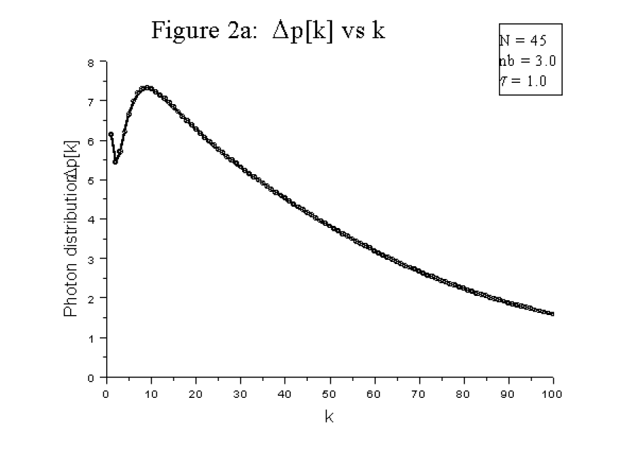
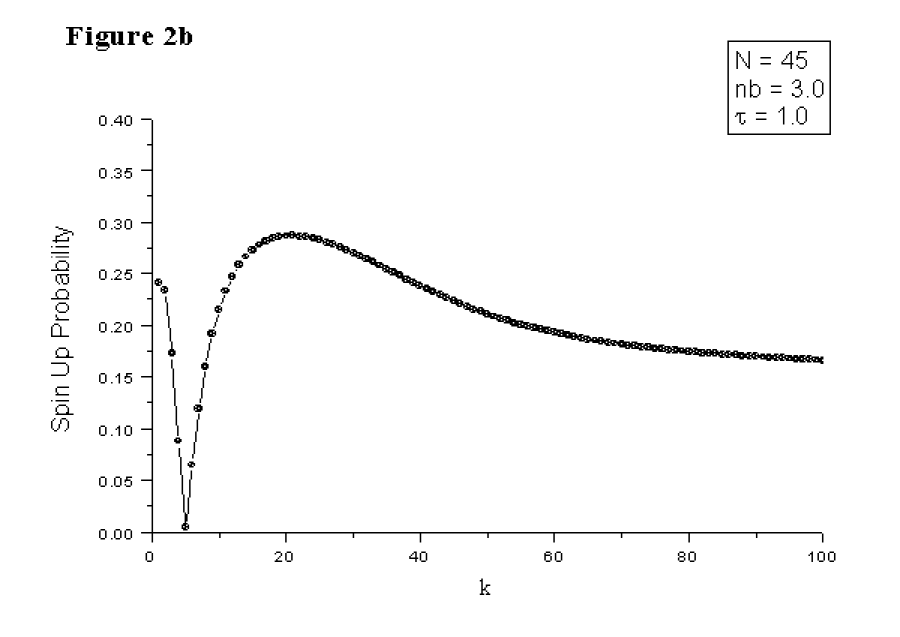
Figure 2: Variation of (a) $\Delta p(k)$ and (b) $\Delta P_{+}(k)$ with $k$

This test compares the probability that the $kth$ atom will emerge in the excited state to the same probability at equilibrium. It therefore has direct physical relevance. Figs. 2a) and 2b) plot $\Delta p(k)$ and $\Delta P_{+}(k)$ as functions of $k$ for $N=45$, $n_{b}=3.0$ and $\tau=1.0$. It is interesting that the system first moves towards equilibrium (very rapidly for $\Delta{\cal P}_{+}(k)$) and then moves away from equilibrium before it settles into its exponential approach to equilibrium. This feature appears to be fairly generic for large $N$.

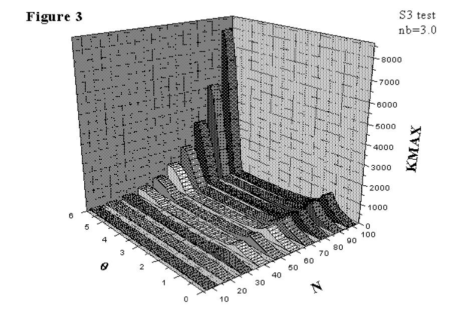
Figure 3: Variation of $k_{max}$ with $\theta$ and $N$ for fixed $n_{b}=3$ for the two tests described in the text.

In order to do a systematic analysis of the convergence rate as a function of the physical parameters, we define $k_{max}$ as the number of atoms it takes for $\Delta p(k)$ to get to some critical value, $\Delta_{crit}$, or less. For small enough $\Delta_{crit}$, $k_{max}$ should be large, in which case the convergence will be determined by the next to leading eigenvalue of $S$. Fig. 3 plots $k_{max}$ as obtained from the two tests as functions of $\theta$ and $N$ for $n_{b}=3$, with the condition $\Delta_{crit}=0.005$. Clearly the resulting values of $k_{max}$ are large enough to be in the region of asymptotic convergence and the phase structure is the same as that predicted analytically using the eigenvalues of $S$. This result confirms the validity of our numerical method.

We now use the numerical experiments to investigate a different but related property of convergence. In particular, we look at how $k_{max}$ is affected by a change in $n_{b}$ and $N$ for fixed interaction time. As shown in Fig. 4, as $n_{b}$ gets large, the convergence is uniformly rapid for all $N$, whereas for low $n_{b}$ (i.e. low temperatures) there are critical values of $N$ for which convergence slows suddenly. These are presumably the same transitions as in Fig. 1 but seen from a different view. In particular, lines of fixed $n_{b}$ and $g\tau$ correspond to a section of Fig. 1 with $\theta=g\tau\sqrt{N}.$ Fig. 5 shows this structure for fixed $n_{b}$ and $g\tau$. As shown in Fig. 6, these “steps” in the convergence coincide (at least approximately) with values of the parameters in which the correlation length, as determined by the leading eigenvalue, increases. Fig. 6 plots the correlation lengths for $n_{b}=1$ for the first four leading eigenvalues. It is interesting that the “steps” correspond to points where the eigenvalues appear to cross. However, the eigenvalues are not degenerate [3], so the curves do not actually intersect. In Fig. 7 the equilibrium photon distributions are plotted for $nb=1$ as a function of $N$. It shows clearly that the “crossing” of the eigenvalues is related to a discrete shift in the peak of the equilibrium photon distribution. The crossings, and the associated transitions in the convergence rate illustrated in Fig. 5, occur when the photon distribution is in the process of shifting, i.e. where there are two peaks.

5 Conclusions

We have presented a systematic analysis of the discrete master equation describing the approach to equilibrium of the micromaser in the presence of thermal dissipation. As expected, the long time behaviour is determined by the leading eigenvalues of the discrete transformation matrix. Interestingly, the eigenvalues of the matrix, evaluated numerically, become at some places nearly degenerate, and the phase structure of the micromaser occurs at or near where the eigenvalues come close to crossing. Our analytic results confirm general features that emerge from the continuous master equation in [3]. We also have examined the approach to equilibrium of the micromaser both at short and long times using numerically methods. Our numerical results are consistent with the behaviour expected from the leading eigenvalues of both the discrete and continuous transformation matrices. However, our results also show some interesting feature for short times; in particular, the system in general first approaches equilibrium relatively rapidly, then moves away from equilibrium, and then finally settles into its exponential approach to equilibrium. This behaviour appears to be fairly generic for large values of $N$, but more analysis is required to determine the source and relevance of these short time features. Moreover we have, in the numerical experiments, kept the transit time fixed. In future work we hope to examine how varying $g\tau$ affects the above mentioned features.

Acknowledgements

This work was supported in part by the Natural Sciences and Engineering Research Council of Canada, and by Career Focus, Manitoba.

Appendix: The Relationship Between the Continuous and Discrete Cases

We expect differences in the dynamical behaviour in the discrete and continuous formalisms, but there should exist a limit in which the two formalisms coincide. We look at the discrete formalism in the large flux limit. We take $k=Rt$ to be large, which means that $t\gg 1/T$, or that the total time over which the system is observed is much greater than the time between individual atoms.

To take the large flux limit of the discrete master equation, we follow the derivation of Eq.(3). The discrete master equation has the form Eq.(32),

$$p^{k+1}=Sp^{k}$$ (83)

We write,

$$p^{k+1}-p^{k} = (S-1)p^{k}$$

$$(p^{k+1}-p^{k}) = T[T^{-1}(S-1)T]T^{-1}p^{k}$$

$$p_{b}^{k+1}-p_{b}^{k} = T_{bn}[(\kappa^{(n)}-1)\delta_{nm}](T^{-1}p^{k})_{ma}$$ (84)

which can be written in differential form as,

$$d\,p=-(1-S)pd\,k$$ (85)

Since $k=Rt$ we can write $d\,k=Rd\,t$ and compare Eq.(35) and Eq.(85):

$$-\gamma L = -(1-S)R$$

$$L = N(1-S);\,\,\,\,\,\,R/\gamma=N$$ (86)

Using Eq.(32) and Eq.(35) we find,

$$L_{C}-N(M-1)={\tilde{N}}-{\tilde{N}}\frac{1}{1+L_{C}/{\tilde{N}}}M$$ (87)

We study the behaviour of the next to leading eigenvectors, since the corresponding eigenvalues control the behaviour of the approach to equilibrium. We have,

$$(L_{C}-N(M-1))p^{(2)}=\lambda^{(2)}p^{(2)}$$ (88)

and

$$S\tilde{p}^{(2)} = \kappa^{(2)}\tilde{p}^{(2)}$$

$$\rightarrow\frac{1}{1+L_{C}/\tilde{N}}M\tilde{p}^{(2)} = \kappa^{(2)}\tilde{p}^{(2)}$$

$$\rightarrow(L_{C}-\frac{\tilde{N}(m-1)}{\kappa^{(2)}})\tilde{p}^{(2)} = \tilde{N}[\frac{1}{\kappa^{(2)}}-1]\tilde{p}^{(2)}$$ (89)

Comparing Eq.(88) and Eq.(89) we have,

$$N=\tilde{N}/\kappa^{(2)};\,\,\,\,\,\,\,\,\,\,\,\lambda^{(2)}=\tilde{N}[\frac{1}{\kappa^{(2)}}-1]$$ (90)

Solving this set of equations we have,

$$\kappa^{(2)}=1-\frac{\lambda^{(2)}}{N}$$

$${\rm ln}\kappa^{(2)}={\rm ln}(1-\frac{\lambda^{(2)}}{N})\sim-\frac{\lambda^{(2)}}{N}$$

$$-R{\rm ln}\kappa^{(2)}\sim\frac{R}{N}\lambda^{(2)}=\gamma\lambda^{(2)}$$ (91)

where we have taken $N$ large, or $1/\gamma\gg T$, which means that the typical photon decay time is much greater than the typical time between atoms.

Figures

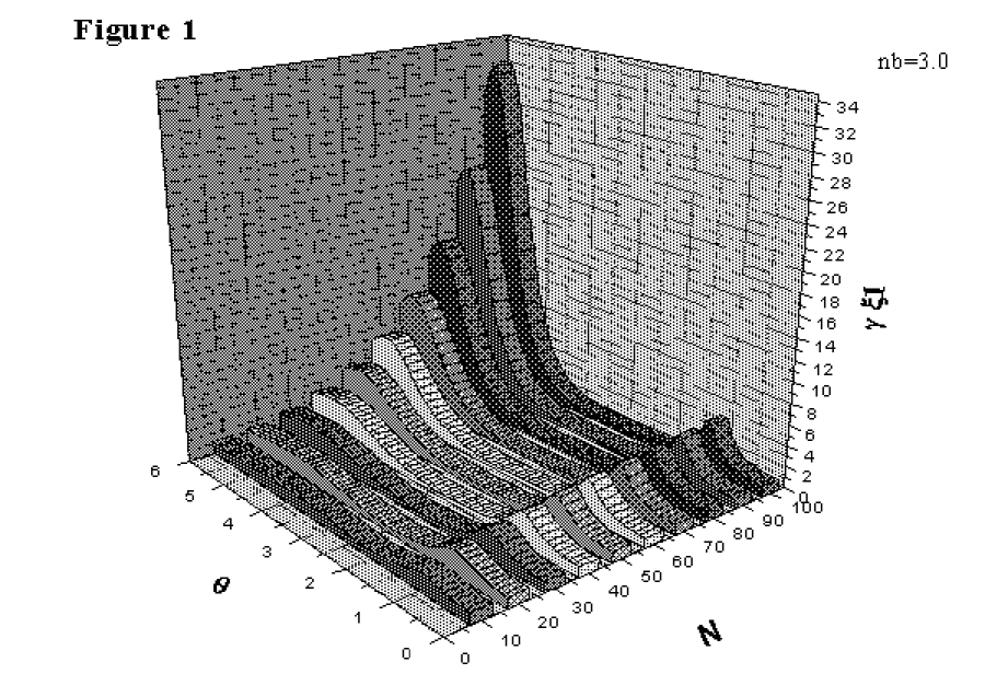
Figure 1: Variation of ccorrelation length with pumping rate and interaction time for fixed $n_{b}=3$

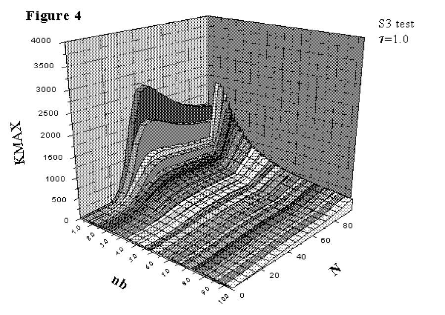
Figure 4: Variation of $k_{max}$ with $n_{b}$ and $N$ for fixed interaction time.

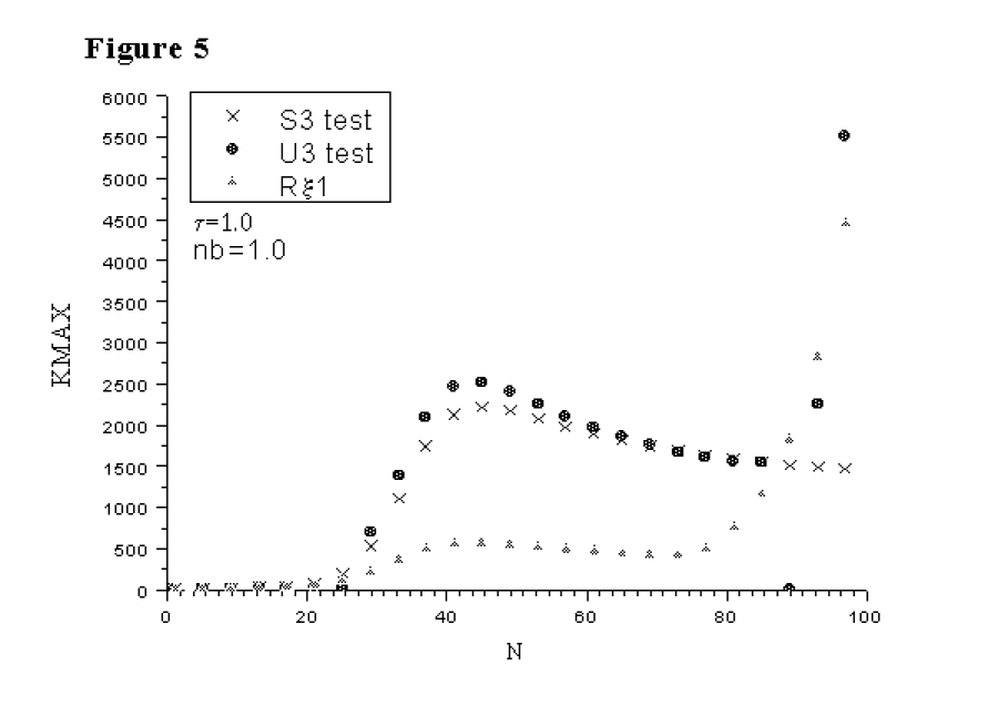
Figure 5: Variation of $k_{max}$ with $N$ for fixed $n_{b}$ and $g\tau$.

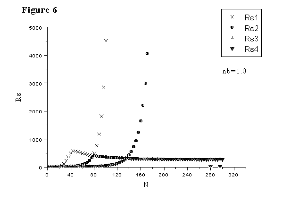
Figure 6: Variation of correlation lengths with $N$ for $n_{b}=1$ for the first four leading eignevalues.

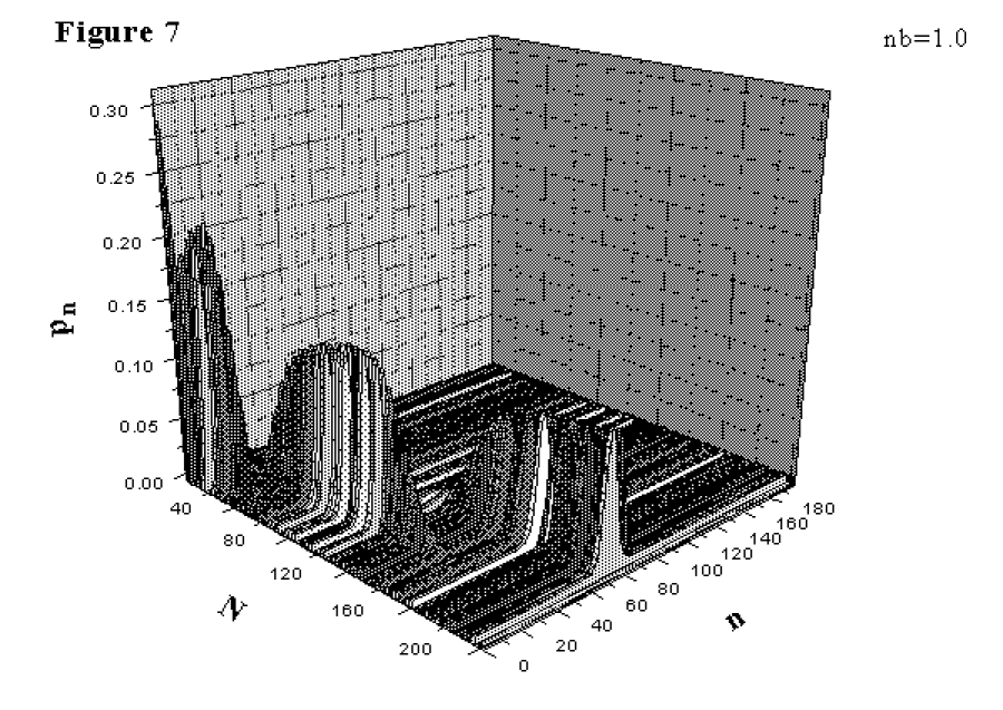
Figure 7: Plots of the equilibrium photon distributions for $n_{b}=1$ as a function of $N$

References

- [1] P. Goy, J.M. Raimond, M. Gross and S. Haroche, Phys. Rev. Lett. 50, 1903 (1983); D. Meschede, H. Walther and G. Muller, Phys. Rev. Lett. 54, 551 (1985). For a reviews see, for example, D. Meschede, Phys. Rep. 211, 201 (1992) and H. Walther, PHys. Rep. 219 263 (1992).
- [2] E.T. Jaynes and F.W. Cummings, Proc. IEEE 51, 89 (1963).
- [3] P. Elmfors, B. Lautrup an B. Skagerstam, atom-ph/9601004v2 (1996).
- [4] G. Rempe and H. Walther, Phys. Rev. Lett. 58, 353 (1987).