1

STRUCTURE OF PHYSICAL SPACE

AND NATURE OF ELECTROMAGNETIC FIELD

Yuri A. Baurov

Central Research Institute of Machine Building

Pionerskaya, 4

141070, Korolyov, Moscow Region, Russia

In the article, on the basis of the author’s model of formation of the observable physical space $R_{3}$ in the process of dynamics of special discrete one-dimensional vectorial objects, byuons, while minimizing their potential energy of interaction in the one-dimensional space $R_{1}$ formed by them, and based on the Weyl’s geometrical model of the electromagnetic field, the nature of this field consisting in a suitable variation of byuon interaction periods in the space $R_{1}$ , is shown.
PACS numbers: 11.23

1 Introduction

A wealth of works, beginning from antiquity (Aristoteles^?, ”The Principia” by Euclides, Democritus) and ending with authors of 20th century, are dedicated to the structure of space and time, to the physical sense of these fundamental concepts, and their properties. For brevity sake, we will not give an extensive bibliography on the subject but advise the reader to acquaint himself only with two monographs ^?,?, in the first of which a physical and philosophical comprehension of hundreds of works on this problem is presented, and in the second, an ingenious work of a known russian physicist D.I.Blokhintsev, difficulties encountered in describing the world of elementary particles when creating a modern space theory, are shown. In all existing works on quantum field theory and physics of elementary particles, the space in which elementary processes occur, as a rule, is given one way or another. Further the action $S_{1}$ is written in the given space in terms of the Lagrangian function density for the fields and objects considered, and equations of motion are obtained for the system considered in the given space from the least action principle. Yet we will follow another way and try to build physical space and major properties of elementary objects in this space from dynamics of a finite set of special discrete objects (so called byuons) ^?,?. Note that the development of physical comprehension of elementary processes on the base of modern superstring models ^?-?, unfortunately, also gives no evidences for how structured is the observed space itself which is obtained, according to one of the models, by means of compactification of six dimensions in a ten-dimensional space. New theoretical approaches found in construction of physical space have given the chance to look in a new way also at the most studied object of the classic and quantum field theory, the electromagnetic field. In the present paper we will not touch upon many problems widely covered in the literature and concerned with the photon and electromagnetic field: whether the photon has a rest mass (Proc’s equation), whether or not it possesses a longitudinal component of field, being artificially removed by the Lorentz’s condition ^?, etc. We try only to explain the origin of the Maxwell’s equations as a peculiar change in the structure of physical space due to dynamics of byuons. Chronologically, the author has arrived to the theory of byuons when investigating a system of spinor and boson fields interacting with the electromagnetic field ^?-?.As a generalized coordinate in this system, the velocity of propagation of interactions $c=c(x,t)$ was taken where $x$ is the coordinate of a certain one-dimensional compact space $M_{1}$, $t$ is time, and the electric charge $e$ of the fields is assumed to be some implicit function of $c(x,t)$, i.e. $e=e[c(x,t)]$. Thus the author anticipated the local violation of gauge invariance and Lorentz’s group extended on translation (Poincaret’s group) in order to gain an insight into the process of physical space formation.

2 Fundamental Theoretical Concepts of Physical Space Origin.

In Ref. ^?,?, the conception of formation of the observed physical space $R_{3}$ from a finite set of byuons is given. The byuons ${\bf\Phi}(i)$ are one-dimensional vectors and have the form:

$${\bf\Phi}(i)={\bf A_{g}}x(i),$$

where $x(i)$ is the ”length” of the byuon, a real (positive, or negative) value depending on the index $i=0,1,2,...,k...$, a quantum number of ${\bf\Phi}(i)$; under $x(i)$ a certain time charge of the byuon may be meant (with $x(i)$ in centimeters). The vector ${\bf A}_{g}$ represents the cosmological vectorial potential, a new basic vectorial constant ^?,?,?,?. It takes only two values:

$${\bf A}_{g}=\left\{A_{g}\atop-\sqrt{-1}A_{g}\right\},$$

where $A_{g}$ is the modulus of the cosmological vectorial potential ($A_{g}\approx 1.95\times 10^{11}$ CGSE units). According to the theory ^?,?, the value $A_{g}$ is the limiting one. In reality, there exists in nature, in the vicinity of the Earth, a certain summary potential, i.e. the vectorial potential fields from the Sun ($A_{\odot}\approx 10^{8}$ CGSE units), the Galaxy ($\sim 10^{11}$ CGSE units), and the Metagalaxy ($>10^{11}$ CGSE units) are superimposed on the constant $A_{g}$ resulting probably in some turning of ${\bf A}_{\Sigma}$ relative to the vector ${\bf A}_{g}$ in the space $R_{3}$ and in a decrease of it.

Hence in the theory of physical space (vacuum) which the present article leans upon, the field of the vectorial potential introduced even by Maxwell gains a fundamental character. As is known, this field was believed as an abstraction. All the existing theories are usually gauge invariant. For example, in classical and quantum electrodynamics, the vectorial potential is defined with an accuracy of an arbitrary function gradient, and the scalar one is with that of time derivative of the same function, and one takes only the fields of derivatives of these potentials, i. e. magnetic flux density and electric field strength, as real.

ln Refs.^?-?,local violation of the gauge invariance and Poincaret’s group was supposed, and the elementary particle charge and quantum number formation processes were investigated in some set, therefore the potentials gained an unambiguous physical meaning there. In the present paper, this is a finite set of byuons.

The works by D.Bohm and Ya.Aharonov ^? discussing the special meaning of potentials in quantum mechanics are the most close to the approach under consideration, they are confirmed by numerous experiments ^?.

For understanding the byuon dynamics, present an extract from the author’s materials of investigations on metrics in the one-dimensional compact space $M_{I}$ ^?.

Let us assume that the velocity $c$ in the space $M_{I}(x,t)$ is a function of $x$ and $t$, i.e. $c=c(x,t)$. Then the metrics of such a manifold may be represented as

$$d[c(x,t)t]^{2}-dx^{2}=0.$$

Rewrite Eq. (1) in the form

$$\{d[c(x,t)t]-dx\}\{d[c(x,t)t]+dx\}=0.$$

Removing brackets in Eq.(2) and dividing it by $dt$ yield two equations

$$t\frac{\partial c}{\partial t}+c+t\frac{\partial c}{\partial x}\frac{dx}{dt}-\frac{dx}{dt}=0,$$

$$t\frac{\partial c}{\partial t}+c+t\frac{\partial c}{\partial x}\frac{dx}{dt}+\frac{dx}{dt}=0.$$

At limiting points of the compact space $M_{I}$ the differentials $dx$ and $dt$ are not independent, therefore we may assume $\frac{dx}{dt}=c$. Then we have from Eq.(3)

$$(3.1)\Rightarrow\frac{\partial c}{\partial t}+\frac{\partial c}{\partial x}c=0,$$

$$(3.2)\Rightarrow t\frac{\partial c}{\partial t}+t\frac{\partial c}{\partial x}c+2c=0.$$

Eq.(4) with boundary conditions $t=t_{o},x=x_{o}$ has a solution $c(x,t)=const=c_{o}$, which is in accord with a postulate of special theory of relativity.

Seek a solution of Eq.(5) with the same boundary conditions as for Eq.(4). The system of characteristic equations may be written as ^?:

$$\frac{dc}{dt}=\frac{\partial c}{\partial t}+c\frac{\partial c}{\partial x},$$

$$\frac{dx}{dt}=c,$$

$$\frac{d(\frac{\partial c}{\partial x})}{dt}=-\frac{\partial c}{\partial x}\left(\frac{\partial c}{\partial x}+\frac{2}{t}\right),$$

$$\frac{d(\frac{\partial c}{\partial t})}{dt}=-\left[\frac{\partial c}{\partial t}\left(\frac{\partial c}{\partial x}+\frac{2}{t}\right)-\frac{2c}{t^{2}}\right].$$

Solving Eq. (8), we find

$$c(x,t)=\frac{x}{t(t/t^{*}-1)}+f(t).$$

Here $t^{*}$ is constant of integration, $f(t)$ an arbitrary function of $t$. Setting $f(t)=0$ in Eq.(10) gives

$$c(x,t)=\frac{x}{t(t/t^{*}-1)}.$$

The function $c(x,t)$ satisfies (5) and at a fixed $x_{0}$ has the form shown in Fig. 1. As is seen, $c(x,t)$ has discontinuities at $t=t^{*}$ and $t=0$. Since a signal from point $x_{1}$ to point $x_{2}$ in $M_{I}$ cannot be transmitted instantaneously (with the infinite speed), we assume that only the limiting values $c=\pm c_{0}$ can be realized in nature. One may come to this conclusion when considering non-classical variation calculus, too. It is known from Ref. ^? that if restrictions are imposed on a variable function minimizing a functional (in our case, $c(x,t)$ may be thought of as imposed on by inequalities $-c_{0}\leq c(x,t)\leq c_{o}$ due to physical vacuum properties), then, from the viewpoint of minimum functional, only boundary values of the function being varied should be optimum.

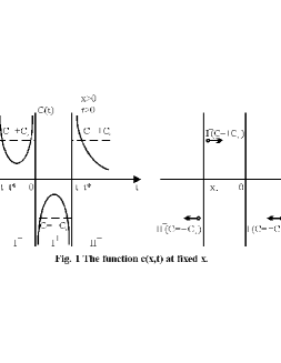
Figure 1: The function $c(x,t)$ at fixed x.

The byuons may be in four vacuum states (VS) $II^{+},I^{+},II^{-},I^{-},$ in which they discretely change the value ot $x(i)$: the state $II^{+}$ discretely increases ($c=c_{0}=\tilde{x}_{0}/\tau_{0}$, where $\tilde{x}_{0}$ - quantum of space ($\approx 10^{-33}$cm), $\tau_{0}$ - quantum of time ($\approx 10^{-43}c$)) and $I^{+}$ decreases $x(i)>0$ ($c=-c_{o}=-\tilde{x}_{0}/\tau_{0}$); the states $II^{-}$ and $I^{-}$ discretely increase or decrease the modulus of $x(i)<0$, respectively ($II^{-}$ corresponds to $c=-c_{0}$, $I^{-}$ corresponds to $c=c_{0}$). The sequence of discrete changes of $x(i)$ value is defined as a proper discrete time of the byuon. The byuon vacuum states originate randomly ^?,?.

In Refs. ^?,?, the following hypothesis has been put forward: It is suggested that the space $R_{3}$ observed is built up as a result of minimizing the potential energy of byuon interactions in the one-dimensional space $R_{1}$ formed by them. More precisely, the space $R_{3}$ is fixed by us as a result of dynamics arisen of byuons. The dynamic processes and, as a consequence, wave properties of elementary particles appear therewith in the space $R_{3}$ for objects with the residual positive potential energy of byuon interaction (objects observed). Let us briefly list the results obtained earlier when investigating the present model of physical vacuum (see Appendix):

1. The existence of a new long-range interaction in nature, arising when acting on physical vacuum by the vectorial potential of high-current systems, has been predicted ^?,?.

2. All the existing interactions (strong, weak, electromagnetic and gravitational ones) along with the new interaction predicted have been qualitatively explained in the unified context of changing in three periods of byuon interactions with characteristic scales - $x_{0}=\tilde{x}_{0}k\approx 10^{-17}$cm, $ct^{*}=\tilde{x}_{0}kN\approx 10^{-13}$cm, and $\tilde{x}_{0}kNP\approx 10^{28}$cm, determined from the minimum potential energy of byuon interaction ^?,?.

3. Masses of leptons, basic barions and mesons have been found ^?,?.

4. The constants of weak interaction (vectorial and axial ones) and of strong interaction have been calculated ^?,?.

5. The origin of the galactic and intergalactic magnetic fields has been explained as a result of existence of an insignificant ($\approx 10^{-15}$) asymmetry in the formation process of $R_{3}$ from the one-dimensional space of byuons ^?,?.

6. The matter density observed in the Universe ($\approx 10^{-29}g/cm^{3}$) has been computated ^?,?.

7. The origin of the relic radiation has been explained on the basis of unified mechanism of the space $R_{3}$ formation from one-dimensional space $R_{1}$ of byuons ^?,?, etc.

Let us explain item 1 briefly. It is shown in Ref. ^? that masses of all elementary particles are proportional to the modulus of ${\bf A}_{g}$ (see Appendix). If now we direct the vectorial potential of a magnetic system in some space region towards the vector ${\bf A}_{g}$ then any material body will be forced out of the region where $|{\bf A}_{\Sigma}|<|{\bf A}_{g}|$ . The new force is nonlocal, nonlinear, and represented by a complex series in $\Delta A$, a difference in changes of $|{\bf A}_{\Sigma}|$ due to the potential of a current at location points of a sensor and a test body ^?,?. This force is directed mainly by the direction of the vector ${\bf A}_{g}$, but as the latest experiments have shown, there is also an isotropic component of the new force in natures, which component acts omnidirectionally from the space of the maximum decrease in $|{\bf A}_{\Sigma}|$. Corresponding to it are probably the even terms in a series representing the new force ^?,?.

One of the important predictions of the theory is revealing a new information channel in the Universe which is associated with the existence of a minimum object with positive potential energy, so called object $4b$, arising in the minimum four-contact interaction of byuons in the vacuum states $II^{+},I^{+},II^{-},I^{-}$. In four-contact byuon interaction, a minimum action equal to $h$ (Planck’s constant) occurs, and the spin of the object appears. Hence the greater part of the potential energy of byuon interaction is transformed into spin of the object $4b$. The residual (after minimization) potential energy of the object $4b$ is equal to $\approx 33eV$. It is identified with the rest mass of this object in the space $R_{1}$. In agreement with Refs. ^?,?, the indicated minimum object $4b$ has, according to Heisenberg uncertainty relation, the uncertainty in coordinate $\Delta x\approx 10^{28}$cm in $R_{3}$. The total energy of these objects determines near $98\%$ energy of the Universe as well as its matter density observed. In Refs. ^?,? it is shown that the existence of the $4b$-objects interpreted by the author as pairs of electron-type neutrino and electron-type antineutrino ($\nu_{e}\Leftrightarrow\tilde{\nu}_{e}$), causes a finiteness of the velocity of propagation of interaction c being an infinite quantity at $t=0$ and $t=t^{*}$ according to Eq. (11).

3 On The Nature Of The Electromagnetic Field.

Within the limits of an article it is difficult to unravel the problem as a whole, i.e. to develop a physical and mathematical model of the phenomenon. Therefore we dwell basically on a new physical model of the electromagnetic field resulting from the above presented model of physical space. But, as is known, the new is very often contained in the forgotten old if that is looked at in a new way.

Consider the Weyl’s geometrical model of the electromagnetic field ^?. Historically, the Weyl’s geometry was proposed for explaining by curvature of space not only the long-range gravitational field as in the theory of Einstein but another long-range field, the electromagnetic field, too.

Gravity is well explained by the Einstein’s theory in terms of space curvature. This suggests that the electromagnetic field also can be attributed to a certain space property instead of considering this field as simply ”immersed” in space. Thus, some more general space than the Riemannean space underlying the Einstein’s theory, had to be proposed to describe the existence of either gravitational or electromagnetic forces and to unify the long-range interactions.

The curvature of space required by the Einstein’s theory can be represented in terms of parallel displacement of a vector moving along a closed contour, which leads to the effect that the final direction of the vector will not be the same as the former. The Weyl’s generalization was in assuming that the final vector has not only a different direction but a different length, too (and this is the most important thing). In the Weyl’s geometry, there is no absolute procedure of comparing elements of length at two different points if these are not infinitely close to each other.

The comparison may be made only relative to a line segment connecting the two points, and different ways will give different results as to ratio of the two elements of length. In order to have mathematical theory of lengths one must arbitrarily establish a length standard at each point and then relate any length at anyone point to the local standard for this point. Then we will have a fixed value of the vector length at any point but this value varies with the local standard of length.

Let’s consider a vector of length $l$ positioned at a point with coordinates $x^{\mu}(\mu=1,2,3,4)$. Assume that this vector is transferred to the point $x^{\mu}+\delta x^{\mu}$. The change in its length $\delta l$ will be proportional to $l$ and $\delta x^{\mu}$ so that $\delta l=lk_{\mu}\delta x^{\mu}$ where $k_{\mu}$ is additional parameters of the field appearing in the theory together with the Einsteinean $g_{\mu\nu}$ and being equally fundamental.

Assume that the length standards have been changed so that lengths are multiplied by a coefficient $\lambda(x)$. Then $l$ goes into $l^{\prime}=l\lambda(x)$ and $l+\delta l$ does into

$$l^{\prime}+\delta l^{\prime}=(l+\delta l)\lambda(x+\delta x)=(l+\delta l)\lambda(x)+l\frac{\partial\lambda}{\partial x^{\mu}}\delta x^{\mu}.$$

Hence

$$\delta l^{\prime}=\lambda\delta l+l\frac{\partial\lambda}{\partial x^{\mu}}\delta x^{\mu}=\lambda l(k_{\mu}+\frac{\partial\lg\lambda}{\partial x^{\mu}})\delta x^{\mu}.$$

Thus, $\delta l^{\prime}=l^{\prime}k^{\prime}_{\mu}\delta x^{\mu}$ where

$$k^{\prime}_{\mu}=k_{\mu}+\frac{\partial\lg\lambda}{\partial x^{\mu}}$$

If our vector is transferred by parallel displacement along a closed contour, a change in its length will be $\delta l=l\Omega_{\mu\nu}\delta S^{\mu\nu}$ where

$$\Omega_{\mu\nu}=\frac{\partial k_{\mu}}{\partial x^{\nu}}-\frac{\partial k_{\nu}}{\partial x^{\nu}},$$

and $\delta S^{\mu\nu}$ notes an element of area limited by a small contour.

Let us show that the new field characteristic $k_{\mu}$ appearing in the Weyl’s theory have the meaning of electromagnetic potentials. As is known ^?,?, the antisymmetric tensor $F_{\mu\nu}$ of the electromagnetic field has the form $F_{\mu\nu}=\partial_{\mu}A_{\nu}-\partial_{\nu}A_{\mu}$ where $A_{\mu}$ and $A_{\nu}$ are components of the real covariant four-vectorial electromagnetic potential $A_{\alpha}(\alpha=0,1,2,3)$. Comparing the $\Omega_{\mu\nu}$ and $F_{\mu\nu}$ tensors we see that, indeed, the additional parameters characterizing proportionality of change in length of the vector $l$ while going from the point $x^{\mu}$ to the point $x^{\mu}+\delta x^{\mu}$, have the meaning of electromagnetic potentials. They go through the transformations (12) corresponding not to a change in geometry but only to a change in choosing artificial length standards. The derivatives $\Omega_{\mu\nu}$ have a geometrical meaning without regard to standards of length and correspond to physically significant parameters, electric and magnetic fields. Thus, the geometry of Weyl assures just what is necessary for describing the gravitational and electromagnetic fields in terms of geometry.

Hence when assuming a mathematical algorithm of transition of events from $R_{1}$ to $R_{3}$ as having been found, the electromagnetic and gravitational interaction of objects can be assured by changing period of byuon interactions $k,N$ and scale lengths $x_{0}$ and $ct^{*}$, respectively. The electromagnetic field is caused therewith by changing $|{\bf A}_{\Sigma}|$ due to some scalar $A_{0}$, and magnetic field is due to a vectorial potential ${\bf A}$ but with the complete return of the vector ${\bf A}$ to the initial point of the $R_{3}$ - space while tracing some closed contour l (i.e. in the absence of spacial anisotropy). Note once more that the electromagnetic constant of interaction (fine structure constant) $e^{2}/hc_{0}$ will be constant in all reference systems (see Appendix).

Let’s now answer the question ”At the cost of which VSs of byuons is the electromagnetic field (i.e. variation of $l$ at the cost of $x_{0}$ and $ct^{*}$ variations) described ?” There can be two such variants of byuons VSs for describing the electromagnetic field (waves, photons). These are the pairs of byuons in VS $II^{+}I^{-}$ and pairs in VS $II^{-}I^{+}$. The later is explained by the fact that, for example, VSs $II^{+}$ and $I^{-}$ have, firstly, the same $c=c_{0}$, and secondly, they propagate in the same direction of the $R_{1}$-space (similarly for VS $II^{-}I^{+}$). Explain the former. If byuon VSs have the same $c$, then, in accordance with the ideology of charge formation ^?, the quantum transitions (correlation) between them cannot lead to formation of electric charge since to do this, the presence of VSs with opposite magnitudes of c is quite necessary for locking information within some local region of the space $R_{1}$ and hence $R_{3}$.

4 Conclusion.

Thus, it is qualitatively shown in the article that at the cost of varying periods of byuon interaction, it is possible to describe the electromagnetic field basing on the Weyl’s geometrical theory of this field.

Appendix A

In ^?,? by using an unordinary varying the action for the system of spinor and boson fields interacting with electromagnetic one, taking $c(x,t)$ as a generalized coordinate, considering $e=e[c(x,t)]$, the following formal results are obtained:

1. Expressions for $h$ and leptons are found:

$$h=\frac{(|{\bf A}|x_{0})^{2}}{c}\times\frac{x_{0}}{ct^{*}},$$

$$m_{e}=m_{\nu_{e}}\frac{ct^{*}}{x_{0}},\hskip 28.45274ptm_{\mu}=m_{\nu_{\mu}}\frac{ct^{*}}{2x_{0}},\hskip 28.45274ptm_{\tau}=m_{\nu_{\tau}}\frac{ct^{*}}{8x_{0}},$$

$$m_{\nu_{\mu}}c^{2}=|{\bf A}|A_{0}\frac{2x_{0}^{3}}{(ct^{*})^{2}},\hskip 28.45274ptm_{\nu_{\tau}}c^{2}=|{\bf A}|A_{0_{\tau}}\frac{24\times 8x_{0}^{3}}{(ct^{*})^{2}},$$

$$A_{0}e=\frac{1}{2}(|{\bf A}|x_{0})\times\left(\frac{x_{0}}{ct^{*}}\right)^{2}\times|{\bf A}|,\hskip 28.45274ptA_{0}=\frac{2\sqrt{3}e}{\sqrt{x_{0}ct^{*}}},\hskip 28.45274ptA_{0_{\tau}}=\frac{2\sqrt{3}e}{\sqrt{2x_{0}ct^{*}}}.$$

From these relationships three important conclusions follows:

$$|{\bf A}|x_{0}=\frac{(hc)^{3/2}}{4\sqrt{3}e^{2}}=const_{1},$$

$$\frac{x_{0}}{ct^{*}}=\left(\frac{4\sqrt{3}e^{2}}{hc}\right)^{2}=const_{2},$$

$$e^{2}=\frac{(|{\bf A}|x_{0})^{2}}{4\sqrt{3}}\times\left(\frac{x_{0}}{ct^{*}}\right)^{3/2}.$$

2. The expressions for the Planck’s constant $(A.1)$ and value of electric charge $(A.7)$ are invariant relative to variation of the parameters $|{\bf A}|$, $x_{0}$, $ct^{*}$ in the relationships $(A.5)$ and $(A.6)$. Hence, when varying, for example, $x_{0}$ and $ct^{*}$ so that the ratio $(A.6)$ is always equal to $const_{2}$, the expressions for $h$ $(A.1)$ and $e$ $(A.7)$ will remain unchanged. Similar is the situation with the parameters $|{\bf A}|$ and $x_{0}$ in $(A.5)$. Thus, we arrive to a conclusion that in nature there are possible a certain set of earlier unknown objects determined by the product ${\bf A}\times x_{0}$ which our world is based on, since its fundamental properties, particularly electromagnetic ones (the fine structure constant ${e^{2}}/{hc}$) determined by such constants as $h,e,c$, remain unchanged on this set.

3. Expressions for axial and vectorial constants of weak interactions, are deduced :

$$c_{A}=\frac{1}{2}e_{0}^{2}x_{0}ct^{*}\approx 1,4333\times 10^{-49}erg\cdot cm^{3},$$

$$c_{V}=2x_{0}^{3}\left(e_{0}|{\bf A}|+\frac{hc}{4x_{0}}\right)\approx 1,4336\times 10^{-49}erg\cdot cm^{3}.$$

4. Constant of strong interactions for proton: $g^{2}_{p}=\frac{1}{6}$, for $\pi^{0}$-meson: $g_{\pi^{0}}^{2}=\frac{4}{6}$ and expressions for masses of these particles, are obtained:

$$m_{p}c^{2} \approx \frac{\sqrt{hc}}{2}\left(\frac{4\sqrt{3}e^{2}}{hc}\right)^{3}\times\left\{1-\frac{1}{2}\sqrt{\frac{3x_{0}}{ct^{*}}}\right\}\times$$

$$\qquad\qquad\left[\sqrt{1+\frac{1}{6}\left(1-\frac{1}{2}\sqrt{\frac{3x_{0}}{ct^{*}}}\right)^{-2}}+1\right]\times|{\bf A}|\approx 924MeV,$$

$$m_{\pi_{0}}c^{2} \approx \frac{\sqrt{hc}}{2}\left(\frac{4\sqrt{3}e^{2}}{hc}\right)^{3}\times\left\{1-2\sqrt{\frac{3x_{0}}{ct^{*}}}\right\}\times$$

$$\qquad\qquad\left[\sqrt{1+\frac{1}{6}\left(1-2\sqrt{\frac{3x_{0}}{ct^{*}}}\right)^{-2}}-1\right]\times|{\bf A}|\approx 132MeV.$$

Also as it is shown in Ref. ^?, masses of all leptons are proportional to the modulus of ${\bf A}$, too:

$$m_{e}c^{2} = \frac{\sqrt{hc}}{2k}\left(\frac{hc}{4\sqrt{3}e^{2}}\right)^{3}\times|{\bf A}|,\,\,m_{\nu_{e}}c^{2}=\frac{\sqrt{hc}}{2k}\left(\frac{hc}{4\sqrt{3}e^{2}}\right)\times|{\bf A}|;$$

$$m_{\mu}c^{2} = 3^{1/4}\sqrt{hc}\left(\frac{4\sqrt{3}e^{2}}{hc}\right)^{3,5}\times|{\bf A}|,\,\,m_{\nu_{\mu}}c^{2}=2\times 3^{1/4}\sqrt{hc}\left(\frac{4\sqrt{3}e^{2}}{hc}\right)^{5,5}\times|{\bf A}|;$$

$$m_{\tau}c^{2} = 12\sqrt{2}\times 3^{1/4}\sqrt{hc}\left(\frac{4\sqrt{3}e^{2}}{hc}\right)^{3,5}\times|{\bf A}|,\,\,$$

$$\qquad\qquad\qquad m_{\nu_{\tau}}c^{2}=96\sqrt{2}\times 3^{1/4}\sqrt{hc}\left(\frac{4\sqrt{3}e^{2}}{hc}\right)^{5,5}\times|{\bf A}|.$$

5. The size of space quantum $\tilde{x}_{0}$ (without introducing the gravitation force), is found:

$$\tilde{x}_{0}=2\sqrt{3}\left(\frac{4\sqrt{3}e^{2}}{hc}\right)^{9}\times\frac{hc}{m_{e}c^{2}}\left(\frac{m_{e}}{m_{\mu}}\right)^{2}\approx 2,77986\times 10^{-33}cm.$$

6. The electric, barion, and lepton charges, as well as strangeness, are defined. Note that masses of all leptons, $p$ and $\pi^{0}$-mesons are expressed in terms of the single constant, modulus of a certain vectorial potential ${\bf A}$. Note once more that the size of space quantum is found without introducing gravitational force. Both conclusions are very important as showing that the nature of gravitation may be explained by way of developing physical views. With the use of a known fact of proportionality of space quantum to $\sqrt{\frac{Gh}{c^{3}}}$, where $G$ is the gravitational constant, one may show that

$$\frac{\sqrt{G}}{c^{2}}=\left(\frac{hc}{4\sqrt{3}e^{2}}\right)\times(0,6861k|{\bf A}|)^{-1}.$$

7. The value of magnetic flux density $B$ in $R_{3}$-space can be represented as $\frac{1}{16}\times\frac{|{\bf A_{g}}|\tilde{x}_{0}}{4\pi x_{0}^{2}}\times\frac{\tilde{x}_{0}}{x_{0}}$ where $\frac{\tilde{x}_{0}}{x_{0}}$ is sine of the angle between the byuon and the plane tangent to the sphere of radius $x_{0}$ at the point of byuon coming out. Estimations show that $B\approx 5\times 10^{-6}Gs$ ^?,?.

References

References

- [1] Aristoteles (v.3), Publishing House (PH) ”Mysl”, Moscow, 1987 (in Russian).
- [2] A.N.Vyaltsev, The discrete space-time, PH ”Nauka”, Moscow, 1965 (in Russian).
- [3] D.I.Blokhintsev, Space and time in the microworld, PH ”Nauka”, Moscow, 1982 (in Russian).
- [4] Yu.A.Baurov, in coll. work ”Plasma physics and some questions of the General Physics”, Central Institute of Machinery, Moscow region, Kaliningrad, 1990, pp.71,84 (in Russian).
- [5] Yu.A.Baurov, Fizicheskaya Mysl Rossii, 1, 18 (1994).
- [6] J.Scherk, J.H.Schwarz, Phys. Lett. B57, 463 (1975). E.Cremmer, J.Scherk, Mod. Phys., B103, 393 (1976), B108, 409 (1976).
- [7] J.H.Schwarz, Phys. Rept. 89, 223 (1982). M.B.Green, Surv. High Energy Phys. 3, 127 (1983).
- [8] M.Grin, J.Schwarz, and E.Vitten, Superstring Theory, in two volumes, PH ”Mir”, Moscow, 1990 (in Russian).
- [9] B.M.Barbashov, V.V.Nesterenko, Uspekhi Fizicheskikh Nauk (UFN) 150, 4, 489 (1986).
- [10] N.N.Bogolyubov and D.V.Shirkov, Introduction to the theory of quantized fields, PH ”Nauka”, Moscow, 1976 (in Russian).
- [11] Yu.A.Baurov, Yu.N.Babaev, and V.K. Ablekov, Dokl. Akad. Nauk (DAN) SSSR 259, 1080 (1981).
- [12] Yu.A.Baurov, Yu.N.Babaev, V.K. Ablekov, DAN, 262, 68 (1982).
- [13] Yu.A.Baurov, Yu.N.Babaev, V.K. Ablekov, DAN, 265, 1108 (1982).
- [14] Yu.N.Babaev, Yu.A.Baurov, Preprint P-0362 of Institute for Nuclear Research of Russian Academy of Sciences (INR RAS), Moscow, 1984 (in Russian).
- [15] Yu.N.Babaev, Yu.A.Baurov, Preprint P-0386 of INR RAS, Moscow, 1985 (in Russian).
- [16] Y.Aharonov, D.Bohm, Phys. Rev. 115, 485 (1959). Y.Aharonov, D.Bohm, Phys. Rev. 123, 1511 (1961). Y.Aharonov, D.Bohm, Phys. Rev. 125, 2192 (1962). Y.Aharonov, D.Bohm, Phys. Rev. 130, 1625 (1963).
- [17] M.Peshkin, A.Tonomura, The Aharonov-Bohm Effect., Springer-Verlag, Berlin, 1989, in Lecture Notes in Physics, p.154. G.N.Afanasjev, Fizika elementarnykh chastits i atomnogo yadra (EChAYa) 21, 1, 172 (1990); 23, 1264 (1992).
- [18] L.S.Pontryagin et al., Mathematical theory of optimum processes, PH ”Nauka”, Moscow, 1969 (in Russian).
- [19] Yu.A.Baurov, E.Yu.Klimenko, and S.I.Novikov, DAN 315, 1116 (1990). Yu.A.Baurov, E.Yu.Klimenko, S.I.Novikov, Phys. Lett. A162, 32 (1992). Yu.A.Baurov, P.M.Ryabov, DAN 326, 73 (1992).
- [20] Yu.A.Baurov, Phys. Lett. A181, 283 (1993).
- [21] H.Weyl, Raum, Zeit Material Vierte erweiterte Auflage, J.Springer, Berlin, 1921. H.Weyl, Space, Time, Matter, transl. from German, PH ”Yanus”, Moscow, 1996 (in Russian).
- [22] L.D.Landau, E.M.Lifshitz, Theory of the field, PH ”Nauka”, 1988 (in Russian).